1. Introduction
Precipitation is one of the most basic hydro-meteorological elements that has been a matter of concern for researchers, climatologists, and policymakers around the world [
1,
2,
3]. Urban areas have different influences on precipitation compared to the surrounding suburban and rural areas due to climatological differences [
4,
5]. This urban rain island (URI) [
6] effect has gained more attention in recent years due to an increasing number of urban areas with increased urbanization levels. Being a source of income opportunities and having improved living standards, cities are attracting more and more people. In 2018, the United Nations reported that about 55% of populations live in urban areas and the percentage is predicted to increase to 68% by 2050 [
7].
The percentage of impervious surfaces is higher in urban areas than in surrounding rural areas. Over time, several approaches have been undertaken by researchers to investigate the impact of urbanization on precipitation, such as using statistical analysis with a rain gauge, model simulations, or applying remote sensing-based data. Numerous studies have found significant evidence of urban influences on precipitation. While studying in La Porte, Indiana, ref [
8] noticed a sizeable increase in precipitation, moderate rain days, and hail days since 1925. There was about 31% more precipitation, 38% more thunderstorms, and 246% more hail days recorded in the La Porte station between 1951 and 1965 compared to the surrounding stations. Due to the proximity of La Porte to Chicago’s heavy industries (about 30 miles east), this study strongly suggested these increases were the effect of man-made modifications. There was about a 9 to 17% increase in warm seasonal rainfall reported by several researchers [
3,
8]. A detailed study during the 1970s, the ‘Metropolitan Meteorological Experiment’ (METROMEX), which was conducted in the USA, has shown increased precipitation during the summer months due to urban effects [
9]. Subsequently, ref [
10] mentioned that New York City was affected by summer daytime thunderstorms. In another study in Mexico City, ref [
11] observed a correlation between daytime UHI and intensified rain showers during the wet season (May to October). Upon further investigation, they noticed a positive correlation between the frequency of intense rainfall and the city’s size. Ref [
12] found significant anomalies in the annual precipitation and in the conditions during the warm season in and downwind of Houston, Texas. The urban heat island effect was found to be the primary reason for the precipitation anomalies. In a separate study, ref [
2] provided a detailed review of relevant studies on how the urban environment can affect precipitation. Ref [
13] also confirmed higher precipitation intensity downwind of Beijing, China.
In a recent study, Ref [
14] found a significant gap in the precipitation levels when comparing rapidly developed areas with slowly developing areas. While studying in Beijing, ref [
15] used hourly precipitation data from 43 rain gauges between 1980 and 2012. They also reported slightly greater amounts of precipitation in urban areas than in the surrounding suburbs. There was evidence of increased frequency and intensity of heavy precipitation due to urbanization in Shanghai [
16]. Ref [
17] found that the rain island effect in the different districts of Zhengzhou, China, became stronger with an increase in built-up areas. Ref [
18] suggested that the effects of urbanization on precipitation are not universal. For example, in coastal regions, urbanization would enhance sea breezes thereby positively influencing precipitation, whereas in inland areas, urbanization would lead to a warmer–drier climate.
So far, previous studies have tried to quantify and analyze precipitation on an aggregate scale such as for a city or for a particular region. However, until now, only a few studies have been conducted to see whether differences in precipitation are due to changes in the urbanization levels. Any particular urban area is not urbanized on the same level; some areas are highly urbanized, whereas others are less urbanized. This study is designed to assess responses to precipitation due to the urbanization level in Lagos, Nigeria. Another important thing to mention here is that this study will utilize the Google Earth Engine (GEE)—a cloud platform with terabytes of geospatial data—for all geospatial analyses. There are two main objectives of this innovative research—the first is to classify urbanization levels (non-urbanized, low-urbanized, mid-urbanized, and highly-urbanized) based on reliable urban characteristics, and the second is to assess the precipitation differences for each level.
Since Lagos is situated in Africa and is a rapidly growing urban hub, the study of this area will contribute greatly to urban climate research by exploring precipitation responses to urban development. A thorough understanding of this complex mechanism from a developing country such as Nigeria is needed, so this study could be a pioneer for similar future research activities.
2. Study Area
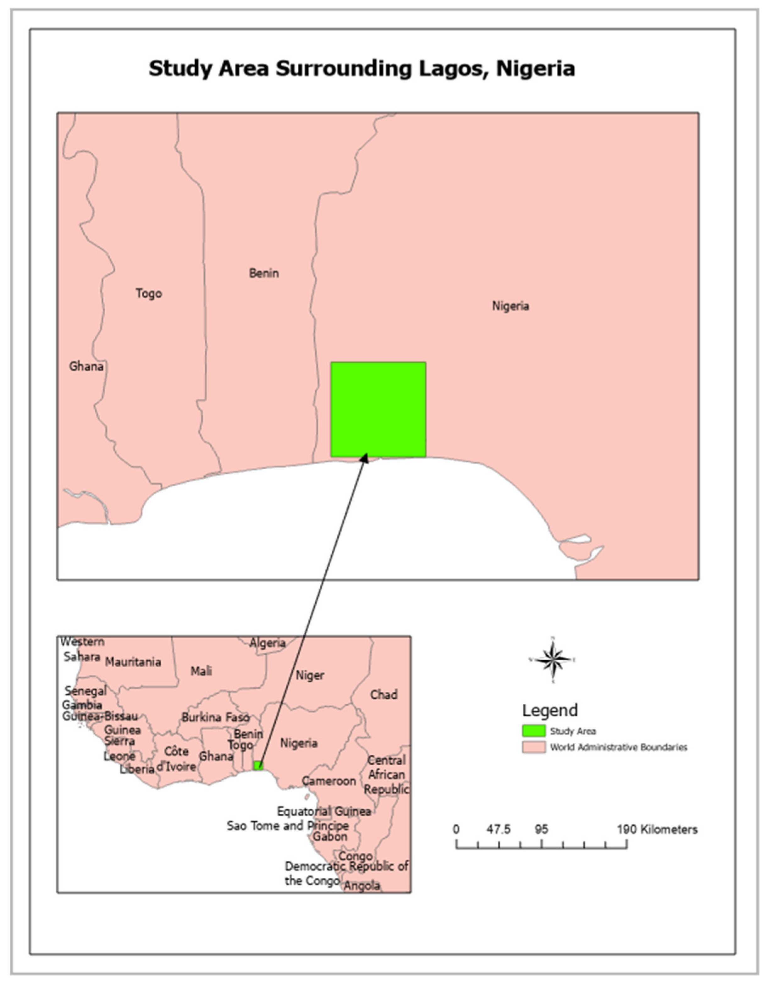
The primary focus of this study is Lagos, Nigeria, situated within latitudes 6°23′ N and 6°41′ N and longitudes 2°42′ E and 3°42′ E [
19]. Lagos is the chief port in Lagos State, Nigeria. It is a rapidly growing (both spatially and demographically) urban hub in the African continent. About 65% of Nigeria’s industries are based in Lagos, and they account for about 32% of Nigeria’s national gross domestic product (GDP) [
20]. From 1866 to 1911, Lagos’ total population grew from 25,000 to 73,766, covering a total area of 46.6 square kilometers. In 2006, this number reached 9,113,605 and the urban area expanded to 3345 square kilometers [
19]. As of 2021, Lagos’ population is about 14,862,111 with an urban coverage of 1171.28 square kilometers [
21].
There are four seasons observed in Lagos: late dry season, early wet season, late wet season, and early dry season, which correspond to January–March (JFM), April–June (AMJ), July–September (JAS), and October–December (OND) [
22], respectively.
As mentioned earlier, although the focus of this study is on Lagos City, due to analytical requirements, spatio-temporal dynamics, and long-term trend analysis, a larger rectangular region of about 9846.14 square kilometers around Lagos City has been considered (
Figure 1). This will help to explain spatial patterns over longer periods and how that pattern has evolved.
3. Data and Methods
The data requirements and methodology applied for this study will be discussed briefly in the following sub-sections.
3.1. Data
Several datasets are employed based on requirements for the different stages of analysis. For urban characterization, harmonized Defense Meteorological Satellite Program (DMSP) Visible Infrared Imaging Radiometer Suite (VIIRS) nighttime light and gridded population density data have been used, and the satellite precipitation data from the Climate Hazards Group Infrared Precipitation with Station (CHIRPS) have been used for the precipitation estimation.
3.1.1. Harmonized DMSP-VIIRS Nighttime Light
The U.S. Air Force DMSP has operated several satellite sensors since the 1970s that are capable of detecting visible and near-infrared emissions from cities and towns. The DMSP’s Operational Linescan System (OLS) has the unique capability of being able to capture low-light earth-imaging data during the night. The DMSP nighttime light values use digital numbers (DN) from 0–63 intensities. The data are available from 1992 to 2013. On the other hand, the VIIRS instruments aboard the joint NASA–NOAA Suomi National Polar-orbiting Partnership (Suomi NPP) and NOAA-20 satellites are providing global-scale visible and near-infrared (NIR) light during the night from 2012 to the present [
23]. The VIIRS day–night band (DNB) has higher spatial and radiometric resolution than the DMSP OLS, resulting in fewer over-glow effects and more city lights. The obvious differences in the nighttime light data collection as well as its attributes make it very difficult to deploy one singular dataset (either DMSP OLS or VIIRS DNB) for long-term monitoring. This requires integrating the two datasets and generating a harmonized product for continuous observation on a global scale. That requirement was duly noted by [
24] and they came up with a harmonized global-scale nighttime light dataset from 1992 to 2018.
3.1.2. Gridded Population Density
For population density, the Gridded Population of the World, Version 4 (GPW v4): Population Density, Revision 11 dataset will be used. This dataset consists of estimates of human population density (per square kilometer), which are consistent with national census and population registers, for the years 2000, 2005, 2010, 2015, and 2020 [
25]. To generate this gridded population density dataset, a proportional allocation gridding algorithm was applied by utilizing about 13.5 million national and sub-national administrative units. The data are freely available from the NASA Socioeconomic Data and Applications Center (SEDAC).
3.1.3. CHIRPS Precipitation Data
The CHIRPS is a quasi-global rainfall data set with over 35 years of observation and is created by the Climate Hazards Center at the UC Santa Barbara. The creation of the dataset was supported by drought monitoring efforts by the United States Agency for International Development Famine Early Warning Systems Network (USAID FEWS NET) [
26]. The dataset is built on previous approaches to ‘smart’ interpolation techniques and high resolution and contains long periods of records of precipitation estimates. The process of CHIRPS generation consists of three components: the Climate Hazards Group Precipitation climatology (CHPclim), the satellite-only Climate Hazards Group Infrared Precipitation (CHIRP), and the station-blending procedure.
3.2. Methods
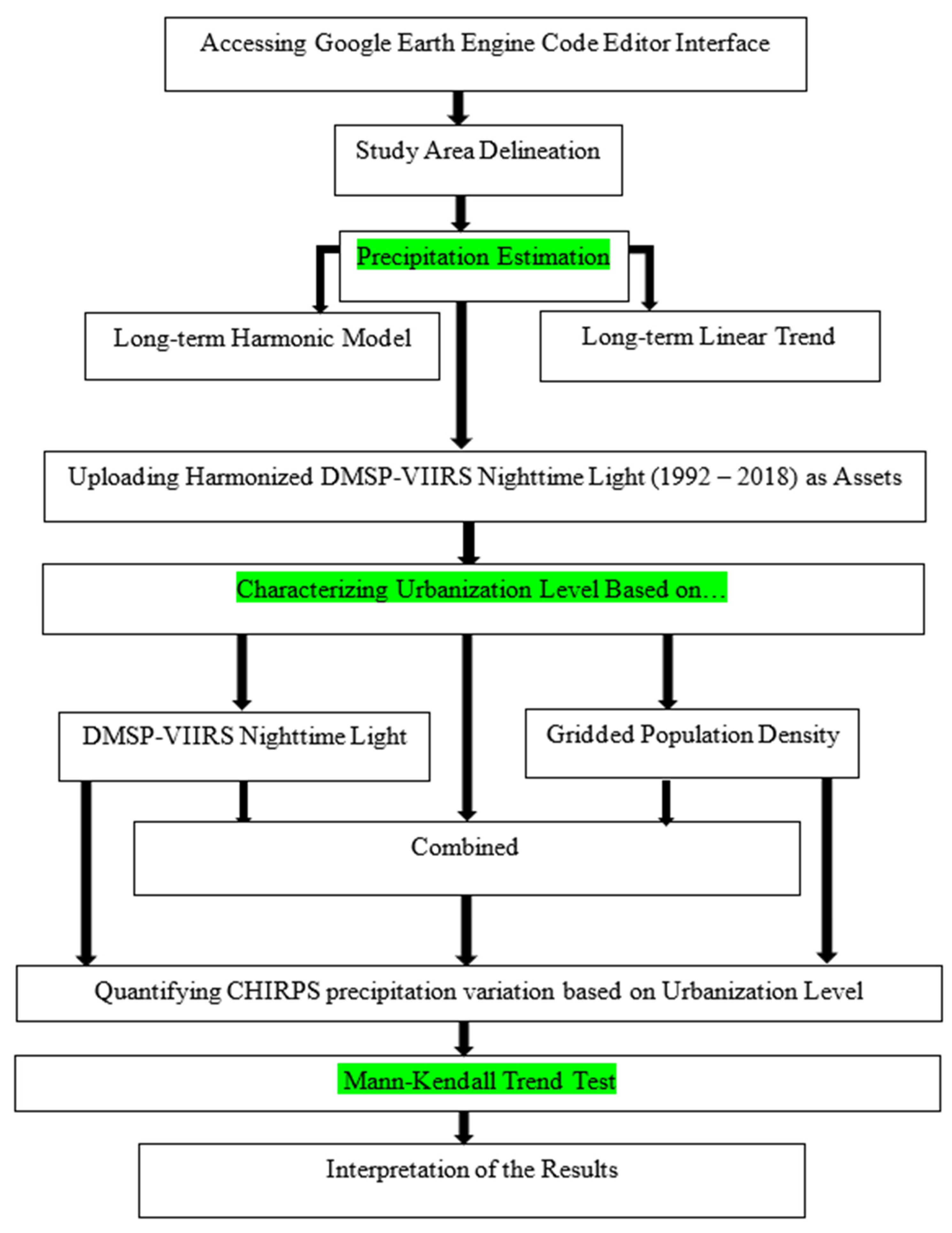
This study will utilize the above-mentioned data in different stages of analysis to meet the study objectives. The proposed method of this research will leverage the popular geospatial cloud computing platform [
27,
28,
29]—Google Earth Engine (GEE)—for performing all analyses. The entire work can be summarized in the following simplified workflow (
Figure 2).
The study is focused on two objectives—characterizing urban development intensity and estimating precipitation based on a different level of urban development intensity. In fact, the second objective is our main goal but working toward the first objective will help to achieve that goal. Initially, the study area will be considered at an aggregate level without being divided into any development zone. This will provide information about precipitation patterns for the whole study area. The next step would be to dive deep into the precipitation variations associated with urban development for the considered study period—from 1992 to 2018, or 27 years. First, urban characterization would be based on nighttime light, which has been one of the vital factors for explaining human activities, economic progress, and overall urban development. The results of this step will explain the precipitation patterns when urban development is characterized through the nighttime light passive indicator. Another influential criterion for explaining urbanization is the human population. In general, the more urbanized areas tend to have a higher population density than mid or less urbanized areas. So, the second stage of urban characterization would consider the population density in order to divide the study area into different development zones. The final step would be more advanced. Here, urbanization would be characterized not only based on a single criterion but through a combination of two factors. The idea is that this robust urban characterization would explain urbanization and its associated processes more clearly since it would consider human activities and human population density. Two urban areas with the same level of impervious surfaces but with different population densities would likely have different impacts. An urban area with a higher population density would have a higher impact than the other one with the comparatively less population density.
Precipitation estimations based on urbanization levels will initially require reliable variables that represent the different levels of urbanization/urban development as accurately as possible. Although both the DMSP and VIIRS nighttime light data are available through GEE, due to inconsistencies between the datasets (as discussed in the Data sub-section), a harmonized nighttime light dataset was uploaded toGEE as an ‘asset’. This ‘asset’ can be used when the other datasets are not readily available in GEE. There are three main steps (green colored in
Figure 2) in the workflow and they will be explained in detail in the following sub-sections.
3.2.1. Characterizing Urbanization Level
Harmonized DMSP-VIIRS Nighttime Light-Based
The DMSP-VIIRS nighttime light data have been used by a number of researchers to monitor and quantify urban development throughout the world. Liu et al., 2012, found the DMSP nighttime light data to be very effective when extracting the urban expansion dynamics of China from 1992 to 2008. They reported an overall accuracy of 82.74% and an average Kappa of 0.40. In a very interesting study on the United States, ref [
30] found nighttime light data very effective in delineating the extent of developed areas. Their study showed a clear regional spatial developmental pattern in the U.S. In other unique research, ref [
31] utilized the VIIRS nighttime light data in examining urban development status.
In this study, for the long-term observation of urbanization, the harmonized DMSP-VIIRS nighttime light data have been considered. An extensive trial-and-error-based meta-analysis showed that following the nighttime light digital number (DN) thresholds (
Table 1) provides the best urban zone characterization when considering the harmonized nighttime light data.
Based on the DN thresholds, four different zones are defined—Zone 0, Zone 1, Zone 2, and Zone 3—and refer to non-urbanized, low-urbanized, mid-urbanized, and high-urbanized areas, respectively.
Cross-checking with satellite remote sensing data showed that the above-mentioned criteria can reasonably represent urban development for the study area.
Gridded Population Density-Based
Another important factor/variable that can describe urbanization is human population density. Urban area refers to not only the impervious area but also to the comparatively higher population density compared to suburban and rural areas. Population density has frequently been used for measuring urban development. Ref [
32] have assessed the urban development of Oslo and Helsinki metropolitan regions with regard to population density. While studying urbanization effects on butterflies, ref [
33] found population density to be a better indicator for urbanization effects than the proportion of built-up areas. Ref [
34] used population density for defining functional urban regions in Bahia, Brazil.
In the second stage of urban characterization, this study used available gridded population density data from 2000 to 2020, as detailed in the Data sub-section. The population density-based thresholds (
Table 1) are found to be the best criteria for representing urbanization levels when gridded population density is considered. Similar to the zone classification for the DMSP-VIIRS nighttime light data, this urban characterization is based on population density and has four zones to represent the urban development intensity of the study area.
Combined DMSP-VIIRS Nighttime Light & Gridded Population Density
Finally, for a more robust and reliable urbanization characterization, both the nighttime light criteria and the population density-based criteria are combined for the corresponding zone (
Table 1) and the same four zones with the same purposes of urban development representation were created.
3.2.2. Precipitation Estimation
Total yearly precipitation calculation has been conducted in several stages as detailed in Analysis and Results section. Initially, precipitation has been calculated for the whole study area. The GEE-based spatio-temporal precipitation estimation involves several intermediate steps. At the beginning of the calculation, CHIRPS precipitation data is filtered using start and end dates (January to December for yearly calculation). The filtered daily precipitation data need to be aggregated to get a yearly sum of precipitation. Then, the yearly sum of precipitation is reduced to only for the study area by averaging the amount to get the mean precipitation for the study region. The subsequent phases of precipitation analysis are based on newly derived different zones based on nighttime light, and population density, and then combined both to have improved urban characterization. The same steps of yearly precipitation calculation are applied throughout the latter stages, but one additional step is considered before reducing to the study region. Different zones are added to the data frame as ‘Bands’ so that now reducing is performed based on the added different zones instead of the whole study area.
3.2.3. Mann–Kendall Trend Test
Statistical analysis is preferred for the temporal trend analysis and for making a scientific conclusion based on that analysis. One of the most popular statistical analyses for trend analysis is the Mann–Kendall trend test. The Mann–Kendall trend test is performed on the yearly total precipitation for the whole study period at each stage of analysis. Based on the results, statements are made about the precipitation trends.
There are three important criteria of a Mann–Kendall trend test: Z-value,
p-Value, and Tau. The Z-Value is a Mann–Kendall trend test statistic; a positive (negative) value indicates that the data tend to increase (decrease) with time. The
p-value is the significance level of the test and if it is less than 0.05 then a null hypothesis (no trend) is rejected and the alternative hypothesis is accepted. However, if the
p-value is greater than 0.05, the null hypothesis is accepted. Tau refers to the rank correlation coefficient and it measures the monotony of the slope. It varies between −1 and 1; a positive value indicates the trend is increasing and a negative value indicates it is decreasing [
35,
36,
37].
The Mann–Kendall trend test has several advantages. It does not assume the data to be normally distributed. This test is not affected by missing data. It is also not affected by the irregular spacing of the time points of measurement. One of the limitations of the Mann–Kendall trend test is that it can produce more negative results for shorter datasets. So, due to the longer dataset we have, this test is more suitable for it [
35,
37].
4. Results
4.1. Precipitation Estimation for Whole Study Area
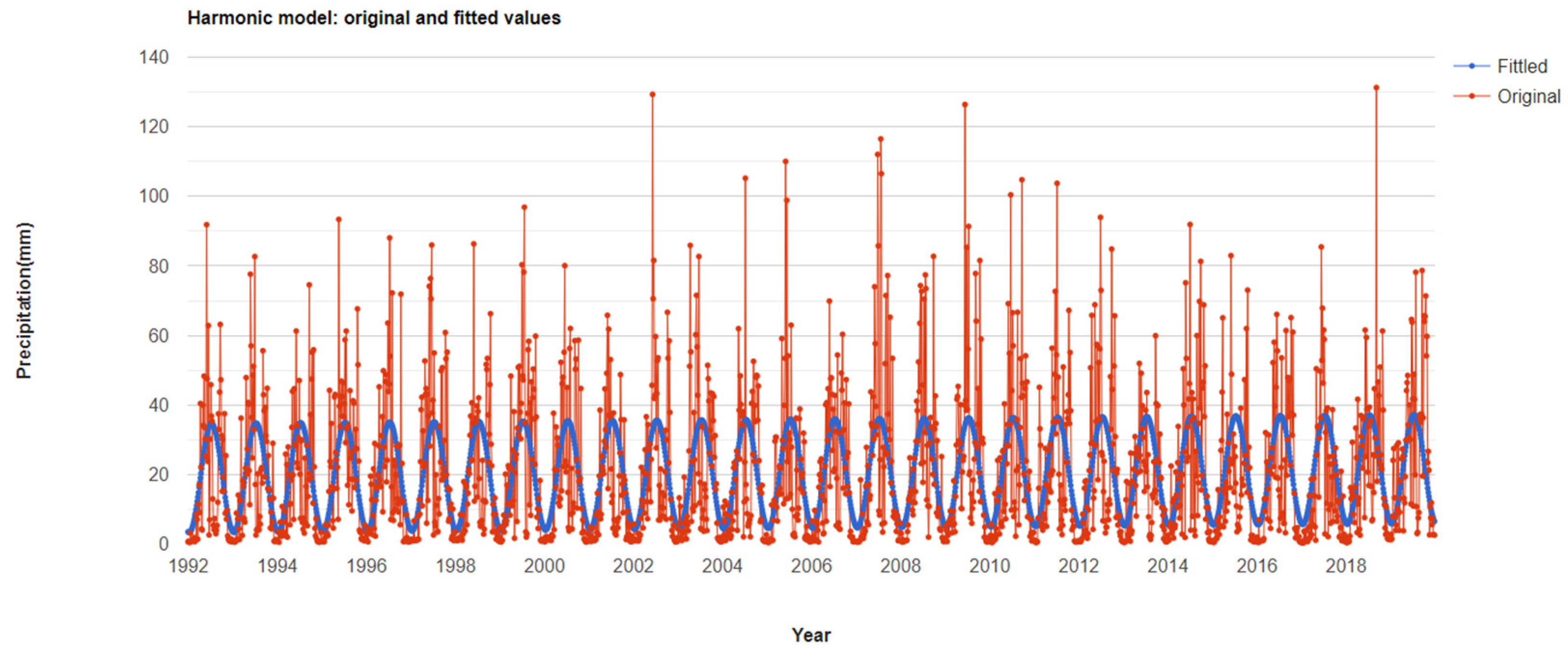
At the beginning of the analysis, the considered study area extent is specified using bounding-box coordinates in the GEE code editor interface. A harmonic model-based precipitation estimation based on daily precipitation for 27 years (from 1992 to 2018) using the CHIRPS precipitation data revealed that the long-term pattern has an upward trend (
Figure 3). Harmonic analysis is suitable for describing and analyzing periodically recurrent phenomena. In fact, this approach is very conducive to reducing complex problems into manageable terms. This entails breaking complicated mathematical curves into sums of comparatively simple components [
38]. Researchers have successfully used harmonic analysis for long-term trend analysis [
39,
40].
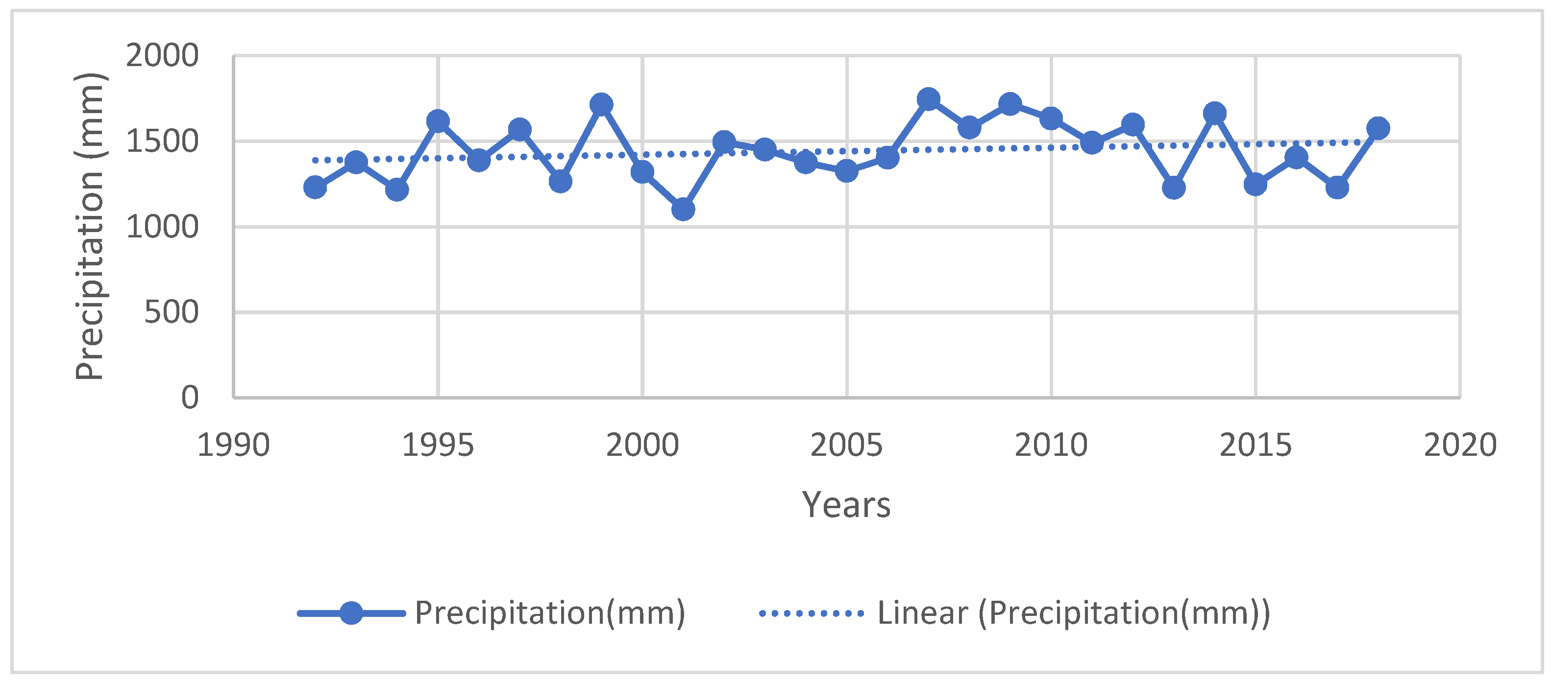
A closer observation of the upper and lower bounds of the fitted curve shows how both gradually increased with increasing time. The upper bound of the fitted curve increased from about 35 mm in 1992 to about 37 mm in 2018 (about a 2 mm increase). The lower bound shows a comparatively higher increasing pattern (about 3 mm) from 3.5 mm to 6.5 mm for the same period. The linear trend based on the yearly total precipitation estimation for the same period also shows a similar upward trend (
Figure 4).
Total yearly precipitation shows inter-annual oscillation (
Figure 4). The linear trend-line shows a positive slope. The fitted line starts from about 1400 mm in 1992 and ends with about 1490 mm of precipitation in 2018. The slope of the trend line is 4.1 with an R-square value of 0.03. So, only 3% of the variance of the yearly total precipitation can be explained with this linear regression model, which is not very significant. Sometimes, a linear regression-based trend could give false results. So, an additional test, the Mann–Kendall trend test, has been performed with yearly total precipitation and the results are presented in the following table (
Table 2).
These results also indicate an insignificant (p-value, 0.34 > 0.05) monotonic trend of 13% (Tau—0.13). So, based on the above analyses, it can be concluded that the precipitation trend based on the whole study area is not statistically significant. The following stages have further investigated precipitation trends for each separate zone created for urban development characterization instead of considering the whole study area as we did for the above analyses.
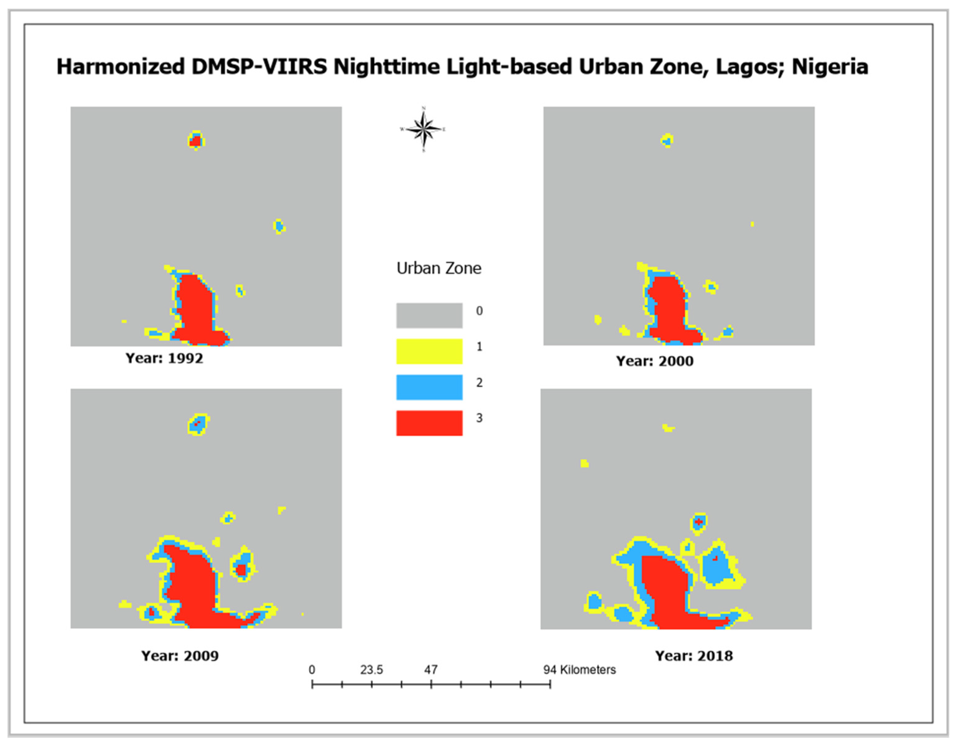
4.2. DMSP-VIIRS Nighttime Light-Based Urbanization Level and Associated Precipitation Estimation
Considering the criteria for urbanization thresholds based on DN values (
Table 1), the study area has been classified into distinct zones. For visual representation and aesthetic purposes, only 4 base years with equal intervals (years) starting from 1992 and ending in 2018 are illustrated in the following figure (
Figure 5).
The area calculation for each individual zone demonstrates that the non-urbanized area (Zone 0) in 1992 was about 9294 square kilometers, but that decreased to about 8573.34 square kilometers in 2018 (
Table 3).
On the contrary, the area coverage for the other three zones, which are actually urban zones (Zone 1, Zone 2, and Zone 3), shows increasing proportions over time, with gradual increments except for Zone 3. For Zone 3, the area coverage in 1992 was 319.06 square kilometers, but was observed as 289.24 square kilometers in 2000. The area coverage for Zone 2 shows the highest increase (324.22 square kilometers) compared to the same area in 1992 and 2018, followed by Zone 1 (294.98 square kilometers), and Zone 3 (101.48 km).
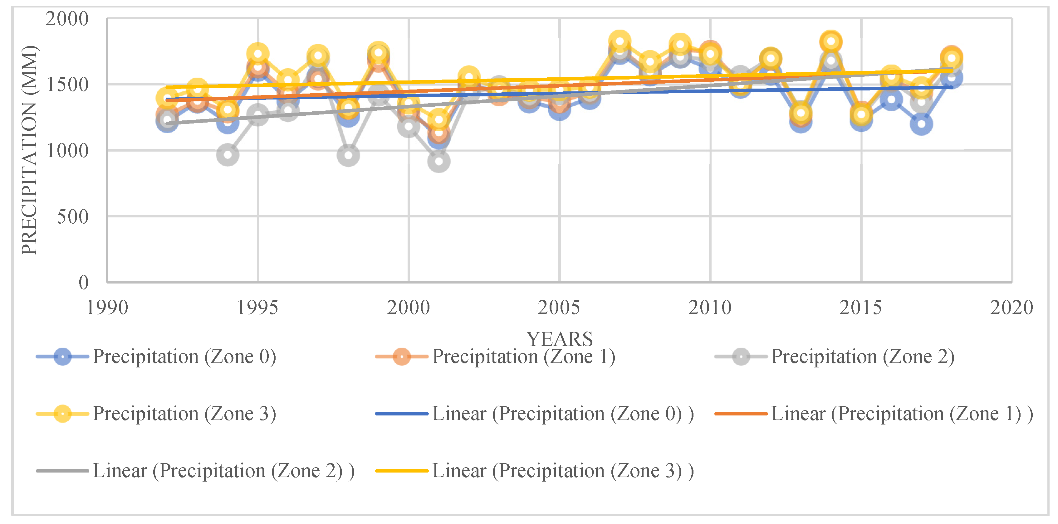
The precipitation calculation has been performed following a systematic method. Initially, after importing the CHIRPS daily precipitation data into the Google Earth Engine, it was aggregated to obtain the early total amount for each considered year. Since we are interested in precipitation for each zone, that aggregated amount has been averaged over the entire zone to obtain the yearly total precipitation for that specific zone. The precipitation calculation for each zone over the study period shows distinct increasing patterns (
Figure 6). Zone 3 (highly urbanized region) has higher precipitation compared to the other two urban zones as well as the non-urbanized zone. However, if we closely observe the trendlines (
Figure 6) together with the data from
Table 4, it is very clear that the curve for Zone 2 (mid-urbanized) has a higher slope than the other zones.
The linear regression coefficients of all trendlines from
Figure 6 are summarized in the following table (
Table 4).
Even though Zone 2 had a higher slope (
Table 4), the higher variability of precipitation (0.13) can be explained for Zone 1.
Similarly, as in the previous stage, the Mann–Kendall trend test has been performed to obtain statistical evidence of an observed pattern in precipitation (
Table 5).
The
p-value for each zone (
Table 5) indicates that no trend is significant. For Zone 1, even though we observed about a 26 % monotonic trend, the associated
p-value (0.06) being slightly higher than the significance level (
p-value 0.05) indicates that it also cannot be considered a statistically valid result.
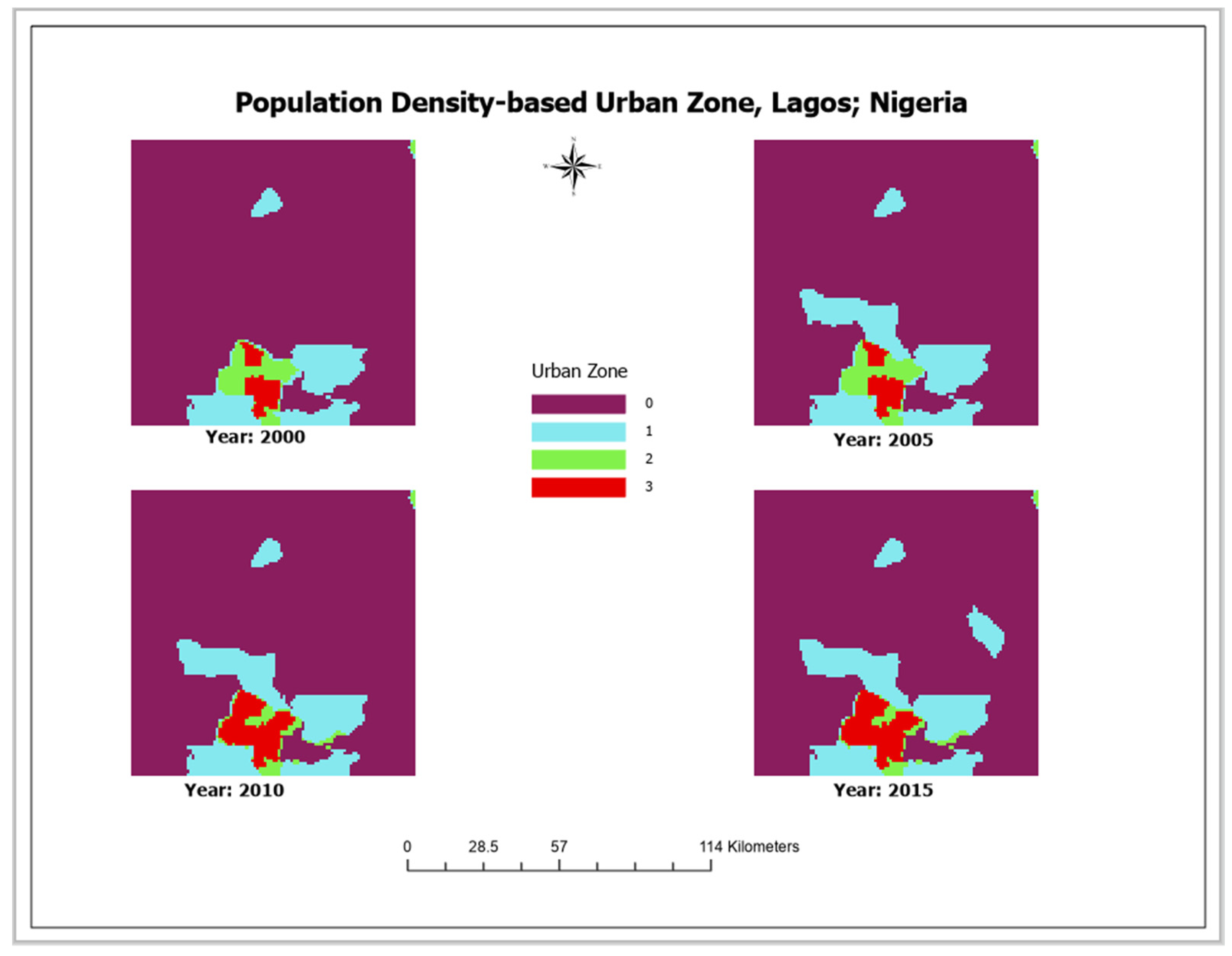
4.3. Gridded Population Density-Based Urbanization Level and Associated Precipitation Estimation
Gridded population density data are available from 2000 to 2020 at five-year intervals (2000, 2005, 2010, 2015, and 2020). However, the study period considered for this study is from 1992 to 2018 (data availability for harmonized nighttime light). This apparent conflict in the timespan was resolved by some assumptions on population density data. For all the years before 2000, the population density was considered as it was for the year 2000. The next population density data available is from 2005, so up to 2004 the population density was also considered as it was in 2000. For 2005 until 2009, the population density was taken the same as it was in 2005. Similarly, from 2010 to 2014, the population density was purposely counted as it was in 2010. Finally, from 2015 to 2018, the population density was deemed as it was in 2015. The urbanization characterization based on the population density criteria (
Table 1) for the available data gives the following distinct maps of the study region (
Figure 7).
The total area calculation (
Table 6) for each year for individual zone shows interesting patterns. Non-urbanized areas decreased to about 552.98 square kilometers (from 8550.12 square kilometers in 2000 to 7997.14 square kilometers in 2015). Zone 1 and Zone 3 show increasing proportions (481.6 and 200.38 square kilometers, respectively) from 2000 to 2015. However, surprisingly, Zone 2 shows a decrease of 129 square kilometers for the considered period.
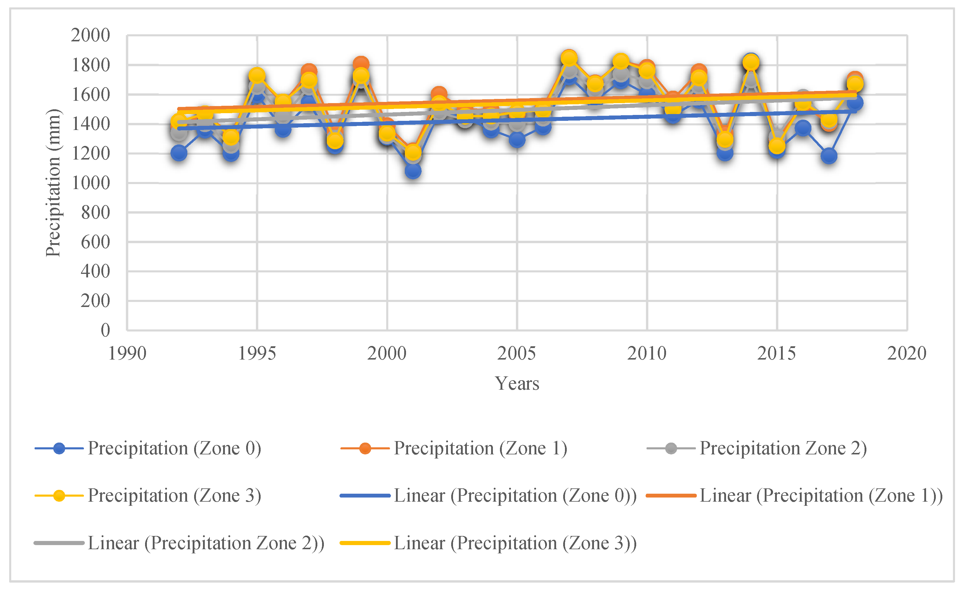
The precipitation estimation based on the population density-based zone data shows that Zone 3 has a higher precipitation rate (slightly higher than Zone 1) than the other zones (
Figure 8). Similar to the previous graph (
Figure 6), Zone 2 demonstrated a higher increasing rate as evidenced by the steeper slope (
Table 7). Also, Zone 0 has the lowest rate as was also the case when considering the nighttime light-based urban characterization.
The Slope and the R-Square values for all the linear regressions from
Figure 8 can be found in the following table (
Table 7).
The R-Square values from
Table 7 are comparatively low, which indicates that these regression models based on only the population density cannot describe the precipitation variability that much.
Again, the Mann–Kendall trend test (
Table 8) is performed to see any possible statistically significant trend in the precipitation variation based on the population density-based zones.
Again, here all the p-value are higher than the significance level. This also means that the apparent monotonic trends observed based on population density are not also statistically significant.
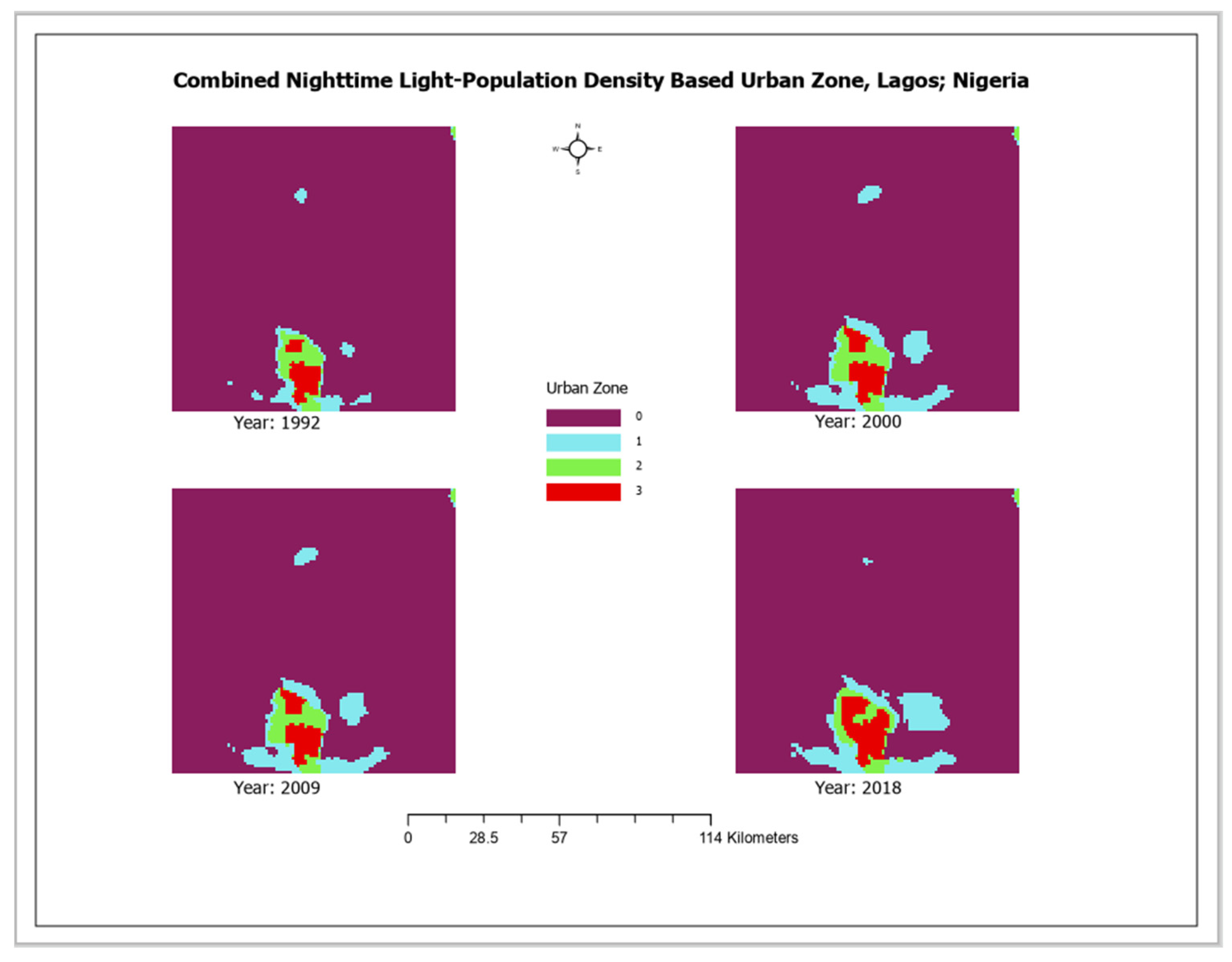
4.4. Combined Nighttime Light and Population Density-Based Urbanization Level and Associated Precipitation Estimation
In the last stage of the precipitation estimation, both nighttime light and population-based urban zones have been considered (
Table 1). The urbanization level based on these criteria gives the following maps (
Figure 9) as the urban development intensity for the considered years.
Again, area calculations for the newly created zones can be summarized in a table (
Table 9). The non-urbanized areas (based on the newly combined criteria) decreased by about 465.26 square kilometers. Although the area for the other zones increased, the increase was not gradual.
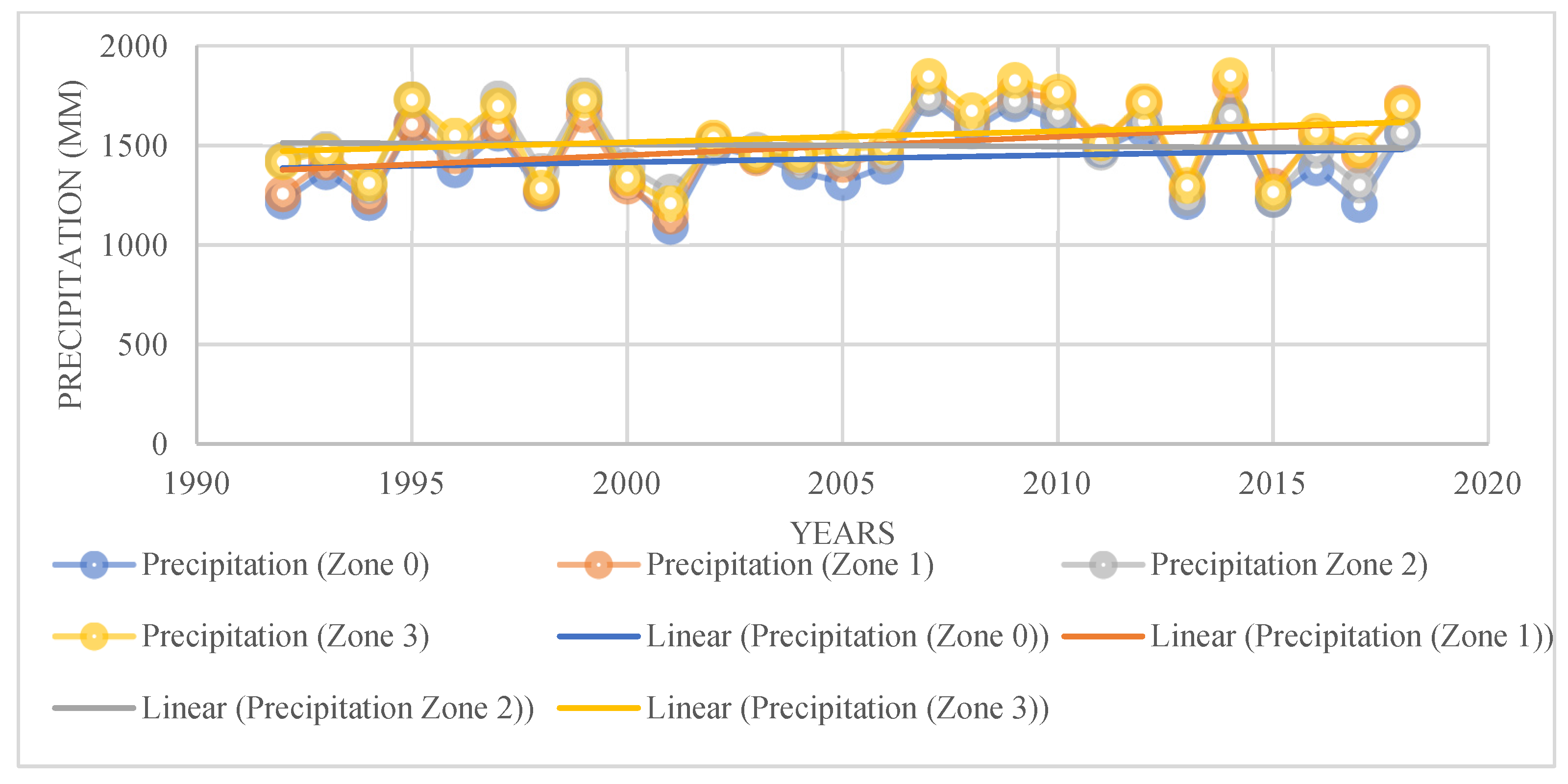
When the plotted precipitation amount was based on the combined criteria, a different kind of pattern emerged (
Figure 10). This time, Zone 0, Zone 1, and Zone 3 have increasing patterns, but the rate of the precipitation increase was higher in Zone 1 as evidenced by a steeper slope (
Table 10). However, surprisingly, Zone 2 showed a decreasing precipitation rate.
Finally, the regression results for
Figure 10 are represented in the following table (
Table 10).
When the combined criteria are considered, Zone 2 starts showing a decreasing slope with a very tiny ‘R-Square’ value. The regression model for Zone 1 could explain about 15% of the precipitation variation. The trendline for Zone 1 shows an increase of about 200 mm (1400 mm to 1600 mm) in precipitation from 1992 to 2018.
Again, the Mann–Kendall trend test (
Table 11) is applied to estimate the statistical evidence of the precipitation trend.
The Mann–Kendall trend test results based on the combined criteria are very interesting. Zone 1 shows statistically significant (p-value of 0.03) results. It also exhibits the highest monotonic trend of 29%. Zone 2 exhibits an apparent negative trend, although it is not statistically significant.
5. Discussion
An urban area is not homogenously developed. Some parts of it might be densely developed and congested with buildings, or populations. Previous research has contributed to exploring and explaining urban-induced precipitation while considering the whole area rather than explicitly considering the level of urbanization. This study made an innovation in urban-induced precipitation research by incorporating multi-source urban information. Considering the nighttime light and population density data for urban characterization and analyzing the associated satellite precipitation data CHIRPS, this study also showed how remote sensing and satellite information are advancing the urban research domain.
When the nighttime light and population density data have been used individually to demarcate urban development-based zones, the associated precipitation variation did not show statistically significant patterns. There could be two reasons behind this. First, it could be solely due to the fact that neither of these indicators (nighttime light and population density) is individually capable of meaningfully representing urban development in such a way that is conducive to conducting urban effect-related studies. Secondly, it could be that we need to consider a longer time period if we want to see a statistically significant precipitation variation based on a single factor. However, surprisingly, when these two factors are combined for an urban characterization, they showed very promising patterns, which are valid based on statistical thresholds. In this case of urban characterization, Zone 1 showed a significant pattern as evidenced by the Mann–Kendall trend test results. Zone 1 is the transition region from non-urbanized areas (Zone 0) to higher urbanized areas (Zone 2 and Zone 3). Based on the above-mentioned multi-faceted analysis, instead of core (Zone 3) and adjacent mid-urbanized (Zone 2) areas, transition areas with low urbanization (Zone 1) experienced increasing precipitation.
Another important aspect of these analyses is that we observed differences in the results when considering the nighttime light and population density data individually and then using the combined method. The reason is that when the nighttime light-based urban zones are created, they are not the same as when the population density-based zones are created. There are areas that could have a higher population density but with moderate or lower nighttime light. In order to capture this fact, the final analysis has combined them to obtain a robust urban characterization where both followed specific thresholds.
5.1. Significance of the Research
This study is unique in the sense that instead of just considering the whole area for an aggregate level analysis, this study has proceeded further and divided the whole study area into specific zones of urban development based on pre-defined criteria of well-established variables. Urban development quantification and the estimation of associated precipitation are the innovations of this study. The above-mentioned significant results could be a good indication for other researchers, who, in the future, could characterize urban development based on nighttime light and population density data for urban-induced precipitation analysis.
However, one important question needs to be answered, which will eventually provide the basis for this research. How reliable is the CHIRPS precipitation data for long-term trend and spatial variation analyses? To answer this question, we need to see what other researchers are doing and how they are doing it. A number of research has been conducted to assess the adequacy of the CHIRPS precipitation data, and the results showed satisfactory reliability of the CHIRPS precipitation data. While studying in Xinjiang, China, ref [
41] compared two long-term and high-resolution satellite precipitation datasets (PERSIANN-CDR and CHIRPS). Their findings reported that even though both datasets showed similar agreement with gauge precipitation data, CHIRPS outperforms PERSIANN-CDR with smaller errors and biases. In addition, they concluded that CHIRPS is more accurate for estimating the spatial distribution of average monthly and annual precipitation. In a very similar study employing these two datasets, ref [
42] suggested that remote sensing/satellite precipitation data can reliably be used in inaccessible regions where there are not enough observational data and/or available data is temporally incomplete. Ref [
43] also found that the CHIRPS data can adequately capture the spatial distribution of precipitation. The CHIRPS precipitation data have also been found effective in drought identification and monitoring. Ref [
44] have utilized the CHIRPS data for drought monitoring in Bundelkhand, India. In a detailed study of the spatio-temporal rainfall trend analysis, ref [
45] evaluated several satellite rainfall products and CHIRPS was found to be the best product for rainfall variation capturing. Ref [
46] have used CHIRPS for long-term spatio-temporal trends and the variability of rainfall over eastern and southern Africa. They reported that CHIRPS can provide reliable, high spatial resolution rainfall information that can complement the sparse rain gauge network.
From the above references, it is evident that the CHIRPS data can provide satisfactory results if not best for long-term trend analysis, specifically in regions with sparse/incomplete gauge precipitation data. So, it was an appropriate decision to consider CHIRPS in this study. The differences between the current study and the above-mentioned studies are in the study focus and the way it has been performed. The current study focuses on the spatio-temporal responses of precipitation due to urbanization by classifying the study area into distinct zones based on nighttime light and population density, and then combining them, whereas others have focused on estimating spatio-temporal variations for an area at an aggregate level.
5.2. Limitations of the Study
Every kind of research is very likely to have one or several limitations and this study is not an exception to that. The first limitation is with the data. Even though a suitable number of references have been provided for the relevancy of the satellite-based precipitation data CHIRPS for spatio-temporal dynamics investigation, it would be better if in situ long-term precipitation data were available for all four zones. There were also limitations with the nighttime light and population density data. The nighttime light data are available from 1992, which restricts how far back we can go in terms of analysis. The gridded population density data is available from 2000 to 2020 at five-year intervals (2000, 2005, 2010, 2015, and 2020). This poses the main limitation of this study. Since the study period for this research is from 1992 to 2018, the population density for 2000 was assumed as it was for 1992 as well as some other assumptions due to analytical requirements (detailed in
Section 3).
5.3. Future Research Direction
This research is part of a long-term project. In the next stage of this research, we will attempt to overcome some of the limitations described above, if possible. Also, precipitation trends for other study areas from diverse climatic settings will be investigated to acquire an understanding of their underlying urban-induced precipitation patterns based on different levels of urbanization.
6. Conclusions
Urban-induced precipitation is multifaceted and has considerable relevance to urban design, local water supplies, hydrological design, and so on. Previous studies have focused on quantifying the urban effects on precipitation at the aggregate level, considering the whole urban area at a time, but the differences in urban development intensities in a certain urban area were not considered. This study is focused on filling that gap and bringing that concern to the whole urban research community.
Initially, this study has considered the whole study area (traditional approach) and estimated the long-term (1992 to 2018) harmonic model-based precipitation trends with daily CHIRPS precipitation data and yearly total precipitation patterns for the same study period. Both analyses showed increasing precipitation patterns for the study area, but the trend in yearly total precipitation was not significant based on the Mann–Kendall trend test.
In the next stage of this research, harmonized DMSP-VIIRS nighttime light data and global population density data will be used to characterize urban development by considering them individually and then finally by combining them based on pre-defined thresholds. A total of four zones were created: Zone 0 refers to non-urbanized areas and Zone 1, Zone 2, and Zone 3 refer to low-urbanized, mid-urbanized, and highly urbanized areas, respectively. The Mann–Kendall trend test for each stage of the precipitation analysis showed that only urban characterization based on combined DMSP-VIIRS nighttime light and population density was able to capture a significant precipitation trend. Specifically, based on the combined criteria, Zone 1 had a monotonic upward (Tau—0.29) precipitation trend with a 0.03 significance level.


