Review

Review of Current Software for Analyzing Total X-ray Scattering Data from Liquids

by
Leighanne C. Gallington
1,
Stephen K. Wilke
1,
Shinji Kohara
2 and
Chris J. Benmore
1,*
1
X-ray Science Division, Argonne National Laboratory, Lemont, IL 60439, USA
2
Quantum Beam Diffraction Group, Center for Basic Research on Materials, National Institute for Materials Science, 1-2-1 Sengen, Tsukuba 305-0047, Japan
*
Author to whom correspondence should be addressed.
Quantum Beam Sci. 2023, 7(2), 20; https://doi.org/10.3390/qubs7020020
Submission received: 4 May 2023 / Revised: 27 May 2023 / Accepted: 2 June 2023 / Published: 20 June 2023
(This article belongs to the Special Issue Quantum Beam Science: Feature Papers 2023)

Abstract

:
The popularity of the pair distribution function (PDF) analysis of X-ray total scattering data has steadily grown as access to ex situ synchrotron data has expanded. Due to the broadening of the PDF user community, there is a growing demand for software that can be used to extract PDFs and is accessible to non-expert users. While user-friendly options have been developed over the past decade for fast, streamlined data analysis, care must be taken in both processing the data and understanding any limitations, especially in the case of liquids. In this review, the same scattering data are analyzed using different total X-ray scattering software, in order to compare the accuracy of the extracted structure factors and associated pair distribution functions. The goal is to assess the best practices for extracting the most accurate liquid data for each software package. The importance of absolute normalization and the application of the most appropriate corrections are emphasized via quantitative comparisons between liquid sulfur and water. Additionally, an awareness of the competing conventions used to define the PDF in crystallography and liquids/glasses is crucial for both the downstream analyses of the data and a comparison with the previous results in the literature.

1. Introduction

The popularity of the pair distribution function analysis of X-ray total scattering data has steadily grown as access to ex situ synchrotron data has expanded in recent years. Additionally, brilliance-enhancing upgrades to synchrotrons around the globe enable the rapid acquisition of increasingly large in situ total scattering datasets. Due to the broadening of the PDF user community, there is a growing demand for software that can be used to extract PDFs and is both accessible to non-expert users and capable of batch and/or automated data processing. While user-friendly options have been developed over the past decade for fast, streamlined data analysis, care must be taken in processing the data, understanding any limitations, and comparing it to previous results in the literature. Special care must be taken in the case of liquids and glasses, where the measured signal can be in the same order of magnitude as the background, and features of interest can be swamped by artifacts. In this review, the same set of liquid scattering data are analyzed using different available total X-ray scattering software, in order to compare the accuracy of the extracted structure factors and associated pair distribution functions. The software packages are utilized following the available guidance a newcomer would be given in order to highlight pitfalls and establish the best practices for obtaining reliable results. This work is a tribute to the work of Prof. Adrian Wright, a world-renowned expert on glass diffraction, who sadly passed away during the writing of this manuscript.

2. Fundamentals of Extracting Structure Factors and Pair Distribution Functions from X-ray Total Scattering Data

Water and molten sulfur data were collected at the Advanced Photon Source using the high-energy beamline 6-ID-D, which is optimized for pair distribution function measurements of liquids, glasses and amorphous materials. Experimental details have been described previously by Benmore et al. [1,2]. The X-ray data were obtained from an amorphous silicon flat-plate area detector constructed from several panels containing a large array of pixels. These types of CsI scintillation detectors are known to have a high dark current, which is measured with the beam off, immediately prior to sample measurement. The underlying dark current produces a pixel offset, which is directly subtracted. The varying pixel response is corrected with an appropriate gain map obtained using a multiplicative flat-field correction factor. Given that there are typically up to ~8 million pixels on a 2D detector, some outliers remain in the diffracted image, either from low or non-counting pixels or high-counting trapped excited states [3], which are typically masked in the azimuthal integration procedure. Efforts to minimize these effects experimentally and correct for them have been discussed elsewhere [2]. For monochromatic X-ray beam experiments, the integrated data are converted from scattering angle to momentum transfer using a crystalline calibration standard such as LaB6 or CeO2. The main aim of this paper is to discuss the subsequent corrections and normalization procedures typically applied in the currently available total X-ray scattering software used to extract the total X-ray structure factor and associated pair distribution function.
By far the most important technique used to analyze liquid scattering data is data normalization, after appropriately scaled background subtractions. The measured intensity needs to be scaled to the sum of the squared X-ray form factors plus Compton scattering, C(Q) (referred to as the self-scattering) [4,5]. To achieve this, multiple effects need to be taken into account, in order to yield the normalized electron density I(Q) in absolute electron units. These effects include geometry, polarization, fluorescence, multiple scattering and attenuation by air, filters, detector and the sample [6,7,8,9]. Firstly, standard geometric corrections for the specific experimental arrangement and beam polarization should be applied. Fluorescence above K-edges are usually assumed to be isotropic in correction procedures, but are unpolarized and have a different wavelength to the incident beam, so often have a more complex shape. Notably, for high-energy X-ray scattering (>60 keV), most angular dependent corrections are minimized, except for the oblique incidence correction, which becomes problematic at high-Q values due to the longer path length through the detector scintillation material at high angles [10]. For lower energy X-ray, i.e., laboratory sources, Q-dependent attenuation and multiple scattering effects are generally complex and care is needed when estimating their magnitude and shape (usually using a geometry-specific Monte Carlo-type simulation [8,9,11]). This is essential in order to ensure that the correct Q-dependent background subtraction factor is applied (and subsequent normalization). By design, high-energy X-ray diffraction experiments help to minimize absorption effects, and accurate estimations can be obtained using the calculations of Paalman and Pings for flat-plate and cylindrical geometries [6]. A general rule of thumb is to keep the sample attenuation below ~20% to avoid having to perform difficult multiple scattering corrections.
The Compton wavelength depends on the scattering angle [12], and a power law can be used to correct for the energy-dependent absorption in the detector. The Klein–Nishina correction accounts for the energy dependence of the Compton scattering due to relativistic effects and can be approximated by the Breit–Dirac equation using a power of two [2,13]. A summary of the magnitude of each of these individual corrections using 100 keV X-ray data has been described by Skinner et al. [2]. The normalized electron density for molten sulfur and water using atomic form factors are shown in Figure 1. We note that traditionally molecular liquids were normalized per molecule [14,15,16], but here we normalize them per atom, since the majority of modern total X-ray scattering software assumes atomic (independent atom) form factors.
Although atomic form factors are accurate at high-Q values, the hydrogen bonding between water molecules (and other hydrogen bonded organic liquids) is known to modify the intramolecular electron density, compared to that of the isolated atoms. To account for this, modified atomic form factors (MAFF) have been successfully used to describe the resulting change in the electron density within the molecule.
The MAFF f α 0 Q is defined as follows:
f α Q = f α 0 Q 1 a O z α e Q 2 / 2 δ 2
where f α 0 Q is the atomic form factor of the isolated atom species α , and z α is the total number of protons on the atoms of species α . In the case of water the α O and α H terms are −1 and +0.5, respectively, corresponding to the transfer of 0.5 electrons from each hydrogen towards the oxygen and δ = 2.0 Å−2 [17,18].
A normalized total scattering X-ray structure factor S(Q) is typically defined as follows:
S Q 1 = I Q α c α f α 2 Q C Q α c α f α Q 2
where cα is the concentration of atoms of type α. Using the Hannon–Howells–Soper notation [19,20], the total structure factor is related to the pair distribution function g(r) through a Sine Fourier transform,
g r 1 = 1 2 π 2 ρ 0 Q m a x Q S Q 1 s i n Q r r M Q d Q
where M(Q) is an optional modification function, and ideally equals unity. The differential correlation function, with the bulk density, ρ, removed is defined as follows:
D r = 4 π ρ r g r 1
There are stringent normalization checks for liquid structure factors normalized onto an absolute scale using the X-ray form factors. These include S(Q → 0), S(Q → ∞), G(r → 0) and I(Q) > 0. With regard to the low Q limit, from Equation (2), it can be seen that S(Q → 0) becomes more negative for systems that contain elements with a large difference in the number of electrons. For a homogenous, monoatomic liquid at equilibrium, the S(0) limit is directly related to the isothermal compressibility χ T [21,22] via Equation (5).
S Q = 0 = ρ χ T k B T
The isothermal compressibilities for water and molten sulfur are 5 × 10⁻¹⁰ m2/N and 4 × 10⁻⁴ m2/N, respectively [23,24,25,26], which correspond to S(0) values of zero for elemental molten sulfur, and −0.98 for water using atomic form factors and −2.0 using MAFF’s. In addition, by definition, at high-Q, S(Q → ∞) = 1. See Figure 2.
Provided that the extracted S(Q) meets the consistency checks in the reciprocal space and the appropriate form factors have been used in the data reduction, the Sine Fourier transformation of S(Q)yields a g(r) with low-r oscillations around zero, i.e., in the unphysical region, below the closest atom–atom distance. Equivalently, the low-r data in D(r) oscillates around the −4πρr density line, as shown in Figure 3. This holds for the case of elemental sulfur, where the atomic form factor represents a good approximation of the electron density. However, it only holds for water if the appropriate MAFF’s are used. If atomic form factors are used to obtain S(Q), there will be a mis-match in the electron density at low-r, since the number of electrons displaced from the H nucleus is a large percentage of the total number of electrons in the system. In addition, there is a low-r (non-zero) contribution of the O–H partial below the first O–O peak. Even then, the low electron density of water makes the accurate extraction of S(Q) difficult to achieve, since the Compton scattering and other backgrounds are large compared to the rapidly decaying form factors.
A major problem with the Fourier transformation of diffraction data arises from the finite Qmax (≠∞), and to a lesser extent, the fact that Qmin ≠ 0. The consequence of a finite Qmax is the introduction of a step function into the Fourier transform if S(Qmax) ≠ 1, resulting in truncation oscillations in g(r). Qmin, on the other hand, is often extrapolated to the S(0) limit, either by linear extrapolation or Lorentzian fitting [27]. The maximum Q-value of the measured S(Q) determines the real-space resolution limit of the pair distribution function, g(r) [2,22]. This is a primary reason why high-energy X-ray diffraction is preferred for X-ray PDF studies, since it allows access to the highest momentum transfers. For analysis purposes, the truncation problem is commonly treated by truncating at a node where S(Q) = 1, and/or introducing a modification function that dampens the measured S(Q) smoothly to unity at Qmax before Fourier transformation [28]. Modification functions, such as the commonly used Lorch function [29], tend to reduce truncation oscillations at the expense of artificially broadening the sharpest features in g(r).
For a system in which the density is well known, the Krogh-Moe and Norman technique [30,31] can be used to normalize S(Q), by setting the region below the closest approach between the atoms in D(r) to the density line. In some cases in the literature, this artificially corrected real-space function has been Fourier back-transformed into the Q-space and shown as experimental data, concealing the real quality of the measurement [32,33]. This approach hides errors that could be due to, for example, severe Q-dependent fluorescence, sample absorption or multiple scattering effects. This is because long-wavelength systematic errors in the X-ray measurement typically appear at low-r in the pair distribution function, particularly below the first real peak, and provide an indication of the accuracy of the experimental data in real space. If the transform only shows small truncation errors in this region, then the data can be claimed to be of reasonably good quality. However, as pointed out by Wright in 1993 [32], some authors, either knowingly or unknowingly, sometimes disguise or do not show data in this region in order to give the illusion of higher-quality data. Furthermore, Wright has described using data in the low-r unphysical region below the first peak to fix any mismatches in the data as “a particularly devious technique” and has said that “such data must be treated with the utmost suspicion” [32]. Thirty years later, this technique has become the basis of some of the software packages used in this review.
However, in practice, the purist view of data analysis has to be moderated to some extent, because if S(Q) does not tend exactly towards unity at Qmax, a step function will be Fourier transformed, thus introducing additional oscillations into g(r), i.e., Fourier artifacts that are unrelated to the data quality. Since every experimental dataset has some degree of systematic error, it is commonplace for the experimental S(Q) to diverge, either positively or negatively, at the highest Q-values. The work of Skinner et al. [2] confirms this behavior for high-energy X-ray experiments using flat-plate area detectors, since most corrections to the data have very similar diverging shapes, which can be readily approximated using a quadratic-type equation. Therefore, in most data analysis software packages, there are one or more parameters used to enforce the S(Qmax) = 1 constraint, other than simply truncating at a node in which S(Q) intersects with 1. This may be considered reasonable if the correction is small, say a few percent, but if the correction becomes large, it is likely masking a larger problem. The nature of the correction used should also be considered with care.
An alternative use of the Fourier back-transform mentioned earlier is to employ it as a test of the accuracy of the correction procedures in the Q-space, by comparing it directly to the measured data [34], as shown in Figure 4. Comparing the measured data quality in the Q-space to the 3D atomistic models is preferred because the magnitude of both systematic and random errors on the diffraction pattern can be assessed.
The correct normalization of the X-ray diffraction data has strong implications for interpreting the structure of the liquid. While the PDF is in some sense fairly robust, such that the atom–atom distances are likely to be correct, the extraction of absolute coordination numbers, nαβ [34], is highly sensitive to the absolute normalization. Coordination numbers are determined by integrating the following function:
n α β = r 1 r 2 4 π ρ r 2 c β g α β r d r
where nαβ represents the number of atoms of type β that reside between distances r1 and r2 from an atom of type α at the origin; cβ is the concentration of atoms of type β; and gαβ(r) is the Faber–Ziman partial pair distribution function [35] describing αβ pair interactions. Firstly, it should be noted that nαβ can only be reasonably extracted if the αβ pair interactions represent a sizeable percentage of the X-ray scattering. Secondly, a significant error in the absolute normalization of the X-ray data, or bulk density, will be magnified in this integral and could yield chemically unrealistic coordination environments.
For oxide systems, bond valence theory enables specific cation–oxygen distances (which tend to be robust in g(r)) to be correlated with particular polyhedral environments, i.e., tetrahedral, octahedral, etc., based on effective ionic radii [36]. For molecular liquids, the first few peaks in the intra-molecular structure can be used to obtain absolute normalization [37]. In most cases, including those in which homopolar bonding occurs, confirmation that the normalized g(r) represents a chemically realistic structure can be obtained via the use of so-called “big-box” (>1000 atoms) atomistic modeling, such as Reverse Monte Carlo (RMC) [38,39] or Empirical Potential Structure Refinement (EPSR) [40,41]. Although not definitive, these atomistic models will help to determine whether the X-ray data are properly normalized when chemically realistic constraints are imposed. There is the possibility of scaling the S(Q) (or g(r)) to improve the fit in these programs. Hopefully, this is a small adjustment (say < ±5%), as it indicates that either one or more of the correction factors has not been correctly applied in the analysis, or there is significant systematic error in the measurement or normalization process. “Small-box” (<50 atoms) modelling software, which includes programs such as PDFgui and TOPAS, inherently expect a scaling factor to be applied to D(r) as part of the real-space Rietveld refinement process [42,43,44]. This approach works adequately for highly crystalline materials in which the lattice structure and therefore the bulk density are known; however, it is problematic for liquids and glasses in which the local coordination numbers are unknown. For example, in oxides, the local coordination of melts is known to be substantially lower than their crystalline counterparts [45].
Figure 5 shows the EPSR fits for molten sulfur [46] and water [17], together with the corresponding running coordination number as a function of distance for the well-determined S–S and O–O coordinations, which dominate the signal and the ill-determined (weakly weighted) O–H coordination.

3. Methods and Discussion of PDF Extraction Software Process and Available Corrections

3.1. Original Analysis

For our previous analyses discussed above, data reduction and processing were performed as described by Skinner et al. [18]. Detector calibration, the application of flat fields, the masking of bad pixels, and the azimuthal integration of diffraction images for water and sulfur were performed in FIT2D [47]. Then, one-dimensional X-ray diffraction patterns were exported in constant Q−1) bin format. Structure factors and differential correlation functions for liquid water (Q = 0.5–20 Å−1) and molten sulfur (Q = 0.5–28 Å−1) were extracted from one-dimensional X-ray diffraction patterns using PDFgetX2 [48]. A scale factor of 1 was used for the sample background in each software package. Ideally, the sample transmission would be measured, and the appropriate attenuation factor used here in lieu of the calculated absorption correction listed below. Corrections for oblique incidence and polarization were applied within the program. Corrections for Breit–Dirac, sample self-absorption and multiple scattering were also applied. The parameters for energy-dependent Compton scattering (1/E quadratic) and fluorescence were refined during the optimization of S(Q). The fluorescence correction implemented in PDFgetX2 takes the form of a constant offset, and was actually used in our example cases to correct for drift in the detector dark current. The Q range for the optimization of F(Q)→ 0 was set to 10 to 20 Å−1 for water and to 20 to 26 Å−1 for sulfur. A Lorch modification function was applied to the reduced structure factor, F(Q). Pair distribution functions were calculated from the differential correlation function using Equation (4).

3.2. Fast PDF Extraction Software

For our comparison of fast PDF extraction software, a simplified data reduction and processing procedure was followed in order to highlight deviations from the carefully undertaken “original” analysis described above. Detector calibration, the masking of bad pixels, and the azimuthal integration of diffraction images for water and sulfur were performed in GSAS-II [49]. Data were exported in both constant Q−1) bin format and constant 2θ bin format. Structure factors for liquid water (Q = 0.5–20 Å−1) and molten sulfur (Q = 0.5–26 Å−1) were extracted from one-dimensional X-ray diffraction patterns using GSAS-II, PDFgetX2, PDFgetX3, LiquidDiffract, GudrunX, and BL04B2anaGUI [48,49,50,51,52,53]. Pair distribution functions (PDFs) were subsequently obtained via the sine Fourier transformation of the reduced structure factor, which was performed natively in each software package. In PDFgetX2, GSAS-II, and PDFgetX3, which are heavily used by crystallographers, the pair distribution function, G(r), contained in their *.gr files is defined according to the convention specified in Egami et al. [54]:
G r = 2 π 0 Q m a x Q S Q 1 s i n Q r M Q d Q
where M(Q) is the modification function (usually Lorch). This pair distribution function, G(r), is equivalent to the differential correlation function, D(r), in Hannon–Howells–Soper notation. Additionally, these programs output the reduced structure function, F(Q), into *.fq files, where F(Q) is defined as follows:
F Q = Q S Q 1
In contrast, LiquidDiffract and GudrunX, which are aimed at the liquids and glasses communities, utilize the Hannon–Howells–Soper formalism for the pair distribution function [19,20] shown in Equation (3). For consistency, we will continue to use Hannon–Howells–Soper notation, and will therefore denote the PDFs obtained using PDFgetX2, GSAS-II, and PDFgetX3 as D(r) in our review. A summary of the corrections and parameters used for all the different software packages are given in Table 1.

3.2.1. PDFgetX2

Structure factors and differential correlation functions were extracted for water and molten sulfur using PDFgetX2 version 1.0. The sample background data scaling, which can be set and adjusted manually in PDFgetX2, was set to 1. Corrections for oblique incidence and polarization were applied within the program. In this example, the corrections for Breit–Dirac, sample self-absorption and multiple scattering were also omitted. The parameters for energy-dependent Compton scattering (1/E quadratic) and fluorescence were refined during the optimization of S(Q), as with our previous analyses. These parameters should be zero in an ideal experiment; however, here they are simply used to correct any remaining systematic errors. Due to the fact that S(Q) was not oscillating around 1, a flat line offset for water was manually set to 2.5 × 10⁵ in lieu of the refined fluorescence parameter. The Q range for the optimization of S(Q) → 1 was set to 10 to 20 Å−1 for water and to 20 to 26 Å−1 for sulfur. A Lorch modification function was applied to F(Q). Pair distribution functions were calculated from the differential correlation function using Equation (4).

3.2.2. GSAS-II

Structure factors, differential correlation functions, and pair distribution functions were extracted for water and molten sulfur using the PDF calculation module within the GUI of GSAS-II version 5509. The use of versions 5509 or later is required for the correct normalization of the Fourier transform, following the discovery of this flaw during the writing of this review. The sample background multiplier, which was set to (the default) −1, was not refined. Formula volumes (n/ρ0) were calculated for water (29.969 Å3) and molten sulfur (29.272 Å3) and used in lieu of those calculated by GSAS-II. The refined parameters included a flat background, an offset that can correct for effects such as fluorescence, which is assumed to be negligible for these samples at high energies, and drift in the detector dark current; the Ruland width [55], to correct for Compton scattering (although this should not be significant for experiments using high X-ray energies); and the background ratio, an empirical correction that forces S(Q) to approach 1 at a high Q. The desired Qmin was set by changing the minimum 2θ of the associated powder item in the project. For the S(Q) optimization to oscillate about 1, the scaling Q range was set to Q = 10 to 20 Å−1 for water and to 15 to 26 Å−1 for sulfur. A Lorch modification function was applied to F(Q), but the option to suppress low-r ringing in the Fourier-transformed D(r) was not used. The pair distribution function, labeled g(r) in the GUI, was exported from the GSAS-II project file by using the GSASIIscriptable API.

3.2.3. PDFgetX3

Structure factors and pair distribution functions were extracted for water and molten sulfur using PDFgetX3 version 2.1.1. The sample data, the corresponding background data and scaling, as well as the desired Q range, were specified in a custom configuration file. Qmaxinst was set to be the same value as Qmax for each dataset. Corrections for Compton scattering, the drift in the detector dark current, and the fluorescence were automatically performed by the software, and could not be disabled or manually adjusted. The user-controlled optimization of the pair distribution function can be performed using the built-in tuneconfig() function, which enables the interactive adjustment of the Q range, background scaling, Qmaxinst and rpoly, which is the minimum r cut-off for physically meaningful correlations in the PDF. PDFs were generated using both the default value of 0.9 and a manually selected value of 1.5 for rpoly. rpoly and Qmaxinst determine the order of the correction polynomial, n + 1, applied to the structure factor [50]:
n = Q m a x i n s t r p o l y π  
This ad hoc correction was automatically performed by the software, and could not be disabled or manually adjusted, aside from rpoly and Qmaxinst. The user-controlled optimization of the pair distribution function can be performed using the built-in tuneconfig() function, which enables the interactive adjustment of the Q range, background scaling, Qmaxinst and rpoly,. Differential correlation functions were generated using both the default value of 0.9 Å and a manually selected value 1.5 Å for rpoly. These correspond to the correction polynomial degrees of 6.7 and 11.2 for water, and 8.4 and 13.4 for sulfur. It is of note that all the functionality described is also readily accessible via an interactive GUI client, xPDFsuite [56]. Pair distribution functions (g(r)) were calculated from D(r) using Equation (4), employing the low-r slope (−4πρ0) to estimate the density in lieu of the known atomic number densities. Values of 4πρ = 0.06 and 0.13, which correspond to atomic number densities of 0.00477 and 0.0103, were used for sulfur and water, respectively. These values are roughly an order of magnitude lower than expected.

3.2.4. LiquidDiffract

Structure factors and pair distribution functions were extracted for water and molten sulfur using LiquidDiffract version 1.11. The use of version 1.11 or later is required for the correct Compton scattering corrections, following the discovery of a software bug during the writing of this review. Data were read into the GUI, re-binned to a user-specified Q bin size, and extrapolated to Q = 0. The background scaling was set to 1, and the atomic number densities (ρ0) were set to 0.1003 and 0.0334 atoms/Å3 for water and sulfur, respectively. These parameters were not refined. The desired Q range was set in the GUI, and the Lorch modification function was applied. The Faber–Ziman formulation of S(Q) was used for this extraction. The structure factor was optimized using an rmin cut-off of 0.5 Å for 80,000 iterations, using the method of Eggert et al. [57], in which the difference between the observed and modelled behavior of D(r) below rmin is Fourier transformed into reciprocal space, and subtracted from the measured I(Q).
Correction for Compton scattering is performed by the software using tabulated values from Hubbell et al. [4], but is not visible to, or adjustable by the end user from within the GUI. Correction for fluorescence is not currently implemented, but is planned for a future update. All processing and optimization routines are accessible for import into external Python code. For comparison with other PDF extraction packages, D(r) was back-calculated from the *.gr files by rearranging Equation (4).

3.2.5. GudrunX

Prior to the GudrunX calculation of structure factors and pair distribution functions, 2θ-binned I(Q) data were manually corrected for detector attenuation and oblique incidence [2], since these corrections are not available within the program. The data were then imported into GudrunX, and the Q range was set as 0.45–20 Å−1 for both water and sulfur. The parameters for bremsstrahlung, pertinent for a lab-based X-ray source, were not used. Scattering data were normalized to <F>2, a Breit–Dirac factor of 2 was used for Compton scattering, and Krogh-Moe and Norman normalization was enabled. Background scaling was set to 1. Mass densities were set to 1.0 and 1.8 g/cm3 for water and sulfur, respectively. The factors used to modify the multiple and Compton scattering were both set to 1. The fluorescence correction was manually adjusted to optimize the fit of I(Q) to the self-scattering.
GudrunX also offers parameters for the so-called “top hat” convolution [58], which is a Fourier space filtering method used to remove any residual long-wavelength background in S(Q). The top hat convolution uses two parameters: (1) rmin, which is set to be smaller than the first atomic pair correlation in real space, and (2) QT, which is the threshold at which frequencies are to be suppressed in S(Q) in order to remove the residual background. Ideally, the top hat convolution is not necessary, and the S(Q) obtained before and after the top hat will be nearly identical. However, if the residual long-wavelength background cannot be removed by tweaking the other corrections, the top hat convolution is the final option used to adjust S(Q), so its high-Q baseline is flat. It is absolutely essential that the software user compares the S(Q) before and after the top hat function to ensure that it has been applied appropriately. For water, QT was set at 5.0 Å−1 and rmin was set at 0.7 Å. For sulfur, QT was set at 2.5 Å−1 and rmin was set at 1.4 Å. For the pair distribution functions, a Lorch-like broadening function with a width of 0.1 Å and a broadening power of 0 was applied. Additional information on the GudrunX analysis is available in the Supplementary Information.

3.2.6. BL04B2anaGUI

Structure factors, differential correlation functions, and pair distribution functions were extracted for water and molten sulfur using BL04B2anaGUI version 15 [53], which requires the commercial software “Igor Pro 8”, developed by WaveMetrics, Inc. [59]. This code was originally developed for a two-axis diffractometer built at the high-energy X-ray diffraction beamline BL04B2 at SPring-8 [60,61], but can analyze diffraction data measured at other beamlines or facilities. The diffractometer of BL04B2 has four CdTe and three Ge detectors that can discriminate fluorescence [61]. In our data analysis procedure, polarization, absorption [62], and background corrections were applied to raw data. The fully corrected data were normalized so that the normalized data could oscillate around the sum of the atomic form factors squared [5], plus Compton scattering [63] (see Equation (2)). The normalization constant was determined using a method that was similar to the high-angle region method [64]. Then, Compton scattering was subtracted to give the Faber–Ziman total structure factor S(Q). The structure factors were Fourier transformed to obtain differential correlation functions, and g(r)s were computed using densities of 0.1003 and 0.0334 atoms/Å3 for water and sulfur, respectively. Lorch and Welch modification functions were applied during the Fourier transform [28,65].
Table 1. Summary of corrections applied and parameters set during extraction of structure factors and pair distribution functions, as well as the output from each software package.
SoftwareOriginal AnalysisPDFgetX2
[50]
GSAS-II
[49]
PDFgetX3
[51]
Liquid Diffract [52]GudrunX
[53]
BL04B2anaGUI
[54]
Q range (water, Sulfur)0.5–20 Å−1
0.5–28 Å−1
0.5–20 Å−1
0.5–26 Å−1
0.5–20 Å−1
0.5–26 Å−1
0.5–20 Å−1
0.5–26 Å−1
0.5–20 Å−1
0.5–26 Å−1
0.5–20 Å−1
0.5–20 Å−1
0.4–18 Å−1
0.45–22 Å−1
Density (water, Sulfur)0.1003,
0.0334
(atoms/Å3)
[not used in software]
0.1003,
0.0334
(atoms/Å3)
[not used in software]
29.969 Å3,
29.272 Å3
3/formula unit)
N/A0.1003,
0.0334
(atoms/Å3)
0.1003,
0.0334
(atoms/Å3)
0.1003,
0.0334
(atoms/Å3)
Background/
container scale factor
1 (manually set)1 (manually set)1 (manually set, is refinable)1 (manually set)1 (manually set, is refinable)1 (manually set)1 (manually set)
refinable
Compton scatteringBreit–Dirac (order 2)
1/E quadratic (refined)
1/E quadratic (refined)Ruland width (refined)
background ratio (refined)
Empirical polynomial fityes (tabulated values from Hubell)Breit–Dirac (order 2)yes (tabulated values from Corner and Mann)
Constant offset/flat correctionyes (“fluorescence” refined)yes (“add background” manually set)yes (refined)Empirical polynomial fitnoyes (“fluorescence” manually adjusted)yes
Self-absorptionyesnonononoyesyes
Multiple scatteringyesnonononoyesno
Oblique incidenceyesyesyesnono[manual pre-correction]no
Optimization Range10–20 Å−1
20–26 Å−1
F(Q)→0
10–20 Å−1
20–26 Å−1
S(Q)→1
10–20 Å−1
20–26 Å−1
(scaling range)
Does not use form factorsAutomaticAutomaticAutomatic/manual
S(Q)→1
Modification functionLorchLorchLorchPolynomial smoothing (rpoly)LorchLorchtop hat convolutionLorch, modified Lorch, modified Welch [65]
Output FunctionsS(Q), F(Q) **, D(r)S(Q), F(Q) **, D(r)S(Q), F(Q) **, D(r), g(r) *S(Q), F(Q) **, D(r)S(Q), D(r) *, g(r), T(r)S(Q) − 1,
g(r) − 1
S(Q), D(r), g(r), T(r), n α β
* This function is generated and plotted, but requires the use of the program’s python API to export the function. ** F(Q) here is the reduced structure factor Q[S(Q) − 1], as defined in Equation (8).

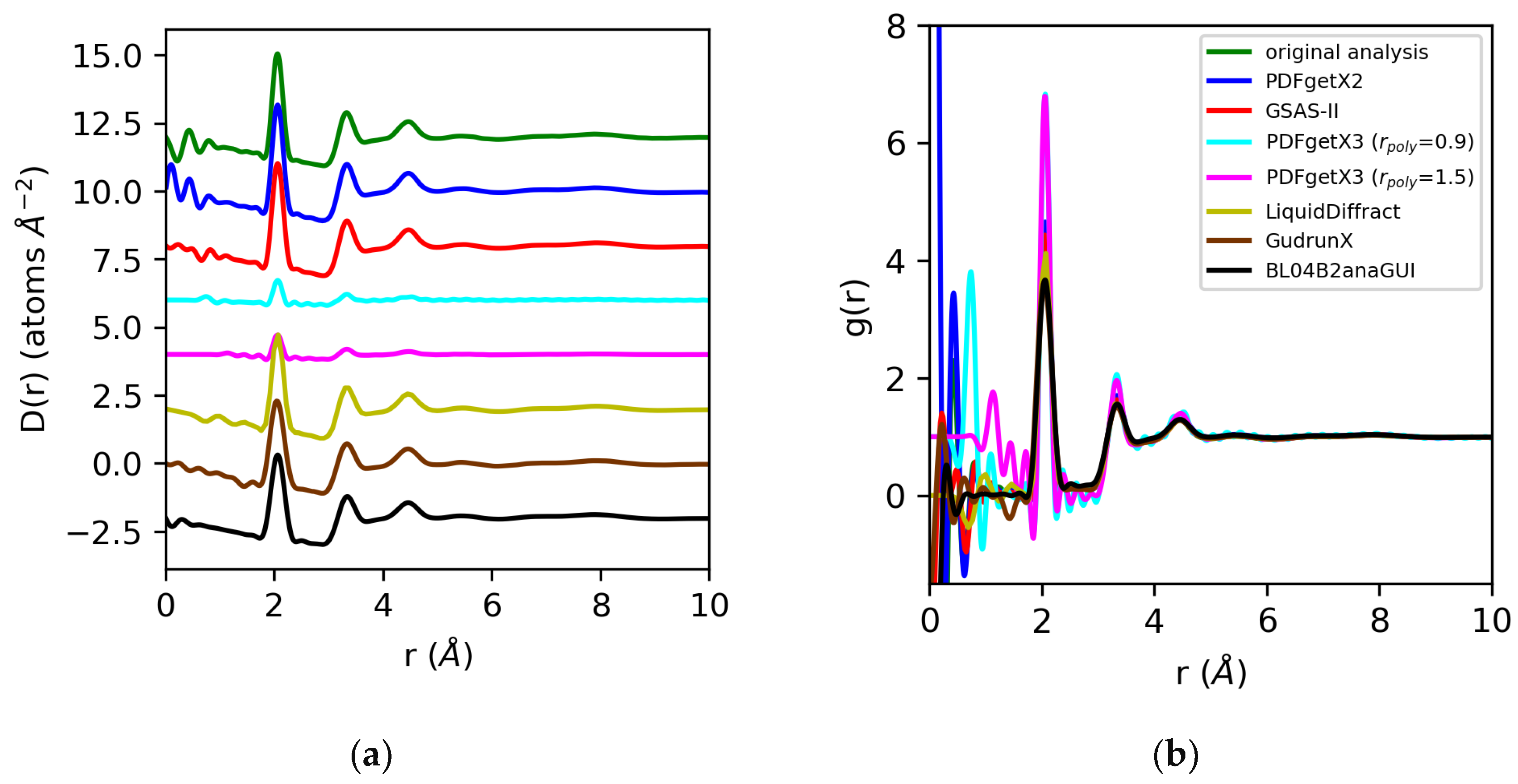
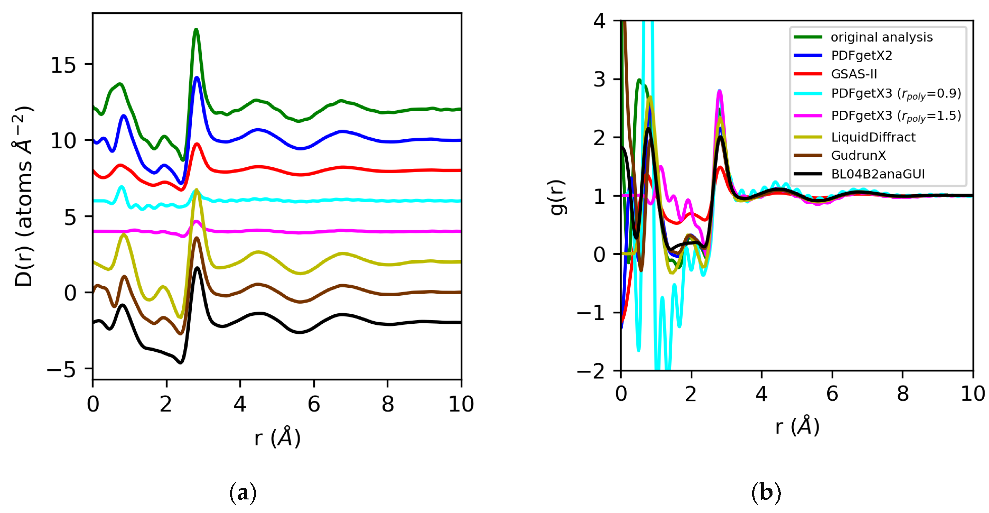
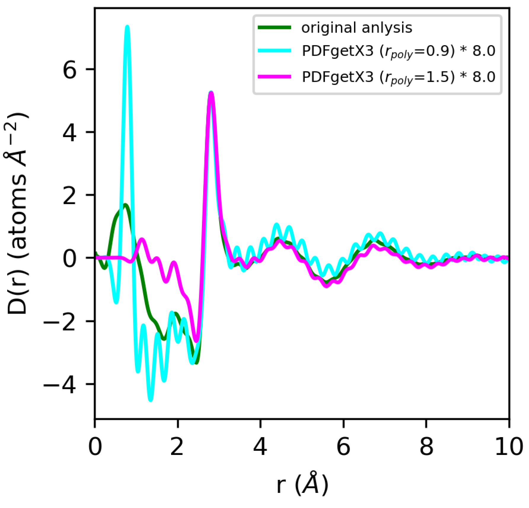
3.3. Comparison of Structure Factors and Pair Distribution Functions Obtained using Fast PDF Extraction Software Prior to Analyses

The structure factors for molten sulfur and water are shown in Figure 6 and Figure 7. An analysis of the X-ray total scattering data for sulfur in PDFgetX2, GSAS-II, LiquidDiffract, GudrunX, and BL042B2anaGUI yielded S(Q)s scaled within 5% of our prior analysis below Q = 5 Å−1, with increased deviation above Q = 15 Å−1. The direct rescaling of the peaks below Q = 5 Å−1 did not yield meaningful results for the structure factors obtained from PDFgetX3, as their limits as Q→0 diverged. This low Q divergence was significantly worsened when the order of the polynomial correction applied to the structure factor was increased. Comparison of [S(Q) − 1] revealed a factor of 5 difference in normalization between our prior analysis and that performed in PDFgetX3.
Analysis of the X-ray total scattering data for water, in contrast, resulted in much larger discrepancies in the normalization of the structure factors across the board [Figure 7]. All software packages tested in this review utilize atomic form factors, and do not have the option of including MAFFs. In prior analyses, the use of MAFFs in lieu of atomic form factors resulted in a 50% difference in the S(0) limit, and a visible 25–35% difference in the normalization of the low Q region (below Q = 3 Å−1) [Figure 2]. Additionally, hydrogen and oxygen are much weaker scatterers than sulfur, so effects such as background, dark current drift, fluorescence, and Compton scattering contribute to a significant fraction of the observed signal. Any discrepancies in correcting the data can lead to widely varying results in the overall scaling of the structure factors and pair distribution functions. The discrepancies in the normalization of the structure factors obtained using PDFgetX2, LiquidDiffract, GudrunX, and BL042B2anaGUI for peaks below Q = 3 Å−1 were −20%, −6%, −23%, and −18%, respectively, relative to our original analysis using atomic form factors. The direct rescaling of the peaks below either Q = 3 Å−1 or Q = 5 Å−1 did not yield meaningful results for the structure factors obtained using GSAS-II and PDFgetX3 due to the difference in the S(0) limit. A factor of 2.5 was found, and a 6.5 difference in the normalization of S(Q) − 1 using GSAS-II and PDFgetX3 (rpoly = 0.9 Å), respectively, was observed compared to that found in our original analysis. Increasing the order of the correction polynomial from 7 (rpoly = 0.9 Å) to 11 (rpoly = 1.5 Å) not only led to the greater divergence of S(Q) at low Q, but also resulted in an additional factor of 2.3 difference in the normalization of S(Q) − 1 [Figure 8].
The differential correlation functions, D(r), and pair distribution functions, g(r), for molten sulfur and water are shown in Figure 9 and Figure 10. The D(r)s obtained for sulfur extracted using PDFgetX2, GSAS-II, LiquidDiffract, GudrunX, and BL042B2anaGUI are qualitatively similar to those obtained in our prior analysis, and are scaled +4, −1%, −11%, −25%, and −24% relative to those results. The larger discrepancies in the normalization of D(r) compared to the structure factors are primarily due to the limited resolution of the PDF for LiquidDiffract, and the difference in the broadening of r for the PDFs obtained using GudrunX and BL042B2anaGUI. For the sulfur D(r)s extracted using PDFgetX3, the normalization is a factor of 4.4 lower than PDFgetX2 for both rpoly = 0.9 Å and rpoly = 1.5 Å. For all g(r)s except those from PDFgetX3, the atomic number densities were either explicitly set as equivalent to ρ = 0.0334 atoms/Å3 in the software (GSAS-II, LiquidDiffract, GudrunX), or assumed to be so during manual computation (PDFgetX2); therefore, any discrepancies in the normalization of D(r) were conserved. For PDFgetX3, assuming atomic number densities consistent with the low-r slope of D(r) resulted in an over-correction of the normalization, with the resulting g(r)s scaled roughly +50% above those obtained in our original analysis.
For water, we expect the significant errors we observe in the normalization of the structure factor to be propagated to the pair distribution functions derived from the Fourier transform. For PDFgetX2, GSAS-II, LiquidDiffract, GudrunX, and BL042B2anaGUI, the differences in normalization observed, at −22%, −66%, −10%, −32%, and −31%, respectively, relative to our original analysis using atomic form factors, are comparable to those observed in the structure factor. The D(r)s obtained for water in PDFgetX3 are mis-scaled by a factor of 8 for both rpoly = 0.9 Å and rpoly = 1.5 Å. This significantly differs from the scale factors required to renormalize the structure factor, which were 5 and 11.1, respectively [Figure 11]. Additionally, the correction polynomial yields a D(r) that is either extremely noisy, or completely smooths out the low-r O–H correlations. For all g(r)s except those from PDFgetX3, the atomic number densities were either explicitly set to ρ = 0.1003 atoms/Å3 in the software (GSAS-II, LiquidDiffract, GudrunX), or assumed to be so during manual computation (PDFgetX2); therefore, the discrepancy in the normalization of D(r) was conserved. For PDFgetX3, assuming atomic number densities consistent with the low-r slope of D(r) resulted in an over-correction of the normalization, much like molten sulfur, with the resulting g(r)s scaled roughly +13% above those obtained in our original analysis.
The coordination numbers for the first three sulfur–sulfur peaks calculated using Equation (6) are tabulated in Table 2. An atomic number density of ρ = 0.0334 atoms/Å3 was used for all calculations. The interatomic distances were obtained in our prior analysis were similar to those obtained using PDFgetX2, GSAS-II, LiquidDiffract, GudrunX, and BL04B2anaGUI. However, there was significant variability in the coordination numbers obtained from each program. The reduced real-space resolution for LiquidDiffract led to increasingly large discrepancies relative to our prior analyses, especially for the third shell. The subtle difference in the normalization of the structure factor in our simplified PDFgetX2 analysis compared with our prior, more rigorous, analyses is evident in the consistently larger coordination numbers obtained.

4. Conclusions

The advent of intense X-ray synchrotrons and their generation of vast amounts of scattering data have led to the deployment of rapid, highly automatable data analysis packages to keep pace with experiments. However, this has come at some cost in the case of studying highly disordered materials such as liquids. The results of our review highlight significant, and sometimes substantial, variations between the currently available total scattering software packages when applied to liquids. The lack of well-established correction procedures that can be employed to extract normalized S(Q)s can lead to serious issues when extracting coordination numbers from the pair distribution function, as illustrated by Figure 6, Figure 7 and Figure 8 and Table 2. In some cases, documentation of the theory behind the software computations is lacking, making it difficult to identify which steps are causing discrepancies in the output S(Q)s.
There has been rapid growth in the use of the PDF technique over the last decade, and many newcomers will not be familiar with the work of Wright some 30 years ago, which emphasized the importance of publishing the unphysical oscillations at low-r, below the first true peak in g(r). While these features may have no physical meaning, these oscillations are a strong indication of the level of systematic error in the PDF measurement. Any reviewer will not be able to judge the quality of the data if they are removed, especially if, as is common practice nowadays, the structure factor is not shown. Yet, to avoid introducing additional Fourier transform artifacts (ripples) into the PDF, some type of high-Q correction has to be applied to the data in order to enforce the condition S(Qmax) = 1. In addition, unless the data are perfect, the low-r unphysical region has to be removed in order to make comparisons with atomistic models that generate S(Q) and g(r) and are, by definition, zero in this region. Therein lies the challenge for experimentalists trying to model their data. For this reason, many researchers in the liquid and glass community opt to publish both the unphysical low-r oscillations in the raw Fourier transform, in addition to the model fits for which this region is naturally zero. Ideally, both the reduced S(Q) obtained using the appropriate corrections and the Fourier back-transform will also be published in reciprocal space.
Using the low-r unphysical region below the first true peak in the PDF to manipulate the data has previously been described as a “dubious” practice, and it has been stated that such data should be regarded with the “utmost suspicion” [33]. A more reasonable approach, for high-energy X-ray diffraction data at least, is to apply a small quadratic-type correction, since most corrections appear to have this general shape [2]. In large part, the purpose of this review has been to outline the best practices for using each software package currently available in order to make the appropriate corrections (and for the researcher to add those corrections that are missing) and so that the most accurate S(Q) and g(r) can be extracted. Unfortunately, this has not been possible for all software packages in the chosen examples of water and molten sulfur. Researchers should be aware of these issues when deciding how far to trust the data when interpreting liquid-state structures.

Supplementary Materials

The following supporting information can be downloaded at: https://www.mdpi.com/article/10.3390/qubs7020020/s1, Supporting Information on Data Collection and reduction, GudrunX Extended Discussion, and minimal code examples of extracting G(r) from GSAS-II, the IDL-based batch extraction of PDFs from PDFgetX2, and the python-IDL bridge-based batch extraction of PDFs from PDFgetX2. Reference [66] are cited in the Supplementary Materials.

Author Contributions

Conceptualization, L.C.G. and C.J.B.; methodology, L.C.G., S.K.W., S.K. and C.J.B.; validation, L.C.G., S.K.W., S.K. and C.J.B.; formal analysis, L.C.G., S.K.W., S.K. and C.J.B.; data curation, C.J.B.; writing—original draft preparation, L.C.G. and C.J.B.; writing—review and editing, L.C.G., S.K.W., S.K. and C.J.B.; visualization, L.C.G. and C.J.B. All authors have read and agreed to the published version of the manuscript.

Funding

This research was supported by the U.S. DOE Office of Science-Basic Energy Sciences, under Contract No. DE-AC02-06CH11357. This research was also supported by the JSPS KAKENHI Grants No. 20H05878 (to S.K.) and No. 20H05881 (to S.K.).

Data Availability Statement

Data is available on request.

Acknowledgments

This research used the resources of the Advanced Photon Source, a U.S. Department of Energy (DOE) Office of Science user facility at Argonne National Laboratory, and is based on research supported by the U.S. DOE Office of Science-Basic Energy Sciences, under Contract No. DE-AC02-06CH11357. This research was also supported by the JSPS KAKENHI Grants No. 20H05878 (to S.K.) and No. 20H05881 (to S.K.).

Conflicts of Interest

The authors declare no conflict of interest. The funders had no role in the design of the study; in the collection, analyses, or interpretation of data; in the writing of the manuscript; or in the decision to publish the results.

References

  1. Benmore, C.J. X-ray and neutron diffraction from glasses and liquids. In Reference Module in Chemistry, Molecular Sciences and Chemical Engineering; Elsevier: Amsterdam, The Netherlands, 2021. [Google Scholar]
  2. Skinner, L.B.; Benmore, C.J.; Parise, J.B. Area detector corrections for high quality synchrotron X-ray structure factor measurements. Nucl. Instrum. Methods Phys. Res. Sect. A Accel. Spectrometers Detect. Assoc. Equip. 2012, 662, 61–70. [Google Scholar] [CrossRef]
  3. Chupas, P.J.; Chapman, K.W.; Lee, P.L. Applications of an amorphous silicon-based area detector for high-resolution, high-sensitivity and fast time-resolved pair distribution function measurements. J. Appl. Crystallogr. 2007, 40, 463–470. [Google Scholar] [CrossRef]
  4. Hubbell, J.H.; Veigele, W.J.; Briggs, E.A.; Brown, R.T.; Cromer, D.T.; Howerton, R.J. Atomic form factors, incoherent scattering functions, and photon scattering cross sections. J. Phys. Chem. Ref. Data 1975, 4, 471–538. [Google Scholar] [CrossRef] [Green Version]
  5. Waasmaier, D.; Kirfel, A. New analytical scattering-factor functions for free atoms and ions. Acta Crystallogr. Sect. A Found. Crystallogr. 1995, 51, 416–431. [Google Scholar] [CrossRef]
  6. Paalman, H.H.; Pings, C.J. Numerical Evaluation of X-ray Absorption Factors for Cylindrical Samples and Annular Sample Cells. J. Appl. Phys. 1962, 33, 2635–2639. [Google Scholar] [CrossRef]
  7. Neuefeind, J.; Poulsen, H.F. Diffraction on disordered materials using “neutron-like” photons. Phys. Scr. 1995, 1995, 112–116. [Google Scholar] [CrossRef]
  8. Soper, A.K. Multiple scattering from an infinite plane slab. Nucl. Instrum. Methods Phys. Res. 1983, 212, 337–347. [Google Scholar] [CrossRef]
  9. Soper, A.K.; Egelstaff, P.A. Multiple scattering and attenuation of neutrons in concentric cylinders: I. Isotropic first scattering. Nucl. Instrum. Methods 1980, 178, 415–425. [Google Scholar] [CrossRef]
  10. Zaleski, J.; Wu, G.; Coppens, P. On the correction of reflection intensities recorded on imaging plates for incomplete absorption in the phosphor layer. J. Appl. Crystallogr. 1998, 31, 302–304. [Google Scholar] [CrossRef]
  11. Kohara, S.; Pusztai, L. Reverse Monte Carlo Simulations of Noncrystalline Solids. In Atomistic Simulations of Glasses: Fundamentals and Applications; Du, J., Cormack, A., Eds.; Wiley-American Ceramic Society: Westerville, OH, USA, 2022; pp. 60–88. [Google Scholar]
  12. Laaziri, K.; Kycia, S.; Roorda, S.; Chicoine, M.; Robertson, J.L.; Wang, J.; Moss, S.C. High-energy x-ray diffraction study of pure amorphous silicon. Phys. Rev. B 1999, 19, 13520–13533. [Google Scholar] [CrossRef] [Green Version]
  13. Klein, O.; Nishina, Y. Über die Streuung von Strahlung durch freie Elektronen nach der neuen relativistischen Quantendynamik von Dirac. Z. Für Phys. 1929, 52, 853–868. [Google Scholar] [CrossRef]
  14. Narten, A.H.; Levy, H.A. Liquid Water: Molecular Correlation Functions from X-ray Diffraction. J. Chem. Phys. 1971, 55, 2263–2269. [Google Scholar] [CrossRef]
  15. Narten, A.H. X-ray diffraction pattern and models of liquid benzene. J. Chem. Phys. 1977, 67, 2102–2108. [Google Scholar] [CrossRef]
  16. Narten, A.H.; Habenschuss, A. Hydrogen bonding in liquid methanol and ethanol determined by x-ray diffraction. J. Chem. Phys. 1984, 80, 3387–3391. [Google Scholar] [CrossRef]
  17. Soper, A.K. Joint structure refinement of x-ray and neutron diffraction data on disordered materials: Application to liquid water. J. Phys. Condens. Matter 2007, 19, 335206. [Google Scholar] [CrossRef]
  18. Skinner, L.B.; Huang, C.; Schlesinger, D.; Pettersson, L.G.M.; Nilsson, A.; Benmore, C.J. Benchmark oxygen-oxygen pair-distribution function of ambient water from x-ray diffraction measurements with a wide Q-range. J. Chem. Phys. 2013, 138, 074506. [Google Scholar] [CrossRef]
  19. Keen, D.A. A comparison of various commonly used correlation functions for describing total scattering. J. Appl. Crystallogr. 2001, 34, 172–177. [Google Scholar] [CrossRef]
  20. Hannon, A.C.; Howells, W.S.; Soper, A.K. ATLAS: A Suite of Programs for the Analysis of Time-of-flight Neutron Diffraction Data from Liquid and Amorphous Samples. Inst. Phys. Conf. Ser. 1990, 107, 193–211. [Google Scholar]
  21. Egelstaff, P.A. An Introduction to the Liquid State; Oxford University Press: Oxford, UK, 1994. [Google Scholar]
  22. Benmore, C.J.; Alderman, O.L.G.; Robinson, D.S.; Jennings, G.; Tamalonis, A.; Ilavsky, J.; Clark, E.; Soignard, E.; Yarger, J.; Weber, J. Extended range X-ray pair distribution functions. Nucl. Instrum. Methods Phys. Res. Sect. A Accel. Spectrometers Detect. Assoc. Equip. 2019, 955, 163318. [Google Scholar] [CrossRef]
  23. Winter, R.; Szornel, C.; Pilgrim, W.-C.; Howells, W.S.; Egelstaff, P.A.; Bodensteiner, T. The structural properties of liquid sulphur. J. Phys. Condens. Matter 1990, 2, 8427–8437. [Google Scholar] [CrossRef]
  24. Clark, G.N.I.; Hura, G.L.; Teixeira, J.; Soper, A.K.; Head-Gordon, T. Small-angle scattering and the structure of ambient liquid water. Proc. Natl. Acad. Sci. USA 2010, 107, 14003–14007. [Google Scholar] [CrossRef] [PubMed] [Green Version]
  25. Fine, R.A.; Millero, F.J. Compressibility of water as a function of temperature and pressure. J. Chem. Phys. 1973, 59, 5529–5536. [Google Scholar] [CrossRef]
  26. Fehér, F.; Hellwig, E. Beiträge zur Chemie des Schwefels, 45. Zur Kenntnis des flüssigen Schwefels. (Dichte, Ausdehnungskoeffizient und Kompressibilität). Z. Für Anorg. Und Allg. Chem. 1958, 294, 63–70. [Google Scholar] [CrossRef]
  27. Wright, A. Longer range order in single component network glasses? Phys. Chem. Glasses Eur. J. Glass Sci. Technol. Part B 2008, 49, 103–117. [Google Scholar]
  28. Soper, A.K.; Barney, E. On the use of modification functions when Fourier transforming total scattering data. J. Appl. Crystallogr. 2012, 45, 1314–1317. [Google Scholar] [CrossRef]
  29. Lorch, E. Neutron diffraction by germania, silica and radiation-damaged silica glasses. J. Phys. C Solid State Phys. 1969, 2, 229–237. [Google Scholar] [CrossRef]
  30. Krogh-Moe, J. A method for converting experimental X-ray intensities to an absolute scale. Acta Crystallogr. 1956, 9, 951–953. [Google Scholar] [CrossRef]
  31. Norman, N. The Fourier transform method for normalizing intensities. Acta Crystallogr. 1957, 10, 370–373. [Google Scholar] [CrossRef]
  32. Wright, A.C. Neutron scattering from vitreous silica. V. The structure of vitreous silica: What have we learned from 60 years of diffraction studies? J. Non-Cryst. Solids 1994, 179, 84–115. [Google Scholar] [CrossRef]
  33. Simmons, C.J.; El-Bayoumi, O.H. Experimental Techniques of Glass Science; Amer Ceramic Society: Columbus, OH, USA, 1993. [Google Scholar]
  34. Fischer, H.E.; Barnes, A.C.; Salmon, P.S. Neutron and x-ray diffraction studies of liquids and glasses. Rep. Prog. Phys. 2005, 69, 233–299. [Google Scholar] [CrossRef]
  35. Faber, T.E.; Ziman, J.M. A theory of the electrical properties of liquid metals. Philos. Mag. 1965, 11, 153–173. [Google Scholar] [CrossRef]
  36. Shannon, R.D. Revised effective ionic radii and systematic studies of interatomic distances in halides and chalcogenides. Acta Cryst. A 1976, 32, 751–766. [Google Scholar] [CrossRef]
  37. Shi, C. xINTERPDF: A graphical user interface for analyzing intermolecular pair distribution functions of organic compounds from X-ray total scattering data. J. Appl. Crystallogr. 2018, 51, 1498–1499. [Google Scholar] [CrossRef] [Green Version]
  38. McGreevy, R.L. Reverse Monte Carlo modelling. J. Phys. Condens. Matter 2001, 13, R877–R913. [Google Scholar] [CrossRef]
  39. McGreevy, R.L.; Pusztai, L. Reverse Monte Carlo Simulation: A New Technique for the Determination of Disordered Structures. Mol. Simul. 1988, 1, 359–367. [Google Scholar] [CrossRef]
  40. Soper, A.K. Empirical potential Monte Carlo simulation of fluid structure. Chem. Phys. 1996, 202, 295–306. [Google Scholar] [CrossRef]
  41. Soper, A.K. Tests of the empirical potential structure refinement method and a new method of application to neutron diffraction data on water. Mol. Phys. 2001, 99, 1503–1516. [Google Scholar] [CrossRef]
  42. Coelho, A. TOPAS and TOPAS-Academic: An optimization program integrating computer algebra and crystallographic objects written in C++. J. Appl. Crystallogr. 2018, 51, 210–218. [Google Scholar] [CrossRef] [Green Version]
  43. Coelho, A.A.; Chater, P.A.; Kern, A. Fast synthesis and refinement of the atomic pair distribution function. J. Appl. Crystallogr. 2015, 48, 869–875. [Google Scholar] [CrossRef]
  44. Farrow, C.L.; Juhas, P.; Liu, J.W.; Bryndin, D.; Božin, E.S.; Bloch, J.; Proffen, T.; Billinge, S.J.L. PDFfit2 and PDFgui: Computer programs for studying nanostructure in crystals. J. Phys. Condens. Matter 2007, 19, 335219. [Google Scholar] [CrossRef] [Green Version]
  45. Skinner, L.B.; Benmore, C.J.; Weber, J.K.R.; Du, J.; Neuefeind, J.; Tumber, S.K.; Parise, J.B. Low Cation Coordination in Oxide Melts. Phys. Rev. Lett. 2014, 112, 157801. [Google Scholar] [CrossRef] [PubMed]
  46. Soper, A.K. Network structure and concentration fluctuations in a series of elemental, binary, and tertiary liquids and glasses. J. Phys. Condens. Matter 2010, 22, 404210. [Google Scholar] [CrossRef] [PubMed]
  47. Hammersley, A.P.; Svensson, S.O.; Hanfland, M.; Fitch, A.N.; Hausermann, D. Two-dimensional detector software: From real detector to idealised image or two-theta scan. High Press. Res. 1996, 14, 235–248. [Google Scholar] [CrossRef]
  48. Qiu, X.; Thompson, J.W.; Billinge, S.J.L. PDFgetX2: A GUI-driven program to obtain the pair distribution function from X-ray powder diffraction data. J. Appl. Crystallogr. 2004, 37, 678. [Google Scholar] [CrossRef] [Green Version]
  49. Toby, B.H.; Von Dreele, R.B. GSAS-II: The genesis of a modern open-source all purpose crystallography software package. J. Appl. Crystallogr. 2013, 46, 544–549. [Google Scholar] [CrossRef]
  50. Juhás, P.; Davis, T.; Farrow, C.L.; Billinge, S.J.L. PDFgetX3: A rapid and highly automatable program for processing powder diffraction data into total scattering pair distribution functions. J. Appl. Crystallogr. 2013, 46, 560–566. [Google Scholar] [CrossRef] [Green Version]
  51. Heinen, B.J.; Drewitt, J.W.E. LiquidDiffract: Software for liquid total scattering analysis. Phys. Chem. Miner. 2022, 49, 9. [Google Scholar] [CrossRef]
  52. Soper, A.K.; Barney, E.R. Extracting the pair distribution function from white-beam X-ray total scattering data. J. Appl. Crystallogr. 2011, 44, 714–726. [Google Scholar] [CrossRef]
  53. Kohara, S.; Itou, M.; Suzuya, K.; Inamura, Y.; Sakurai, Y.; Ohishi, Y.; Takata, M. Structural studies of disordered materials using high-energy x-ray diffraction from ambient to extreme conditions. J. Phys. Condens. Matter 2007, 19, 506101. [Google Scholar] [CrossRef]
  54. Egami, T.; Billinge, S.J.L. Underneath the Bragg Peaks: Structural Analysis of Complex Materials; Elsevier: Amsterdam, The Netherlands, 2003. [Google Scholar]
  55. Ruland, W. The separation of coherent and incoherent Compton X-ray scattering. Br. J. Appl. Phys. 1964, 15, 1301–1307. [Google Scholar] [CrossRef]
  56. Yang, X.; Juhas, P.; Farrow, C.L.; Billinge, S.J. xPDFsuite: An end-to-end software solution for high throughput pair distribution function transformation, visualization and analysis. arXiv 2014, arXiv:1402.3163. [Google Scholar]
  57. Eggert, J.H.; Weck, G.; Loubeyre, P.; Mezouar, M. Quantitative structure factor and density measurements of high-pressure fluids in diamond anvil cells by x-ray diffraction: Argon and water. Phys. Rev. B 2002, 65, 174105. [Google Scholar] [CrossRef]
  58. Soper, A.K. Inelasticity corrections for time-of-flight and fixed wavelength neutron diffraction experiments. Mol. Phys. 2009, 107, 1667–1684. [Google Scholar] [CrossRef] [Green Version]
  59. Igor Pro, Version 8; WaveMetrics, Inc.: Lake Oswego, OR, USA. Available online: http://www.wavemetrics.com (accessed on 1 May 2023).
  60. Hart, R.T.; Benmore, C.J.; Neuefeind, J.; Kohara, S.; Tomberli, B.; Egelstaff, P.A. Temperature Dependence of Isotopic Quantum Effects in Water. Phys. Rev. Lett. 2005, 94, 047801. [Google Scholar] [CrossRef] [Green Version]
  61. Ohara, K.; Onodera, Y.; Murakami, M.; Kohara, S. Structure of disordered materials under ambient to extreme conditions revealed by synchrotron x-ray diffraction techniques at SPring-8—Recent instrumentation and synergic collaboration with modelling and topological analyses. J. Phys. Condens. Matter 2021, 33, 383001. [Google Scholar] [CrossRef]
  62. Sasaki, S. KEK Report 83-22, 88-14; National Laboratory for High Energy Physics: Tsukuba, Japan, 1984; Volume 1989. [Google Scholar]
  63. Cromer, D.T.; Mann, J.B. Compton Scattering Factors for Spherically Symmetric Free Atoms. J. Chem. Phys. 1967, 47, 1892–1893. [Google Scholar] [CrossRef] [Green Version]
  64. Waseda, Y. The Structure of Non-Crystalline Materials: Liguids and Amorphous Solids; Mcgraw-Hill Publishing: New York, NY, USA, 1980. [Google Scholar]
  65. Press, W. Numerical Recipes in Fortran 77: The Art of Scientific Computing; Cambridge University Press: New York, NY, USA, 1992. [Google Scholar]
  66. Soper, A.K. GudrunN and GudrunX: Programs for Correcting Raw Neutron and X-ray Diffraction Data to Differential Scattering Cross Section; Science & Technology Facilities Council: Swindon, UK, 2010. [Google Scholar]
Figure 1. Normalized electron intensity I(Q) comprising the sum of the X-ray form factors (self-scattering) and Compton scattering for molten sulfur (a) and water (b). Both atomic and modified atomic form factors are shown for water.
Qubs 07 00020 g001
Figure 2. The raw X-ray structure factors for molten sulfur (a) and water (b) obtained using atomic form factors and MAFF’s for water. The corresponding S(0) values based on isothermal compressibilities (symbols) and extrapolation to Qmin (dotted line) are also shown.
Qubs 07 00020 g002
Figure 3. The differential correlation functions, D(r), for (a) molten sulfur using a direct Fourier transform (thin line) and a Lorch function applied (thick line). (b) Water analyzed using atomic and modified form factors with the intramolecular structure removed and the Lorch function applied.
Qubs 07 00020 g003
Figure 4. The measured X-ray structure factors for (a) molten sulfur (using atomic form factors) and (b) water (obtained using modified atomic form factors), compared to the Fourier back-transform (FBT) where g(r < 1.9 Å) = 0 (sulfur) and g(r < 0.55 Å) = 0 (water).
Qubs 07 00020 g004
Figure 5. The measured X-ray structure factors for molten sulfur and water and EPSR 3D structural models (a), and the running coordination numbers for S–S, O–H and O–O extracted from the EPSR models (b).
Qubs 07 00020 g005
Figure 6. Structure factors S(Q) (a) and Q[S(Q) − 1] (b) for molten sulfur extracted from X-ray total scattering data from original analysis (green) vs. those obtained via PDFgetX2 (blue), GSAS-II (red), PDFgetX3 with rpoly = 0.9 (cyan) and rpoly = 1.5 (magenta), LiquidDiffract (gold), GudrunX (brown), and BL04B2anaGUI (black).
Qubs 07 00020 g006
Figure 7. Structure factors S(Q) (a) and Q[S(Q) − 1] (b) for water extracted from X-ray total scattering data from original analysis using atomic form factors (green) vs. those obtained using PDFgetx2 (blue), GSAS-II (red), PDFgetX3 with rpoly = 0.9 Å (cyan) and rpoly = 1.5 Å (magenta), LiquidDiffract (gold), GudrunX (brown), and BL042B2anaGUI (black).
Qubs 07 00020 g007
Figure 8. Comparison of structure factors S(Q) (a) and Q[S(Q) − 1] (b) for water extracted using PDFgetX3 with rpoly = 0.9 Å (cyan) and rpoly = 1.5 Å (magenta) vs. our original analysis (green). Quantities from PDFgetX3 have been manually renormalized for ease of comparison with our original analysis.
Qubs 07 00020 g008
Figure 9. Differential correlation distribution functions (a) and pair distribution functions (b) for molten sulfur extracted from X-ray total scattering data using original analysis (green) vs. those obtained using PDFgetx2 (blue), GSAS-II (red), PDFgetX3 with rpoly = 0.9 Å (cyan) and rpoly = 1.5 Å (magenta), LiquidDiffract (gold), GudrunX (brown), and BL042B2anaGUI (black). Lorch modification functions were applied in all cases except PDFgetX3.
Qubs 07 00020 g009
Figure 10. Differential correlation distribution functions (a) and pair distribution functions (b) for water extracted from X-ray total scattering data using original analysis with atomic form factors (green) vs. those obtained using PDFgetX2 (blue), GSAS-II (red), PDFgetX3 with rpoly = 0.9 Å (cyan) and rpoly = 1.5 Å (magenta), LiquidDiffract (gold), GudrunX (brown), and BL042B2anaGUI (black). Lorch modification functions were applied in all cases except PDFgetX3.
Qubs 07 00020 g010
Figure 11. Comparison of differential correlation functions for water extracted using PDFgetX3 with rpoly = 0.9 Å (cyan) and rpoly = 1.5 Å (magenta) vs. our original analysis (green). Quantities from PDFgetX3 have been manually renormalized for ease of comparison with our original analysis.
Qubs 07 00020 g011
Table 2. S–S distances and coordination numbers (for peaks 1, 2 and 3) obtained in original analysis with atomic form factors vs. those obtained using fast PDF extraction in various software suites. Errors of up to 5% are typical for coordination numbers derived from these analyses [2,18].
ProgramrSS(1)
(Å)
nSS(1)
(1.80–2.30 Å)
rSS(2)
(Å)
nSS(2)
(3.00–3.60 Å)
rSS(3)
(Å)
nSS(3)
(4.20–4.74 Å)
Original analysis2.051.883.323.134.465.54
PDFgetX22.062.013.333.244.465.75
GSAS-II2.051.93.343.064.475.52
LiquidDiffract2.071.93.33.134.455.98
GudrunX2.041.923.323.064.445.55
BL04B2anaGUI2.061.913.333.204.465.64
Disclaimer/Publisher’s Note: The statements, opinions and data contained in all publications are solely those of the individual author(s) and contributor(s) and not of MDPI and/or the editor(s). MDPI and/or the editor(s) disclaim responsibility for any injury to people or property resulting from any ideas, methods, instructions or products referred to in the content.

