Article

A New Water Film Depth Prediction Model for Pavement Surface Drainage

1
College of Civil Engineering, Nanjing Forestry University, Nanjing 210037, China
2
Logistics Department, Nanjing Sport Institute, Nanjing 210014, China
3
Shandong Lu Qiao Group Co., Ltd., Jinan 250000, China
*
Authors to whom correspondence should be addressed.
Infrastructures 2024, 9(3), 36; https://doi.org/10.3390/infrastructures9030036
Submission received: 19 December 2023 / Revised: 21 January 2024 / Accepted: 20 February 2024 / Published: 21 February 2024
(This article belongs to the Section Infrastructures Materials and Constructions)

Abstract

:
The prediction of the water film depth (WFD) on the road surface can help with road skid resistance research and reduce the risk associated with driving on rainy days. At present, there are many empirical and analytical models based on drainage length, slope, rainfall intensity and other parameters. Considering the influence of road surface runoff and starting from the Reynolds number formula of road surface water flow, a new road surface WFD calculation formula that considers the movement state of laminar water flow is derived. The results show that the changing trends of various parameters in the prediction model (drainage length, rainfall intensity, road slope) affecting WFD are consistent with those of the existing model. It is also found that the initial water film depth, initial speed of rainwater, and rainfall angle have little impact on WFD. The predicted value of the model has a suitable matching degree compared with the classical empirical model, which provides a new approach to the prediction of road water film depth.

1. Introduction

When rainfall occurs, the frequency of traffic accidents significantly increases. Rain makes road surfaces slippery, reducing vehicle traction and often causing accidents like skidding, overturning, or rear-end collisions [1,2,3,4]. Hence, the WFD on the road becomes a critical indicator because the formation of a water film can cause a partial loss of contact between vehicles and the road surface, resulting in hydroplaning. This issue becomes more severe when the water film depth exceeds a certain limit, leading to pronounced hydroplaning. Previous research [5,6,7,8] has shown a close correlation between rainfall volume, road surface characteristics, and water film depth (WFD). For instance, rainfall directly affects the amount of water on the road [9,10], while the horizontal and vertical slopes affect the road drainage distance. Additionally, road texture and material properties play a crucial role in providing pathways for rainwater flow and absorbing some of the rainfall. Road drainage and skid resistance on rainy days comprise a very complex issue. The depth of the water film on the road surface, the driving speed, and the contact between the tires and the road surface are all important factors that affect driving safety on rainy days [11,12,13]. In recent years, relevant scholars have considered the influence of roadway slope and pavement texture to predict the spatiotemporal water film depth under dynamic rainfall profiles, predicting the slip speed of vehicles traveling in different lanes based on tire–water–road interaction. Therefore, the accumulation of water on road surfaces during rainy conditions, forming a water film, diminishes road traction, posing significant safety hazards. Absolutely, minimizing this potential risk is paramount in road construction. Therefore, it is essential to delve into the factors influencing road surface water film and accurately predict water film depth during rainy conditions.
There are various methods for estimating water film depth (WFD), including the following. Empirical Models: These models rely on known data and empirical rules. They often consider factors like rainfall volume, road surface characteristics, and slopes, but are limited to specific environmental data. For instance, in 1968, Ross et al. [14] conducted experiments and introduced the well-known RRL model. Then, in 1971, Gallaway et al. [15] carried out experiments under windless conditions, enhancing the water film depth prediction model by incorporating pavement construction depth T based on the RRL model. In 1982, Wambold et al. [16] observed data through experiments with a drainage length of 11 m. They defined the water film depth above the pavement structure depth as the surface water film depth and used multiple linear regression to determine coefficients, obtaining the prediction formula for surface water film depth. John Anderson [17] conducted experiments in 1995 to analyze water depth on typical road surfaces, and the factors influencing it. Using a regression method, he derived a well-known empirical formula in the UK. Generally speaking, the most widely used models include the Ross and Russam model [14], the Gallaway model [15], the PAVDRN model, the New Zealand modified equation [18,19] and other models. These models take into account factors such as rainfall intensity, pavement slope, pavement texture, etc. The M. Kane model [12] relates to comprehensive models that consider more road surface and weather conditions; the relevant disclosures are shown in Table 1. The researchers conducted modifications on the model parameters and artificial rainfall experiments to improve the accuracy of the model. Although the main models used in different countries and regions vary slightly, empirical models are commonly used in predicting WFD. The study found that the empirical PAVDRN [20,21] and Gallaway models are more effective in WFD calculations, and are especially suitable for rigid pavements. However, these models work under steady-state flow conditions and do not adequately consider the effects of different rainfall intensities. It should be noted that there are still certain limitations and problems that need to be solved, such as the development of methods for determining coefficient values and confronting difficulties in extending the model beyond experimental procedures.
Empirical regression models are derived based on empirical data and are suitable for specific parameter ranges, but are limited by road surface characteristics and environmental changes [22]. Researchers turned to analytical methods, using hydraulic equations and fluid mechanics principles, such as Manning’s formula, Chezy’s formula, and the two-dimensional shallow water equation [23], to derive more accurate predictive models. However, these classic methods face limitations in considering road flow characteristics, slope changes, and rainfall timing. Researchers have proposed a series of new models, including artificial neural network models that consider factors such as pavement width and changes in rainfall intensity [24], models based on two-dimensional shallow water equations, and models that consider water flow conditions and pavement structure depth [25]. These models comprehensively consider more factors that affect WFD, improving the applicability and accuracy of the model. Among them, the analytical WFD model [26] more comprehensively simulates the changes in WFD by dynamically considering rainfall intensity, pavement geometry, texture characteristics, and other factors. In recent years, there have been models that consider drainage issues, models based on theoretical hydraulic analysis, and models that consider drainage capacity under different rainfall intensities, etc. [27]. These models improve the theoretical prediction ability of WFD by comprehensively considering the geometric characteristics, drainage capacity and other factors of actual roads.
Table 1. Summary of prediction models of pavement WFD.
SourceEquation Form
Ross and Russam (RRL) [14] WFD = 0.017 × ( L I ) 0.47 i 0.2
Gallaway [15] WFD = 0.01485 × ( MTD 0.11 L 0.43 I 0.59 i 0.42 ) MTD
Wambold [16] WFD = 0.005979 × ( MTD 0.11 I 0.59 i 0.42 ) MTD  (L = 11)
John Anderson [17] WFD = 0.015 × ( L I ) 0.5 i 0.5
New Zealand modified [18] WFD = 0.003264 × ( L 0.316 I 0.2712 i 0.3 ) MTD
Empirical PAVDRN [20] WFD = 0.00073 × ( L 0.519 I 0.562 MTD 0.125 i 0.364 ) MTD
J. Luo [28] WFD = 0.068 × L 0.32 I 0.41 MTD 1.17 i 0.31
M. Kane [12] h t + V h x + h V x = i f e V t + V V x + g h x = g ( S 0 S f ) + ( i f e ) V h
Two-dimensional shallow water-governing equation [23] U t + F ( U ) x + h G ( U ) y = Q U = h u h v h , F = u h u 2 h + 0.5 g h 2 u v h G = v h u v h v 2 h + 0.5 g h 2 , Q = q r g h S 0 , x g h S f , x g h S 0 , y g h S f , y
W. Luo [26] WFD = ( Q 0 Q s n Q p Q d a c ) / S
K. Wang [27] WFD = I 7 / 12 ( 0.3164 v 0.25 8 g i ) 1 / 3 x 7 / 12
While predictive models for water film depth (WFD)—namely, empirical models, statistical methods, and complex system modeling—offer relatively accurate predictions, those reliant on empirical data or equations show distinct limitations [29,30,31]. These limitations encompass the oversight of factors such as pavement texture and permeability, restricted applicability linked to localized empirical data, the inadequacy of fixed rainfall intensity values in capturing diverse precipitation environments, and constraints in accounting for various road surface types in WFD computations [26,32,33,34]. These collective constraints hinder a comprehensive and precise prediction of water film depth across diverse conditions and regions. Although mathematical models facilitate the theoretical analysis of water film depth, the intricacies of slope flow during rainfall pose challenges in solving differential equations. Simplification often leads to substantial deviations from real-world scenarios. This study focuses on analyzing and exploring the theoretical computation of water film over short pathways. It adopts initial water film depth instead of construction depth and incorporates rainfall drop velocity as a parameter. The research establishes a theoretical analytical model for road surface water film depth, grounded in constant total flow continuity and constant total flow momentum equations. By solving these differential equations, the study conducts comparative analyses through trial calculations, aiming to comprehend the influence patterns of key factors on water film depth.

2. Intervening Factors on Pavement WFD

Under rainfall conditions, several factors affect pavement water film depth, illustrated in Figure 1. Key parameters include the length of surface drainage (L), rainfall intensity (I), pavement slope (i or the angle α between the pavement and the horizontal line, i = sinα ≈ tanα), initial depth of the water film (h0), initial velocity of raindrops (u0), and rainfall angle (β).
Domestic and international scholars have explored methods such as multiple linear regression and range analysis to assess the significance of each parameter in influencing pavement water film depth under rainfall conditions [6,29]. Significance tests have been employed to rank the degree of influence of each factor on water film depth.

2.1. Drainage Length (L)

In China, various highway grades typically feature a single lane width of 3.75 m. For multi-lane roads, like a unidirectional four-lane expressway, the total width for lanes in one direction can reach 15 m. This implies that, during rainfall, the runoff’s drainage length on a unidirectional road could extend up to 15 m. On extensive slopes, this increased drainage length might prompt distinctions between laminar and turbulent flow along the slope, necessitating differentiation in theoretical analyses.
Fluid dynamics recognizes two primary flow states: laminar and turbulent flow. Laminar flow occurs when fluid particles move in a parallel fashion without mixing, and are characterized by smooth paths. Turbulent flow, however, involves chaotic paths where fluid particles mix, collide, and create disorder. These distinct states not only vary in particle trajectories but also exhibit entirely different internal flow structures, including velocity distribution and pressure characteristics. Consequently, their head loss and diffusion patterns differ, resulting in entirely distinct head losses along the flow. Hydraulic studies extensively investigate these associated head losses.
When evaluating hydraulic aspects of runoff on sloping surfaces, understanding the disparities between laminar and turbulent flows holds significant importance. Theoretically establishing the critical point where these flow states transition is pivotal, enabling distinct discussions on runoff characteristics within each flow state range. During the theoretical analysis of these critical transition conditions, it becomes essential to examine the criterion distinguishing laminar and turbulent flows—the critical Reynolds number. In industry standards, for a circular pipe, the industry has experimentally determined R e k = 2320 and R e k = 12,000–50,000. Due to the instability of the upper critical Reynolds number, engineers typically use the lower critical Reynolds number in practical applications. Therefore, for a circular pipe:
R e = v d υ
When R e < R e k = 2320, the flow state is laminar; otherwise, it is turbulent.
The Reynolds number can be understood as the ratio between the inertial forces and the viscous forces in a fluid flow.
Inertia force m a = ρ V d v d t , and its dimension is ρ L 3 L T 2 ; viscous force T = μ d u d y , and its dimension is μ L 2 1 T . The ratio of inertial force and viscous force can be expressed as
v i s c o u s   f o r c e i n e r t i a   f o r c e = ρ L 4 T 2 μ L 2 T 1 = L 2 T ν
The above formula is the dimensional composition of the Reynolds number, where L / T is the characteristic flow velocity, L is the characteristic length, and υ is the kinematic viscosity coefficient.
The above criteria are for liquid flow in circular tubes. For other flow boundaries, they also include laminar flow and turbulent flow, as well as corresponding Reynolds numbers and critical Reynolds numbers. The characteristic length of an open channel can be characterized by its hydraulic radius.
Hydraulic radius refers to the ratio of the water-passing cross-sectional area A to the wetted perimeter χ, represented by R, and has the length dimension. Therefore, for a pipe flow with diameter d, the hydraulic radius is
R = A χ = π d 2 / 4 π d = d 4
Then, the corresponding Reynolds number and critical Reynolds number are
( R e ) R = v R υ
( R e k ) R = v k R υ = v k d / 4 υ 2320 4 = 580
The critical Reynolds number relative to an open channel is roughly 500.
In this article, the characteristic length used when examining the Reynolds number is the depth h of the water film on the road surface; that is, the Reynolds number with slope runoff is:
R e = v R υ = v h υ
In analyzing road runoff, determining the hydraulic gradient J is crucial. It is essential to discern whether the flow pattern of slope runoff is laminar or turbulent during the analysis. Differentiating between the runoff characteristics of these flow patterns is imperative as they exhibit distinct behaviors. Hence, examining the Reynolds number of slope runoff becomes necessary to identify the critical threshold that distinguishes these flow states. This critical position allows for a separate discussion of the runoff characteristics on either side of this threshold.
The formula for calculating the Reynolds number of slope runoff ( R e = v R υ = v h υ ) highlights two key parameters for examination on the right side of the equation: v and h. Here, v denotes the runoff velocity at a specific point along the slope, while h represents the slope’s gradient at that same point.
The viscosity of the flowing liquid, denoted as υ in the formula, determines the depth of the water film. It is found that at 15 °C, the dynamic viscosity (υ) of water is 1.139 × 10⁻⁶ m2/s. When evaluating v and h, directly determining the relationship between the Reynolds number of slope runoff and 500 from these two quantities becomes challenging. On one hand, the water film depth (h) on the slope, which this article aims to calculate, remains an unknown quantity. Additionally, the runoff velocity (v) is difficult to examine in isolation. On the other hand, the Reynolds number (Re) is currently a variable dependent on two variables, making direct analysis more difficult.
Hence, finding a simpler method to distinguish the flow pattern of slope runoff becomes necessary. As per the research model outlined in this article, the relationship between rainfall recharge and cross-section runoff flow is established as:
q = v h = I L cos α
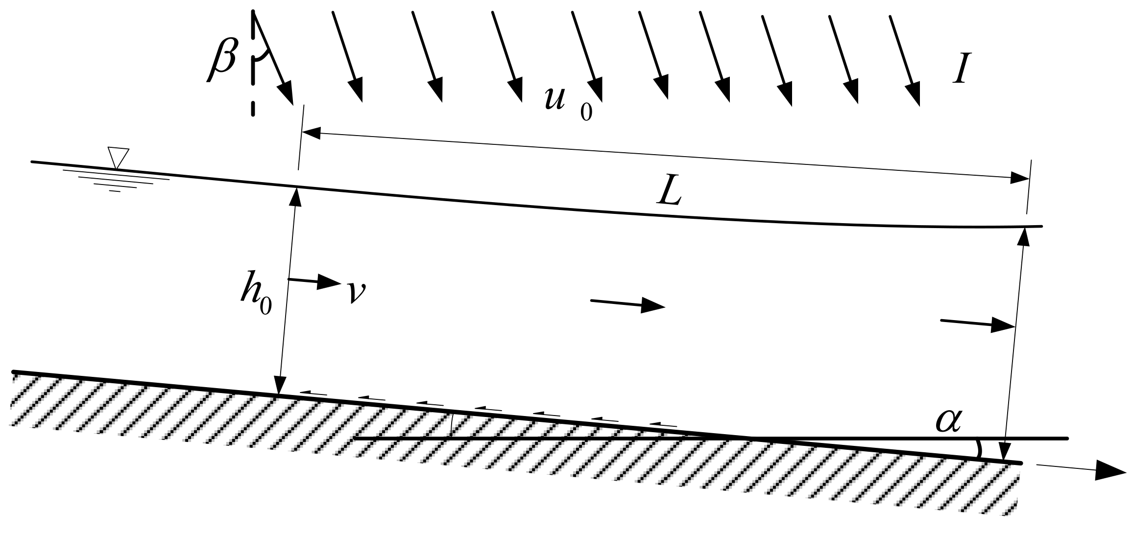
In the formula, q represents the flow value of a certain section along the runoff direction; I represents rainfall intensity; s represents the distance between the section and the center line of the road surface, that is, the drainage length of slope runoff; α represents the slope angle of the slope surface and the slope of the road i = sinα ≈ tanα.
In this way, the Reynolds number of slope runoff can be expressed as:
R e = v R υ = v h υ = I L cos α υ
In the formula above, the Reynolds number’s most pertinent variables are rainfall intensity (I), drainage length (L), and cosα associated with the slope. Among these factors, for a specific slope under consideration, rainfall intensity and cosα remain constant. This simplifies the Reynolds number of slope runoff into a singular variable that solely varies with drainage length, significantly minimizing the complexity of the discussion regarding the magnitude of the Reynolds number.
Moreover, the determination of the transition between laminar and turbulent flow hinges upon the Reynolds number. This critical point is situated at a specific location along the slope in the runoff direction, represented by a particular drainage length “L”. By equating the equation with a constant and comparing it to 500, a critical value of “L”, referred to as “critical s”, can be derived. This value precisely indicates the critical juncture between laminar and turbulent flow in surface runoff. Such an approach enables a clear-cut discussion of surface runoff on both sides of the critical value, “critical L”.
R e = s × 0.05 × 10 3 m / s 1.139 × 10 6 m / s 2 = 500
The Reynolds number calculation formula, R e = I s cos α υ , shows that at a fixed drainage length, the determined Reynolds number varies with different rainfall intensities (I) and slope gradients (i). When considering a rainfall intensity of I = 3.0 mm/min = 0.05 × 10⁻³ m/s and a slope gradient of i = 5%, R e = s × 0.05 × 10 3 m / s 1.139 × 10 6 m / s 2 . When Re is 500, s equals 8.78 m, which indicates that the critical s is 8.78 m.
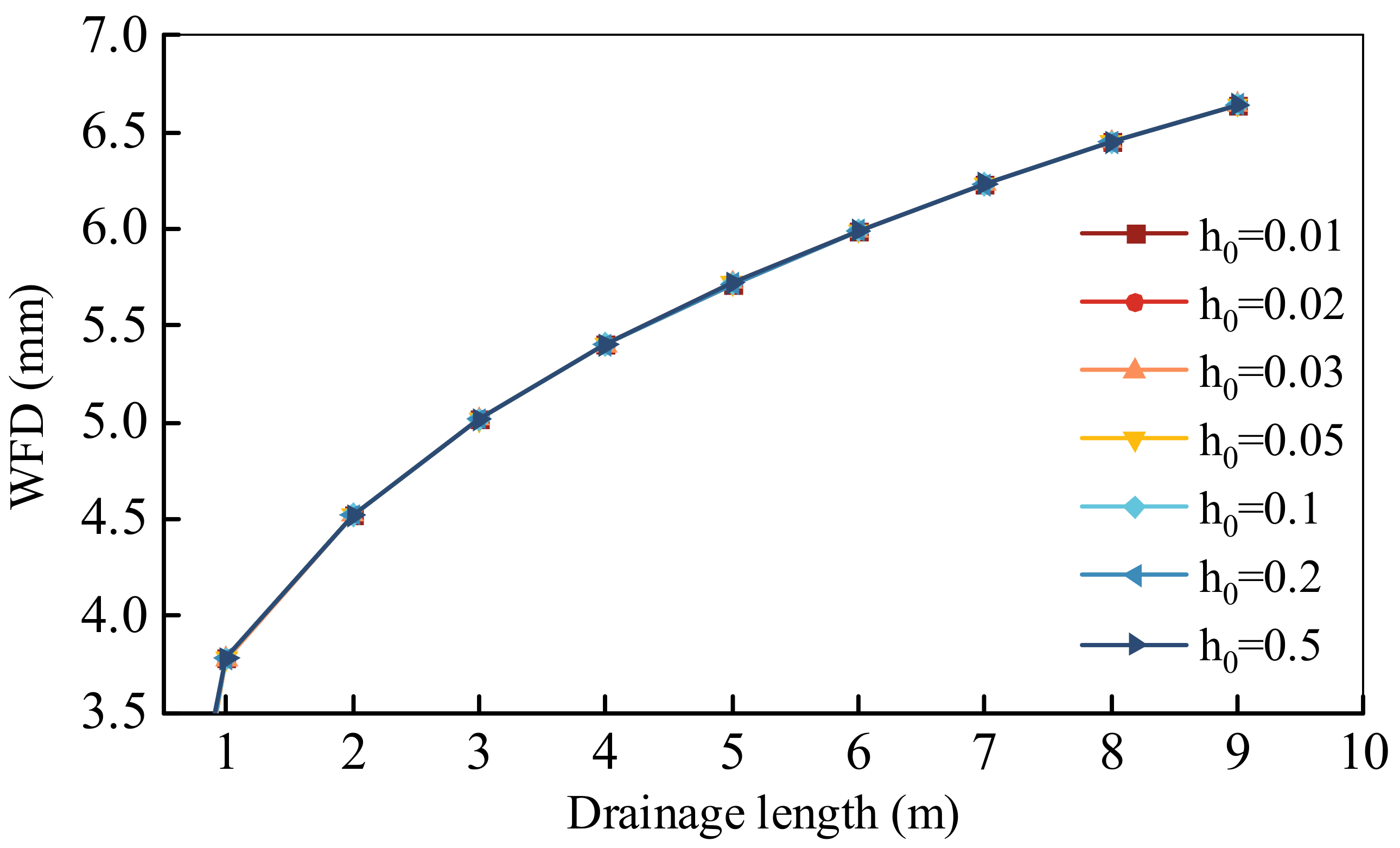
To streamline the discussion, this study concentrates solely on investigating laminar flow conditions while examining surface runoff characteristics. The analysis of turbulent flow scenarios remains a subject for future studies. For simplicity, and based on the previously calculated critical value of L, an approximation assumes that within a drainage length of 9 m, surface runoff predominantly maintains laminar flow. Consequently, this research delves into scrutinizing surface runoff within a drainage length of 9 m for the calculation of road surface water film depths during rainfall conditions. This research scope serves adequately for typical single-lane, two-way roads, and these simplified research findings possess reference value even for shorter slope lengths. The drainage length, denoted as “L”, ranges from 0 to 9 m, encompassing values at 0 m, 1 m, 2 m, 3 m, 4 m, 5 m, 6 m, 7 m, 8 m, and 9 m, totaling ten values. At s = 0, it signifies the initial depth of the water film on the road surface, referred to as h0.

2.2. Rainfall Intensity (I)

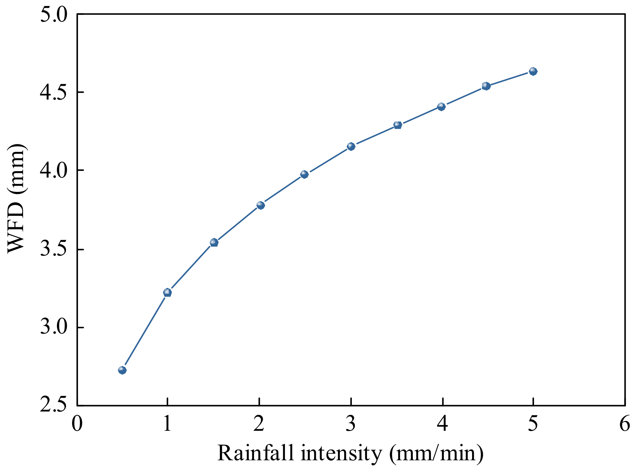
Rainfall intensity, denoted as I, stands as a crucial factor impacting water film depth on road surfaces during rainy conditions. Empirical evidence underscores that different levels of rainfall intensity wield a substantial influence on the water film’s depth over road surfaces. When maintaining a consistent drainage length, road surface gradient, and raindrop velocity, there is a clear trend indicating escalated water film depth with increased rainfall intensity. This observation aligns with historical experimental data, emphasizing the pronounced impact of rainfall intensity, especially during heavy downpours or stormy weather, on road surface water film depth. Hence, delving into the effects of diverse rainfall intensities on road surface water film depth assumes significance, contributing to a comprehensive comprehension of water film behavior during rainfall. This paper recognizes the significant influence of rainfall intensity among the factors affecting road surface water film depth. It seeks to explore the correlation between varying levels of rainfall intensity and road surface water film depth.
To study the relationship between road surface water film depth and rainfall intensity, the primary concern is determining the magnitude of rainfall intensity under different rainy conditions. Regarding the selection of rainfall intensity values in the design calculation process, the “Highway Drainage Design Specification” (JTG/T D33—2012) provides explicit regulations, as follows.
Using standard rainfall intensity contour maps and relevant conversion coefficients, calculate the rainfall intensity according to the equation q = cpctq5,10, where q5,10 represents the standard rainfall intensity (mm/min) for a 5-year return period and 10 min duration; cp signifies the return period conversion coefficient, which is the ratio of design return period rainfall intensity qp to the standard return period rainfall intensity q5; ct stands for the duration conversion coefficient, which is the ratio of rainfall intensity qt for duration t to rainfall intensity q10 for a 10 min duration
By consulting the “China 5-year return period 10-min rainfall intensity contour map”, it can be observed that the 5-year return period 10 min rainfall intensity, q5,10, in the southeastern coastal regions of China generally ranges from 2.0 mm/min to 2.5 mm/min, with the maximum national value of q5,10 being 3.0. Upon converting the standard rainfall intensity to values corresponding to durations below 10 min according to the table above, the converted rainfall intensity surpasses 3.0 mm/min, reaching approximately 4 to 5 mm/min.
Considering the aforementioned factors, this paper outlines the range of rainfall intensity utilized in the calculations, set between 0.5 to 5 mm/min. Specifically focusing on examining the correlation between road surface water film depth and rainfall intensity, the analysis involves comparing various rainfall intensities: 0.5 mm/min, 1.0 mm/min, 1.5 mm/min, 2.0 mm/min, 2.5 mm/min, 3.0 mm/min, 3.5 mm/min, 4.0 mm/min, 4.5 mm/min, and 5.0 mm/min. These ten values were utilized to juxtapose the curves of rainfall intensity versus water film depth, intending to establish the general trend of road surface water film depth (h) concerning the variations in rainfall intensity (I).

2.3. Road Surface Gradient (i)

In road surface runoff, the road gradient is another factor affecting the water film depth during rainfall. While studies indicate that the influence of the gradient (i) on road surface water film depth ranks relatively low among rainfall factors, its impact becomes substantial in cases of substantial gradient variations. Consequently, various research reports on road surface water film depth under rainfall consider the effect of road surface gradient (i). The gradient encompasses the longitudinal slope along the road’s profile and the cross-slope across the road, including combinations of both longitudinal and cross-slopes. Under rainfall, the actual water film depth on the road surface results from the combined effects of these diverse gradient scenarios.
The typical cross-slope of road surfaces, denoted as i, commonly ranges between 1.0% and 3.5%. For wider road surfaces aiming to enhance drainage efficiency, this percentage can be appropriately increased to approximately 4.0% or even higher. Considering these factors comprehensively, and aiming to qualitatively explore the impact of road surface gradient on water film depth concerning rainfall intensity, the gradient range (i) was set between 1.0% and 6.0%.
In particular, for a specific analysis centered on the effect of increased road surface gradient while assuming consistency in the other three factors, gradient values (i) were set as 0.5%, 1.0%, 1.5%, 2.0%, 2.5%, 3.0%, 3.5%, 4.0%, 4.5%, 5.0%, 5.5%, and 6.0%. These twelve values were employed to compute the corresponding water film depths for each gradient, establishing a quantitative relationship between water film depth and road surface gradient.

2.4. Initial Water Film Depth (h0)

In the early stages of rainfall, especially during low intensity rain, rainwater initially occupies the gaps on the road surface, essentially filling the voids within the structural depth. At this juncture, the road surface does not exhibit standing water, yet a water film persists, indicating an extremely minimal initial water film depth on the road surface.
To precisely depict the depth of rainwater, establishing a stable surface runoff during rainfall, this study introduces the concept of “initial water film depth”, denoted as h0. The scope for the initial water film depth is notably narrow. Hence, this research undertakes a comparison and computation of the initial water film depth across values of 10 μm, 20 μm, 30 μm, 50 μm, 100 μm, and 200 μm.

2.5. Physical Parameters of Raindrops

The physical attributes of raindrops during rainfall play a significant role in shaping the water film on road surfaces. These key parameters typically encompass the angle between raindrops influenced by wind and the vertical line (referred to as the rainfall angle, β in Figure 1), along with the terminal velocity of the raindrops (u0 in Figure 1).
It is commonly understood that as atmospheric water vapor cools and condenses, it transforms into minute liquid or solid water droplets, occasionally developing into ice crystals. These minuscule droplets or crystals merge and accumulate over time, gradually growing in size and weight, forming larger water droplets. When these droplets’ gravitational force surpasses the upward atmospheric movement, they descend, initiating rainfall. The terminal velocity (u0) of raindrops signifies the immediate speed at which a raindrop reaches the ground following its descent.
The descent of raindrops involves a process marked by variable acceleration. As a raindrop descends, both the forces influencing it and its speed undergo continuous changes. The forces acting on a falling raindrop typically include gravity, atmospheric buoyancy, and air resistance, the latter fluctuating as the raindrop’s speed changes during its descent. Air resistance is approximated to be proportional to the square of the falling speed for larger raindrops, while for smaller ones, it is considered proportional to the falling speed itself.
Research indicates that the terminal velocity of raindrops increases with their size. Raindrops with a diameter of 6 mm (commonly maintaining a diameter of less than 6 mm during descent) can achieve a terminal velocity of around 10 m/s upon reaching the ground. This substantial speed carries significant momentum upon impact, highlighting the importance of considering raindrop terminal velocity in discussions regarding surface runoff processes.
Numerous studies, both domestically and internationally, have delved into the terminal velocity of falling raindrops. Theoretical formulas for the terminal velocity (u0) have been derived through theoretical analysis, yet actual measured data remain limited. Notably, related research [35,36] has conducted dedicated experiments exploring raindrop terminal velocity, compiling the statistical data presented in Table 2. These experiments utilized pulse induction and recorded droplet fall durations via computerized means. By adjusting the height difference of droplet falls, approximate terminal velocity values were derived. The methodology employed in the experiment was comprehensive, carrying significant importance for research focused on rainfall phenomena.
In this study regarding the calculation of road surface water film depth under rainfall conditions, consideration was given to the impact of raindrop terminal velocity (u0). In several existing reports [24,27,37] on the calculation of road surface water film depth, both domestically and internationally, there has been little discussion about the influence of raindrop terminal velocity on road surface water film depth. However, based on the aforementioned analysis, during heavy rainfall, raindrop terminal velocities can reach speeds of nearly 10 m/s, resulting in a substantial impact on the ground. Regarding the value of β, previous research has indicated that under typical wind conditions (up to level 6 wind), the maximum angle of raindrop descent does not exceed 50° [38,39,40,41]. In the study of road surface runoff, considering the relatively shallow and lightweight nature of the water film on the road surface, the impact caused by a higher momentum due to raindrop terminal velocity cannot be disregarded when acting on the water film on the road surface, as it significantly influences the entire road surface runoff.

3. Methodology

3.1. Theoretical Basis

3.1.1. Conservation of Mass Equation

The discussed overland flow in this paper falls under the category of steady flow. In establishing equations relating road surface water film depth (h) to various factors, one crucial equation is the continuity equation for the incremental liquid flow along the slope’s direction. This equation holds significant importance in modeling the relationship between rainfall supply and parameters such as section runoff flow. It greatly simplifies the fundamental differential equation for road surface water film depth and facilitates the solution of the differential equation.
The continuity equation refers to an equation that reflects the conservation of liquid mass, demonstrating the conservation of mass in the flow of liquid during its movement. The continuity equation for steady flow comprises the continuity equation of elemental flow and the total flow continuity equation. These equations, from both microscopic and macroscopic perspectives, reveal the relationship regarding the conservation of mass in the flow of liquid.
The area and velocity of the elemental flow at the water passage section are denoted as dA1, dA2, u1, and u2 respectively. The area and velocity of the total flow at the water passage section are denoted as A1, A2, v1, and v2 respectively, as shown in Figure 2. For the elemental flow section, there is no interaction between the fluid’s side and the outer liquid flow, and there are no voids within the elemental flow.
So, for compressible fluids, there exists ρ1v1A1 = ρ2v2A2, and for incompressible fluids, there exists v1A1 = v2A2.
The continuity equation derived earlier does not encompass any conditions related to force or time. Instead, it is a dynamic equation reflecting the conservation of flow between two sections along the fluid’s path and establishing the connection between section area and velocity. It is applicable to ideal and real fluids, steady and unsteady flows, as well as uniform and non-uniform flows. In the study of overland flow characteristics, this paper also employs a continuity equation to illustrate changes in flow across overland surfaces.

3.1.2. The Momentum Equation for Steady Total Flow

The fundamental principle applied in this paper to study overland flow involves deriving an equation relating road surface water film depth to rainfall intensity, the drainage length of overland flow, the slope gradient, and the raindrop terminal velocity—it is the momentum equation for steady flow. By establishing the force acting on one side of the momentum equation and the relationship between the mass and velocity of the fluid on the other side, it essentially encompasses all factors influencing road surface WFD.
Therefore, utilizing the momentum equation for runoff to establish the relationship between road surface water film depth and various influencing factors, analyzing and solving the momentum equation to obtain the relationship between road surface water film depth and each factor, and calculating the theoretical values of road surface water film depth under various rainfall and slope conditions constitute the fundamental methodology and approach of this study.
The core theoretical approach of this study relies on the principles of the fluid momentum equation and continuity equation from hydraulics and hydrology. Thus, it can be said that the investigation of road surface water film depth under rainfall conditions in this paper is theoretically deduced based on hydraulic and hydrological principles, marking its distinction and innovation compared to other related research.
The momentum equation of a fluid is the mathematical expression of the principle of conservation of momentum in fluid motion. This, along with the continuity equation and energy equation, constitutes the “three fundamental laws” of hydraulics. The momentum equation in fluid motion illustrates the relationship between changes in the momentum of a fluid and the external forces acting on the fluid as it moves.
One side of the equation represents the resultant force acting on the fluid in the direction under study, while the other side expresses the change in momentum of the fluid in that direction. Thus, the parameters related to fluid movement encompassed in the momentum equation are quite comprehensive, and this advantage is precisely utilized in this paper.
In theoretical mechanics, the momentum theorem for a system of particles defines that the rate of change of momentum of the system of particles per unit time equals the total force acting on the system, as per Newton’s second law, expressed as
F = M a = M d v d t = d d t M v = d P d t
where F represents the resultant external force acting on the system of particles, M represents the mass of the particle system, v represents the velocity of the particle, P represents the momentum of the particle system, and t represents time.
Based on this theoretical foundation, it is possible to establish a momentum equation for fluid motion.
First, we establish a liquid flow model as shown in Figure 3, which shows any isolator in the constant flow total flow. We assume that the areas of the water-passing sections of the total flow section at time t0 are A1 and A2, respectively, and the average liquid flow velocities on the two sections are v1 and v2, respectively. After Δt time, the original water passes sections 1-1 and 1-2. The water body moves to sections 1′-1′ and 2′-2′ along the direction of liquid flow. It is important to highlight that in the context of studying the liquid flow as an incompressible fluid, the mass and flow rate within the interval between 1′-1′ and 2-2 can be assumed to remain constant. Consequently, when comparing the liquid flow volume at time t0 with that at time t0 + Δt, it can be inferred that the momentum of the fluid within the 1′-1′ and 2-2 intervals remains consistent across these two time points. According to the fact that the total flow volume of the liquid flow at a certain fixed moment is equal to the sum of the momentum of each component of the total flow, the momentum before and after Δt can be expressed as:
P 1 2 = P 1 1 + P 1 2
P 1 2 = P 1 2 + P 2 2
where P 1 2 represents the total momentum of the flow of the whole isolator at time t0. P 1 1 represents the momentum of the liquid flow between section 1-1 and section 1′-1′ at time t0, which can be expressed as P 1 1 = A 1 ρ u u d A Δ t , where ρ is the density of the liquid flow. P 1 2 represents the momentum of the liquid flow on the isolator at time B between section 1′-1′ and section 2-2. p 1 2 represents the total momentum of the whole isolator flow at time t0 + Δt. P 1 2 represents the momentum of the liquid flow on the isolator at time t0 + Δt between section 1′-1′ and section 2-2. p 2 2 represents the momentum of the liquid flow between section 2-2 and section 2 at time t0 + Δt, and its value can be expressed as:
P 2 2 = A 2 ρ u u d A Δ t .
In this way, it can all be obtained from the following formula:
F = d P d t = lim Δ t 0 P 1 2 P 1 2 Δ t = lim Δ t 0 P 1 2 + P 2 2 P 1 1 P 1 2 Δ t = lim Δ t 0 P 2 2 P 1 1 Δ t = lim Δ t 0 A 2 ρ u u d A Δ t A 2 ρ u u d A Δ t Δ t = A 2 ρ u u d A A 1 ρ u u d A
There are also formulas for hydraulics:
A u 2 d A = α v 2 A = α v Q
Therefore, the resultant force on the liquid flow can be expressed as:
F = A 2 ρ u u d A A 1 ρ u u d A = α 2 ρ v 2 v 2 A 2 α 1 ρ v 1 v 1 A 1
where α 1 and α 2 represent the kinetic energy correction coefficients of sections 1-1 and 2-2 sections. v 1 and v 2 represent the average velocity at the cross sections 1-1 and 2-2 of the liquid flow isolator, respectively.
In general, α 1 α 2 1 and satisfy v 1 A 1 = v 2 A 2 = Q at the same time, so we can infer:
F = ρ Q ( v 2 v 1 )
When analyzing the force characteristics of the liquid flow isolator, the value of F can also be expressed as follows:
F = F 1 + F 2 + G + R
where F 1 and F 2 represent the total water pressure at section 1-1 and section 2-2 of the liquid flow isolator, respectively. G represents the weight of the liquid flow isolator. R represents the constrained resistance of the pipe wall during the flow of the total flow isolator.
Generally speaking, the momentum equation of the liquid flow is expressed separately on the three axes of the Cartesian coordinate system:
F x = ρ Q ( α 2 v 2 x α 1 v 1 x ) F y = ρ Q ( α 2 v 2 y α 1 v 1 y ) F z = ρ Q ( α 2 v 2 z α 1 v 1 z )
The above formula is the scalar form of the liquid flow equation. v1x, v1y, v1z, v2x, v2y and v2z in the formula are the components of v1 and v2 on the three coordinate axes, respectively. When their directions are consistent with the coordinate axes, they take positive values, otherwise they take negative values. ∑Fx, ∑Fy and ∑Fz are the projections of the resultant force on the three coordinate axes, respectively. When their direction is consistent with the direction of the coordinate axis, it takes a positive value; otherwise, it takes a negative value.
When the momentum equation of liquid flow is used to analyze the motion characteristics of fluid, the appropriate liquid flow isolator and coordinate axis should be selected to make clear the direction of each external force. When using the formula F = F 1 + F 2 + G + R to calculate the resultant force on the part of the liquid flow isolator, the direction of R can be assumed in advance. After the final result is calculated, if the value is positive, the actual direction of R is consistent with the direction assumed in advance, and vice versa. In general, in engineering practice, the momentum equation of liquid flow is combined with the continuity equation of liquid flow and the energy equation of fluid, which can comprehensively reflect the flow properties of liquid flow.
When deriving the momentum equation in the fluid motion of a steady flow, it is assumed that the liquid flow is an incompressible liquid, so that the velocity and mass of the fluid remain constant between the 1′-1′ cross-section and the 2-2 section; that is, the momentum of the liquid flow in these sections remains constant, which is helpful in simplifying the derivation process of the momentum equation. This assumption limits the application of the momentum equation of liquid flow. However, in the slope runoff studied in this paper, it can be considered that the water body of the runoff part is incompressible; that is, for the slope flow, the momentum equation can be established to describe the relationship between the motion parameters.

3.2. New WFD Model

On the basis of theory and basic assumptions, considering the role of raindrops, the theoretical analysis and research model of the water film depth on road surfaces under rainfall can be obtained. As shown in Figure 4, the s-axis parallel to the slope direction and the axis perpendicular to the slope direction are used as two orthogonal axes. Among them, the coordinate origin of the L axis and the h axis is on the centerline of the road surface. Take a point L on the L axis along the slope direction, and assume that the water film depth of the point is h and the runoff velocity is v. In order to study the dynamic characteristics of slope runoff, take the micro increment ds along the L axis direction, and assume that the water film depth increment of the L + dL point relative to the s point is dh and the velocity increment is dv; that is, the water film depth is h + dh, and the runoff velocity is v + dv.
For impervious pavements, the loss of rainwater through infiltration when it flows along the road slope is not considered in the formulation of the research model. Initially, it is essential to establish both the continuity equation for slope runoff and the momentum equation governing the liquid flow within the aforementioned model.
The basic idea of establishing the continuity equation is that the rain water flow per unit time through the water section at L + dL consists of two parts, namely, the rain water flow per unit time through the s section and the rainfall replenishment flow formed by rainfall in the ds section of the isolator per unit time, and the variation of the flow between the two water sections of the isolator is the rainfall recharge on this section. The rain water flow per unit time flowing through the L section is the rainfall recharge flow from the center line of the road to the L.
Consider the unit width:
v h + I d L cos α = v + d v h + d v
d ( v h ) = d q = I cos α d L
q = v h = I L cos α
The basic idea of establishing the momentum equation of slope runoff is to first analyze the resultant force of the water body in the isolation section in the flow process, and then analyze the flow and velocity of the isolation section based on the formula F = ρ Q v 2 v 1 . The force of the water body in the isolation section includes the water pressure along the L-axis on the cross-section at the L-point, the water pressure in the opposite L-axis direction on the water-crossing section at L + dL, the gravity of the water body in the isolation section and the shear stress in the opposite L-axis direction at the point of contact with the slope. If the variation in the momentum of the isolator on the right side of the equation includes the momentum of the flow on the water cross-section at point L, the momentum of the flow on the water cross-section at L + dL, and the momentum of the rainfall recharge part accepted by the isolation section, then
F s = 1 2 ρ g h 2 1 2 ρ g ( h + d h ) 2 τ 0 d L + ρ g h d L sin α                 = ρ ( q + d q ) ( v + d v ) ρ q v ρ d q u 0 sin ( α + β )
where v represents the average flow velocity of the cross-section at point s; h represents the water film depth of the cross-section at point L; I represents rainfall intensity; q represents the rainwater flow flowing through the section at point L per unit time; dv represents the variable at point L + dL relative to the average flow velocity of the cross-section at point s. The average flow velocity of the cross-section at point L + dL is v + dv; dh represents the variable of the water film depth of the road surface at point L + dL relative to the cross-section at point s. The water film depth at point L + dL is h + dh; α represents the angle between the road slope and the horizontal plane; ∑Fs represents the resultant force along the s-axis direction on the flow of the isolation body from s to L + dL; ρ represents the density of rainwater, which is used in the calculation as 1.0 × 10³ kg/m3; τ0 represents the shear stress of the water body in the isolation section at the point of contact with the slope surface, τ0 = ρgRJ = ρghJ, and R is the hydraulic radius of the fluid. In this article, the hydraulic radius of runoff is equal to the depth of the road water film, that is, R = h, while J is the hydraulic radius. When Re < 500, the slope runoff is in laminar flow, and the hydraulic slope J = (3υ/gh3)v; u0 represents the final speed of raindrops when they hit the road; β represents the angle between the raindrop’s fall and the vertical direction.
We can simplify the above formula and get
ρ g h d h ρ g h J d L + ρ g h i d L = ρ d [ q v q u 0 sin ( α + β ) ] = ρ d [ v 2 h v h u 0 sin ( α + β ) ]
Dividing both sides by ρghds at the same time, we get
d h d L J + i = 1 g h d d L [ v 2 h v h u 0 sin ( α + β ) ] = 1 g h d d L [ q v q u 0 sin ( α + β ) ] = 1 g h d d L [ I 2 L 2 cos 2 α 1 h I L cos α u 0 sin ( α + β ) ]
By sorting out the above equation, we can get the basic differential equation.
d d L q v q u 0 sin α + β 1 2 g h 2 = g h i J
This paper only studies a situation wherein the slope runoff is in laminar flow, that is, the Reynolds number Re < 500. We can bring J = 3 υ g h 3 v = 3 υ g h 3 I L cos α h into the formula to get
d h d L 3 υ I L cos α g h 4 + i = 1 g h 2 I 2 L cos 2 α h 2 I 2 L 2 h 2 d h d L I L cos α u 0 sin α + β
By multiplying h4 on both sides, the differential equation of water film depth h to the drainage length s of runoff can be obtained.
h 4 + I 2 cos 2 α g h L d h d L + i h 4 + I cos α u 0 sin α + β g h 3 2 I 2 cos 2 α g L h 2 3 υ I cos α g L = 0
The equation contains only h, s, I, i, u0, α, β and other parameters. This is also the differential equation to be studied and solved directly, which will be discussed later.
It is assumed that the a 1 = I 2 cos 2 α g , a 2 = I cos α u 0 sin α + β g , a 3 = 2 I 2 cos 2 α g and a 4 = 3 υ I cos α g relations can be reduced to
( h 4 + a 1 h L 2 ) d h d L + i h 4 + a 2 h 3 a 3 L h 2 a 4 L = 0
This equation is the main basis for the following study of the relationship between pavement water film depth and various influencing factors. By solving this equation, the relationship between pavement water film depth and drainage length can be discussed quantitatively. The relationship between water film depth, rainfall intensity and slope can be qualitatively analyzed. In order to draw conclusions for this paper, the problem to be solved now is the differential Equation (29), and the solution method is discussed below.
Generally, for some typical ordinary differential equations, their general expressions can be obtained and the arbitrary constants in the expressions can be determined by the initial conditions. However, the range of ordinary differential equations with this solution is relatively small, and is usually limited to linear ordinary differential equations and a small number of linear coefficient equations. In general, for the more extensive and nonlinear general differential equations, there is usually no elementary function formula solution; for this kind of equation, we can only find its approximate numerical solution. In general, the calculation accuracy of the Longkuta method is high, so this method is usually used to yield the approximate numerical solution.

4. Results and Discussion

4.1. Parametric Analysis

4.1.1. Relationship between WFD and Drainage Length of Road Surface

In the previous article, a general statement has been made on the method of studying and discussing the relationship between the water film depth h and the drainage length s of runoff under the condition of rainfall. As mentioned above, when discussing the relationship between pavement water film depth, rainfall intensity and slope, the distribution of pavement water film depth h along the drainage length s is obtained by using different rainfall intensity I values or slope I values. Therefore, this paper will yield more calculation results under various rainfall conditions and slope conditions to reflect the relationship between the water film depth h of the road surface and the drainage length s of the runoff. Therefore, this paper only takes a group of values of rainfall intensity I, slope I and raindrop velocity u0, calculates the water film depth of each point along the drainage direction, and draws the conclusion that the water film depth of the road surface varies with the drainage length.
In this section, in order to study the relationship between water film depth and drainage length, a group of values related to rainfall conditions and slope conditions includes rainfall intensity I = 3.0 mm/min = 0.00005 m/s, slope i = 5%, and the final velocity of raindrops u0 = 10 m/s. For rain water dynamic viscosity, we set v = 1.139. The above parameters are brought in (26), and the differential equation containing only the water film depth of the road surface and the drainage length of the runoff is obtained. The h values of each point within 9 m along the L direction are calculated. What is worth explaining here is that, theoretically, the water film depth h of the road surface at the drainage length swarm 0 should be 0, but the result of this calculation is that the water film depth values of all points along the L direction are 0, which obviously does not accord with the actual situation. For this reason, a small amount is taken for the water film depth h of the road surface at the initial condition swarm 0. Through the comparison of different small quantities, it is found that when the initial condition h is small enough, the value of h has no effect on the calculation results. In this paper, the initial condition h0 is taken as = 0.000001, and the water film depth of each point is calculated, as shown in Figure 5.
It can be seen from the diagram that when the rainfall intensity, slope and raindrop velocity are constant, the water film depth of the road surface increases nonlinearly with the increase in the drainage length of runoff. Near the centerline of the road cross-section, the water film depth h increases rapidly with the increase in the drainage length, and the growth rate tends to be flat when the drainage length is longer. Of course, this result is based on the premise of rainfall intensity = 3.0 mm/min = 0.00005 m/s, slope = 5%, and the final velocity of raindrops u0 = 10 m/s. The representativeness of this conclusion needs to be discussed in a variety of cases.
Later, this paper will study the effects of different rainfall conditions and slope conditions on pavement water film depth, so as to obtain the relationship between pavement water film depth and runoff drainage length; that is, under the condition of rainfall, when the rainfall intensity, slope and raindrop velocity are constant, the pavement water film depth increases linearly with the increase in drainage length. And the growth rate gradually slows down with the increase in the distance from the road’s centerline.

4.1.2. Relationship between WFD and Rainfall Intensity on Road Surface

As mentioned earlier, because the differential Equation (29) is the differential relation between the pavement water film depth h and the drainage length s, it is difficult to discuss the relationship between the pavement water film depth h and the rainfall intensity I directly using this equation. Therefore, according to the method of discussing the relationship between water film depth and drainage length in the previous section, the slope I and raindrop velocity u0 are constant when using several gradually increasing rainfall intensity values I (29). We solve the value of the water film depth on the road surface at each point along the s direction in each case, and then take out the value of the water film depth in each case for a specific drainage length s. Next we establish a one-to-one corresponding relationship with the I value of rainfall intensity in various cases.
First of all, for the road slope I and the final velocity of raindrops u0, we set i 0.05% and u0 = 10 m/s in the calculation, and I and u0 are regarded as constant in the calculation of each rainfall intensity. Of course, when other values are used for I and u0, the final conclusion about the relationship between road surface water film depth and rainfall intensity is consistent, but for the same rainfall intensity, there is a difference in the calculated value of road surface water film depth. For the value of rainfall intensity, this paper uses a total of 10 values 0.5~5.0 mm/min, with an interval of 0.5. It is worth pointing out that, in order to unify the parameter data unit when solving the differential equation, the unit of rainfall intensity is uniformly converted to m/s when it is brought in. Here, when finding the approximate numerical solution of the differential equation under each rainfall intensity, when the initial condition is also taken as 0, h0 = 0.000001. The numerical solution of the relationship between the water film depth and the drainage length is obtained, and then the water film depth h value at a fixed drainage length in each case is obtained, thus the corresponding relationship between the water film depth and the rainfall intensity is established under the condition that the drainage length, slope and raindrop velocity are the same. It should be noted that, for this particular drainage length, this paper uniformly use 5 m, because when the drainage length of the runoff reaches 5 m, the flow is relatively stable, and when other values are used, the same conclusion can be obtained. The curve of the relationship between the depth of water film and rainfall intensity is shown in Figure 6.
The relationship between pavement water film depth and rainfall intensity can be obtained from Figure 6. Under the condition that the drainage length of runoff, road slope and the final velocity of raindrops are the same, the pavement water film depth increases with the increase in rainfall intensity, showing a gradual increasing trend. Moreover, when the rainfall intensity I is small, the water film depth h increases greatly with its growth; when it reaches 3.0 mm/min, the change rate of the water film depth slows down with the increase in I, in the basic form of linear growth. It can be inferred from the picture that the water film depth of the road surface at the same point will increase greatly because of the increase in rainfall intensity, which is also an important reason why traffic accidents are more common in heavy rain or rainstorm weather than in light rainfall weather. Therefore, the influence of rainfall intensity on the depth of road water film cannot be ignored.

4.1.3. Relationship between WFD and Road Slope

When studying the relationship between pavement water film depth and pavement slope, the method used is the same as the method used in the previous section to discuss the relationship between water film depth and rainfall intensity, on the premise that other influencing factors are consistent. By taking different values into the slope value I in the differential Equation (29), the water film depth values of various points on the road surface under various conditions are solved. We then extract the water film depth value obtained from a specific drainage length s according to different slope I values, establish a one-to-one corresponding relationship with the I value, and then draw each point in the hmuri coordinate system and synthesize the change relation curve. The general relationship between water film depth and rainfall intensity is thus obtained. This method avoids the difficulty met in directly discussing the water film depth h and the slope I by using Equation (29) of the differential relation between h and s, which makes the study simple.
Before solving the water film depth of the pavement under different slope values, the values of the relevant parameters should be explained. For the values of the two characteristic parameters, rainfall intensity I and raindrop velocity u0, which reflect rainfall conditions, this section takes the values of 3.0 mm/min and 10 m/s. As mentioned in the previous section, the unit of rainfall intensity should be converted into m/s when it is brought into the calculation so that the parameter units can be unified. Of course, if we use other rainfall conditions here, we derive the same conclusion, but there are some differences in the specific calculation results. For the slope to be discussed, this section uses a total of 12 values ranging 0.5–6.0% with intervals of 0.5 to calculate the water film depth of the road surface in each case. For the specific length of runoff drainage to be studied, this section also addresses 5 m. Of course, when discussing other drainage lengths, it is possible to draw the same conclusion as this section. The curve of the relationship between water film depth and slope is shown in Figure 7.
From Figure 7, we can draw a conclusion about the relationship between pavement water film depth and pavement slope under the condition of rainfall: when the rainfall intensity, drainage length and the final velocity of raindrops are the same, the water film depth of the road surface gradually decreases with the increase in the slope, and when the slope is less than 3.0%, the curve decreases faster. When the slope is less than 3.0%, the speed at which the water film depth decreases with the increase in the slope tends to be consistent, and is lower than that when the slope is smaller. The opposite relationship between the water film depth of the road surface and the slope of the slope is mainly due to the fact that when the slope of the road increases, the drainage speed of the slope runoff is increased, such that the rain water landing on the road can be discharged very quickly. As a result, the depth of the water film on the road surface is reduced. In this sense, within the allowable range, the appropriate increase in pavement slope is very beneficial to reducing the depth of the pavement water film and accelerating pavement drainage. This should also be taken as a factor for highway designers seeking to comprehensively consider the slope of the road surface; they can appropriately increase the slope of the road surface to quickly discharge the stagnant water on rainy days, as well as to reduce the probability of traffic accidents.

4.1.4. Relationship between WFD and the Initial Depth of Water Film

The water film depth h0 at the slope length swarm 0 should be 0, but the calculated result is that the water film depth at all points along the s direction is 0, which obviously does not accord with the actual situation. From this, it can be inferred that from the beginning of rainfall to the formation of stable road surface runoff, a very thin water film has been formed on the road surface, which verifies the existence of the initial depth of water film h0 proposed earlier.
Table 3 shows the calculation results of water film depth under different initial depths of water film when the rainfall intensity is 2 mm/min, the slope is 5%, the raindrop velocity is 10 m/s, and the angle between raindrop velocity and vertical direction is 0° (that is, the raindrop falls vertically on the surface of the runoff).
It can be seen from Figure 8 that the depth of water film on the road surface varies greatly at different h0 values within the range of slope length swarm 1 m, and then tends to be consistent. The reason for this phenomenon is found in the initial stage of rainfall; when the depth of the initial water film is different, the drainage length required to form a stable road surface runoff will be different, and the influence of the initial depth of the water film will still be visible. When rain water passes through a certain drainage length, and road surface runoff forms stably, the influence of the initial water film depth no longer exists.

4.1.5. Relationship between WFD and Physical Parameters of Raindrops

As can be seen from Table 4 and Figure 9, with other parameters kept constant, when β varies in the range of 0~50°, the depth of the water film does not change much. This conclusion shows that after the formation of road surface runoff, when the raindrop end velocity is large, the influence of raindrop falling direction on water film depth is not very significant, but whether the influence of its angle can be ignored requires further study.

4.2. Classic Empirical WFD Models

The analysis of existing empirical formulae for road surface water film depth reveals two primary categories. The first type lack a consideration of structural depth, which is most notable in the formulae by Ross, Russam [14], and John Anderson [17]. The second type incorporate road surface structural depth as a parameter, as is evident in empirical formulae by Galloway [15] and Wambold [16]. The formulae of the first type, neglecting structural depth, might lack accuracy across diverse road surfaces, but boast wider applicability. On the other hand, the formulae of the second type, integrating structural depth values based on road surface structure, offer an average depth of rainwater filling the structural range during initial rainfall. However, they might not fully depict the actual depth of the water film forming on the road surface at the rainfall’s onset, sometimes leading to negative water film depth calculations. The formulae and parameters of different WFD empirical prediction models are summarized in Table 5. The RRL model and the John Anderson model both calculate the water film depth based on three factors—drainage length, rainfall intensity, and road surface slope—without considering the influence of road surface construction depth. The Gallaway and Wambold models both introduce the parameter of road surface construction depth to predict the depth of road surface water film.

4.3. Comparison of Predictive Models

The differential equation for the depth of road surface water film on the drainage length s of runoff is here solved. The calculation results are shown in Table 6 for when the rainfall intensity is 3 mm/min, the slope is 5%, the raindrop velocity is 10 m/s, the angle between raindrop velocity and vertical direction is 40°, and the initial depth of water film is 50 μm.
As can be seen from Figure 10, the theoretical model proposed in this paper reflects that the depth of water film increases with the increase in slope length, which is consistent with the conclusions of John Anderson’s empirical formula and the RRL formula. The difference is that when the default drainage length is 0, the water film depth of each model will be close to 0. Compared with the low starting value (1.20 mm) of RRL, the model proposed in this paper and the John Anderson model yield 4.14 mm and 2.85 mm when the drainage length is 1 m. In the range of a 10 m drainage length, the predicted value of the RRL formula is conservative, and when the drainage length reaches 9 m, it is only 3.38 mm, which is much lower than the results of the prediction model and the John Anderson empirical formula. In the follow-up growth trend, the change trend of the model proposed in this paper is relatively smooth. For every 1 m increase in drainage length, the predicted growth value of this model gradually decreases from 46% to 18%, which is similar to that of the RRL model. The prediction model of this paper is close to the empirical formula of the John Anderson model in the absolute value, and the change of its growth amplitude is close to that of the RRL formula. To some extent, it can be said that the prediction model of this paper has a certain degree of credibility.

5. Conclusions

In this paper, in view of the current wide use of impervious pavements, when establishing our research model, the infiltration loss of rain water is not taken into account when rainfall flows along the slope of the road. Considering the influence of pavement runoff and starting from the Reynolds number formula of pavement flow, the continuity equation and momentum equation of the isolated section of runoff are established, and the basic differential equation about the depth of water film on the road surface is derived. Considering the flow state, the WFD calculation formula is put forward when the slope runoff is laminar flow. The conclusions of this study are summarized as follows:
(1) The length of road surface drainage, rainfall intensity and road slope are still the main parameters affecting WFD. There is still a positive correlation between drainage length, rainfall intensity and WFD, while the increase in slope still has a negative effect on WFD. The initial water film depth of the road surface and the relevant parameters of rainfall raindrops have a certain influence on the WFD of short-distance drainage length, but the difference is small. When the drainage length increases, the WFD tends to be almost the same;
(2) Compared with the classical empirical model, the prediction result proposed in this paper is similar to that of the John Anderson model in terms of the numerical value, and is almost different from that of the RRL formula in the growth range, which indicates that the prediction method in this paper has certain local credibility and can provide a new idea for related research;
(3) The model proposed in this paper is based on the prediction of pavement runoff laminar flow, and does not involve the pavement runoff in a turbulent state, which is the limitation of this prediction method and needs to be solved in the follow-up research.

Author Contributions

Conceptualization, K.Z.; data curation, Q.Z.; methodology, G.L.; resources, E.Z. and Y.D.; writing—original draft, review and editing, K.Z. All authors have read and agreed to the published version of the manuscript.

Funding

Independent Research Project on opening and sharing of large-scale Scientific Instruments in Jiangsu Province (TC2023A018); 2023 (second half year) Scientific Research Project of Jiangsu Civil Engineering and Architecture Society (NO. 19).

Institutional Review Board Statement

Not applicable.

Informed Consent Statement

Not applicable.

Data Availability Statement

All the original data of this article can be obtained by contacting the corresponding author.

Conflicts of Interest

The authors declare no conflicts of interest.

References

  1. Spitzhüttl, F.; Goizet, F.; Unger, T.; Biesse, F. The real impact of full hydroplaning on driving safety. Accid. Anal. Prev. 2020, 138, 105458. [Google Scholar] [CrossRef]
  2. Kassem, E.; Awed, A.; Masad, E.A.; Little, D.N. Development of predictive model for skid loss of asphalt pavements. Transp. Res. Rec. 2013, 2372, 83–96. [Google Scholar] [CrossRef]
  3. Li, Q.; Wang, J.; Lu, Y.; Zhou, X.; Hu, Y.; Sun, J.; Fu, G. Effect of dynamic water pressure on the adhesion behavior of recycled asphalt-aggregate interface by molecular dynamics method. Constr. Build. Mater. 2023, 382, 131296. [Google Scholar] [CrossRef]
  4. Wilson, D.J. The Effect of Rainfall and Contaminants on Road Pavement Skid Resistance; NZ Transport Agency: Wellington, New Zealand, 2013; p. 237. [Google Scholar]
  5. Zhao, K.; Song, S.; Wei, Y.; Li, G.; Guo, F. Adhesion properties of recycled high-viscosity asphalt–aggregate interface under dynamic water erosion. Materials 2023, 16, 6203. [Google Scholar] [CrossRef]
  6. Kogbara, R.B.; Masad, E.A.; Kassem, E.; Scarpas, A.T.; Anupam, K. A state-of-the-art review of parameters influencing measurement and modeling of skid resistance of asphalt pavements. Constr. Build. Mater. 2016, 114, 602–617. [Google Scholar] [CrossRef]
  7. Lee, H.S.; Carvajal, M.; Holzschuher, C.; Choubane, B. Florida department of transportation’s enhanced hydroplaning prediction tool. Transp. Res. Rec. 2021, 2675, 340–352. [Google Scholar] [CrossRef]
  8. Li, Q.; Wang, J.; Song, S.; Wang, R.; Jiang, J.; Yan, C. Study on the adhesion characteristics of asphalt-aggregate interface in cold recycled asphalt mixtures. J. Mater. Civ. Eng. 2023, 35, 04023283. [Google Scholar] [CrossRef]
  9. Cavdar, S.; Uyumaz, A. Hydrological considerations in designing roadways: Avoiding hydroplaning. Tek. Dergi 2022, 33, 12663–12676. [Google Scholar] [CrossRef]
  10. Cavdar, S.; Uyumaz, A. Impact of slope orientation on inlet spacing: Gutter flow analyses. Appl. Sci. 2022, 12, 11196. [Google Scholar] [CrossRef]
  11. Chen, X.; Wang, H. Analysis and mitigation of hydroplaning risk considering spatial-temporal water condition on the pavement surface. Int. J. Pavement Eng. 2023, 24, 2036988. [Google Scholar] [CrossRef]
  12. Kane, M.; Do, M.T. Kinematic wave approach to model water depth on road surfaces during and after rainfall events. Int. J. Pavement Eng. 2012, 13, 385–394. [Google Scholar] [CrossRef]
  13. Liu, X.; Cao, Q.; Wang, H.; Chen, J.; Huang, X. Evaluation of vehicle braking performance on wet pavement surface using an integrated tire-vehicle modeling approach. Transp. Res. Rec. 2019, 2673, 295–307. [Google Scholar] [CrossRef]
  14. Ross, N.; Russam, K. The depth of rain water on road surfaces. Road Research Laboratory: Crowthorne, UK, 1968. [Google Scholar]
  15. Gallaway, B.M.; Schiller, R.E.; Rose, J.G. The Effects of Rainfall Intensity, Pavement Cross Slope, Surface Texture, and Drainage Length on Pavement Water Depths; Federal Highway Administration Report N8138-5; Federal Highway Administration: Washington, DC, USA, 1971; p. 69. [Google Scholar]
  16. Wambold, J.C.; Henry, J.J.; Hegmon, R.R. Evaluation of pavement surface texture significance and measurement techniques. Wear 1982, 83, 351–368. [Google Scholar] [CrossRef]
  17. Anderson, J. Depth of rain water on road surfaces. Highw. Transp. 1995, 42, 45–49. [Google Scholar]
  18. Chesterton, J.; Nancekivell, N.; Tunnicliffe, N. The use of the Gallaway formula for aquaplaning evaluation in New Zealand. Transp. Purs. Excell. 2006, 8, 1–22. [Google Scholar]
  19. Jayasooriya, W.; Gunaratne, M. Evaluation of widely used hydroplaning risk prediction methods using Florida’s past crash data. Transp. Res. Rec. 2014, 2457, 140–150. [Google Scholar] [CrossRef]
  20. Huebner, R.S.; Anderson, D.A.; Warner, J.C.; Reed, J.R. Pavdrn: Computer model for predicting water film thickness and potential for hydroplaning on new and reconditioned pavements. Transp. Res. Rec. 1997, 1599, 128–131. [Google Scholar] [CrossRef]
  21. Pourhassan, A.; Gheni, A.A.; ElGawady, M.A. Water film depth prediction model for highly textured pavement surface drainage. Transp. Res. Rec. 2022, 2676, 100–117. [Google Scholar] [CrossRef]
  22. Kim, S.; Lee, J.; Yoon, T. Road surface conditions forecasting in rainy weather using artificial neural networks. Saf. Sci. 2021, 140, 105302. [Google Scholar] [CrossRef]
  23. Hubbard, M.; Baines, M. Conservative multidimensional upwinding for the steady two-dimensional shallow water equations. J. Comput. Phys. 1997, 138, 419–448. [Google Scholar] [CrossRef]
  24. Yaolu, M.; Yanfen, G.; Xianhua, C.; Yankun, L. Prediction for asphalt pavement water film thickness based on artificial neural network. J. Southeast Univ. Engl. Ed. 2017, 33, 490–495. [Google Scholar]
  25. Alber, S.; Schuck, B.; Ressel, W.; Behnke, R.; Canon Falla, G.; Kaliske, M.; Leischner, S.; Wellner, F. Modeling of surface drainage during the service life of asphalt pavements showing long-term rutting: A modular hydromechanical approach. Adv. Mater. Sci. Eng. 2020, 2020, 8793652. [Google Scholar] [CrossRef]
  26. Luo, W.; Li, L.; Wang, K.C.; Wei, C. Surface drainage evaluation of asphalt pavement using a new analytical water film depth model. Road Mater. Pavement Des. 2020, 21, 1985–2004. [Google Scholar] [CrossRef]
  27. Wang, K.; Li, P.; Ai, Q.; Wei, X. Study on water distribution characteristics of surface gathered water and water film thickness model. Alex. Eng. J. 2022, 61, 3293–3302. [Google Scholar] [CrossRef]
  28. Wang, R.; Wu, X.; Zhao, H.; Min, L.; Tao, Z.; Ji, X.; Luo, Y. Effects of erythropoietin combined with tissue plasminogen activator on the rats following cerebral ischemia and reperfusion. Brain Circ. 2016, 2, 54. [Google Scholar] [PubMed]
  29. Xiao, K.; Hui, B.; Qu, X.; Wang, H.; Diab, A.; Cao, M. Asphalt pavement water film thickness detection and prediction model: A review. J. Traffic Transp. Eng. Engl. Ed. 2023, 10, 349–367. [Google Scholar] [CrossRef]
  30. Xue, J.; Wang, J.; Yi, J.; Wei, Y.; Huang, K.; Ge, D.; Sun, R. Optimal parking path planning and parking space selection based on the entropy power method and bayesian network: A case study in an indoor parking lot. Sustainability 2023, 15, 8450. [Google Scholar] [CrossRef]
  31. Zhang, W.; Li, Q.; Wang, J.; Zhao, Z.; Jin, D. Physical and chemical evaluation of adhesion recovery property of aged high-viscosity asphalt based on specialized composite rejuvenators. J. Clean. Prod. 2023, 414, 137758. [Google Scholar] [CrossRef]
  32. Luo, W.; Li, L. Development of a new analytical water film depth (WFD) prediction model for asphalt pavement drainage evaluation. Constr. Build. Mater. 2019, 218, 530–542. [Google Scholar] [CrossRef]
  33. Luo, W.; Li, L. Estimation of water film depth for rutting pavement using imu and 3D laser imaging data. Int. J. Pavement Eng. 2021, 22, 1334–1349. [Google Scholar] [CrossRef]
  34. Luo, W.; Wang, K.C.; Li, L. Field test validation of water film depth (WFD) prediction models for pavement surface drainage. Int. J. Pavement Eng. 2019, 20, 1170–1181. [Google Scholar] [CrossRef]
  35. Serio, M.A.; Carollo, F.G.; Ferro, V. Raindrop size distribution and terminal velocity for rainfall erosivity studies. A review. J. Hydrol. 2019, 576, 210–228. [Google Scholar] [CrossRef]
  36. Kathiravelu, G.; Lucke, T.; Nichols, P. Rain drop measurement techniques: A review. Water 2016, 8, 29. [Google Scholar] [CrossRef]
  37. Edmar Schulz, H.; Edgar Curry, J.; Andrade Simões, A.L. Water films and hydroplaning on highways: Hydrodynamic aspects. J. Transp. Eng. Part B Pavements 2021, 147, 04021053. [Google Scholar] [CrossRef]
  38. Roth-Nebelsick, A.; Konrad, W.; Ebner, M.; Miranda, T.; Thielen, S.; Nebelsick, J.H. When rain collides with plants—Patterns and forces of drop impact and how leaves respond to them. J. Exp. Bot. 2022, 73, 1155–1175. [Google Scholar] [CrossRef] [PubMed]
  39. Angulo-Martínez, M.; Beguería, S.; Kyselý, J. Use of disdrometer data to evaluate the relationship of rainfall kinetic energy and intensity (KE-I). Sci. Total Environ. 2016, 568, 83–94. [Google Scholar] [CrossRef] [PubMed]
  40. Fox, N.I. The representation of rainfall drop-size distribution and kinetic energy. Hydrol. Earth Syst. Sci. 2004, 8, 1001–1007. [Google Scholar] [CrossRef]
  41. Sadeghi, S.H.; Abdollahi, Z.; Darvishan, A.K. Experimental comparison of some techniques for estimating natural raindrop size distribution on the south coast of the Caspian Sea, Iran. Hydrol. Sci. J. 2013, 58, 1374–1382. [Google Scholar] [CrossRef]
Figure 1. Parameters of rainfall water film depth on road surface.
Infrastructures 09 00036 g001
Figure 2. Steady flow analysis model.
Infrastructures 09 00036 g002
Figure 3. Momentum equation.
Infrastructures 09 00036 g003
Figure 4. Theoretical analysis model of water film depth on road surface.
Infrastructures 09 00036 g004
Figure 5. Relationship between WFD and drainage length of pavement.
Infrastructures 09 00036 g005
Figure 6. Relationship between WFD and rainfall intensity.
Infrastructures 09 00036 g006
Figure 7. Relationship between WFD and pavement slope.
Infrastructures 09 00036 g007
Figure 8. The WFD with different initial depths.
Infrastructures 09 00036 g008
Figure 9. The WFD with different β values (mm).
Infrastructures 09 00036 g009
Figure 10. Comparison of predictive models.
Infrastructures 09 00036 g010
Table 2. Actual raindrop velocity.
Landing Altitude (m)Landing Time (s)Landing Speed (m/s)Percentage of the Terminal Velocity (%)
3.00.706.2362.9%
3.60.987.6977.6%
6.01.088.5686.4%
10.01.778.8289.0%
9.91100%
Table 3. The WFD with different initial depths (mm).
Drainage Length/mWater Film Initial Depth/mm
0.010.020.030.050.10.20.5
13.77683.77713.77583.77743.77743.77693.7767
24.51964.52004.51854.52044.52044.51974.5196
35.01695.01645.01595.01455.01475.01675.0147
45.40185.40215.39895.40165.40185.40205.4002
55.71595.71605.71985.71805.71765.71595.7194
65.99075.99145.99105.99285.99275.99105.9923
76.22916.22946.23346.23176.23146.22926.2331
86.44706.44786.44786.44956.44946.44736.4491
96.64266.64246.64366.64276.64256.64256.6434
Table 4. The WFD with different β values (mm).
Drainage Length/mβ
10°20°30°40°
00.050.050.050.050.05
13.87543.84843.82053.79763.7774
24.62224.59194.5664.53934.5204
35.11755.08825.06435.03875.0145
45.50525.47595.44785.42395.4016
55.81975.79435.7665.74155.718
66.09316.06656.03866.01285.9928
76.33596.30816.28026.25446.2317
86.54976.52226.49366.46746.4495
96.74756.71856.69056.66516.6427
Table 5. Summary of prediction models of pavement WFD (empirical).
SourceEquation Form
Ross and Russam (RRL) WFD = 0.017 × ( L I ) 0.47 i 0.2
John Anderson WFD = 0.015 × ( L I ) 0.5 i 0.5
Gallaway WFD = 0.01485 × ( MTD 0.11 L 0.43 I 0.59 i 0.42 ) MTD
Wambold WFD = 0.005979 × ( MTD 0.11 I 0.59 i 0.42 ) MTD  (L = 11)
Table 6. Comparison of WFD using different prediction models.
Drainage Length/mNew Model/mmJohn Anderson Model/mmRRL Model/mm
14.142.851.20
24.964.021.67
35.514.932.02
45.945.692.31
56.286.362.56
66.596.972.79
76.867.533.00
87.098.053.20
97.318.543.38
Disclaimer/Publisher’s Note: The statements, opinions and data contained in all publications are solely those of the individual author(s) and contributor(s) and not of MDPI and/or the editor(s). MDPI and/or the editor(s) disclaim responsibility for any injury to people or property resulting from any ideas, methods, instructions or products referred to in the content.

