1. Introduction
The U.S. Bureau of Reclamation popularized the construction of concrete dams at the beginning of the 20th century. A mass CVC dam needs mechanical vibration and temperature control using cooling water during construction. Some of the ways to reduce the hydration heat and cost of concrete in a dam are to reduce the volume proportion of cement or use large-size aggregates to increase the volume proportion of aggregate.
In 2003, a new construction method called rock-filled concrete (RFC) was developed by Jin and An [
1] from Tsinghua University in China. RFC combines high-performance self-compacting concrete (HSCC) and pre-filled aggregate rocks [
2]. There are two main steps in the construction of RFC: (1) fill the frame with large rocks (aggregates greater than 300 mm) and (2) pour the HSCC to fill the voids between the rocks, producing a complete concrete structure. Compared with CVC, the proportion of rock in RFC is about 55–60% [
3], which reduces the amount of cement, saves more energy, protects the environment, and reduces the cost [
4]. On the other hand, rock can help absorb the hydration heat of cement, so temperature control measures are not required in the construction process; thus, the construction process is simplified [
2]. According to the statistics, the comprehensive unit price of an RFC dam is 10–30% lower than that of a CVC dam or a roller-compacted concrete (RCC) dam [
5]. Liu et al. conducted systematic research on the environmental impact and life cycle assessment of RFC and CVC [
6]. The results showed that carbon dioxide (CO
2) emissions were reduced by 72% in materials production, 25% in transportation, 51% in construction, and 15.6% in operating maintenance.
With the continuous maturity and improvement of RFC dam construction technology in practice, it has been widely applied in hundreds of engineering projects [
5]. To date, more than 130 RFC dams have been constructed, and more than 30 RFC dams are under construction in China [
2]. The practice of using RFC also shows good durability in cold areas, such as the Manping high-RFC dam in the Qinghai–Tibet Plateau. The Xiaolonggou RFC dam, which has a crest elevation of 3957 m, was completed in 2023 [
2]. RFC dams have been recognized by the international community, and RFC dam constructions are set to break ground in countries beyond China, such as Burundi and Angola [
2]. Recently, the International Commission on Large Dams (ICOLD) released bulletin No. 190 Cemented Material Dam: Design and Practice—RFC Dam [
7]. According to this bulletin, RFC dams are efficient in terms of cost and duration. The technology is also more environmentally friendly, with lower cement consumption and lower carbon emissions during construction than the traditional CVC technology.
At present, basic RFC research is mainly divided into two categories: the study of pouring compactness and the study of material properties. Over the years, the pouring compactness of RFC has been deeply investigated as related to the filling process with HSCC. Tsinghua University in China and Northwestern University in the United States jointly carried out a series of experiments to study the flow patterns of HSCC in the large rock structure. Through these experiments, the porosities of the interfacial transition zone (ITZ) between the large rocks and HSCC were examined [
8]. To obtain better pouring compactness of RFC, the interface porosity of the specimen after hardening needs to be controlled [
9,
10,
11,
12,
13]. Also, some discrete element numerical simulation research [
14,
15,
16] has been carried out for the study of pouring compactness. In terms of material properties, the standard test methods for conventional concrete are not suitable for RFC; therefore, some well-designed experiments have been developed to determine the various physical properties of RFC, including static and dynamic compressive strength, tensile strength, elastic modulus, fracture energy, density, adiabatic thermal rise, frost and seepage resistance, creep, and interface behaviors [
8,
10,
17,
18,
19,
20,
21]. However, there is currently no relevant research focusing on the dynamic performance of RFC or comparing it to the alternatives, making it difficult to evaluate the difference in performance in comparison with CVC dams during earthquakes. In this study, we built a 2D finite element model of a gravity dam to simulate its dynamic behaviors and then tested which type of material (RFC or CVC) has higher seismic capacity.
2. Numerical Model for the Dynamic Analysis of a Gravity Dam
2.1. Introduction of the Dam
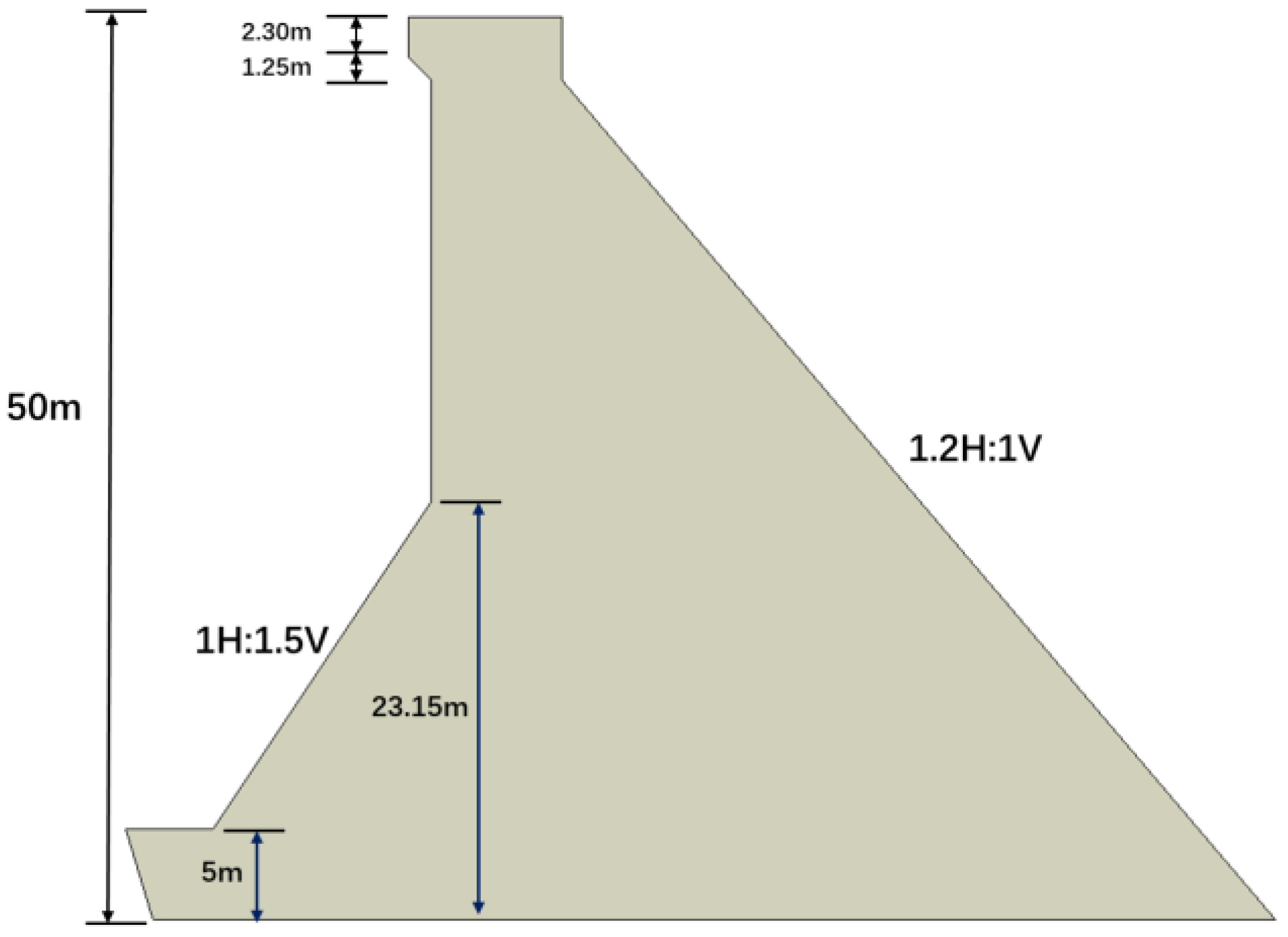
The case study presented in this paper is a project in the design phase. It is a concrete gravity dam with a curved axis, with a radius of 187 m. The profile was selected from the non-overflow section of the dam, and the geometric information was obtained from the design drawings. The maximum dam height is 50 m. The face of the dam body consists of a vertical and a 1H:1.5V slope, while the downstream face of the dam slope is 1.2H:1V. Specific geometric information is presented in
Figure 1. The normal operating water level is 1288 m at elevation. In the calculation and analysis of this paper, the downstream water depth was assumed to be 10 m.
2.2. The Finite Element Model of the Dam
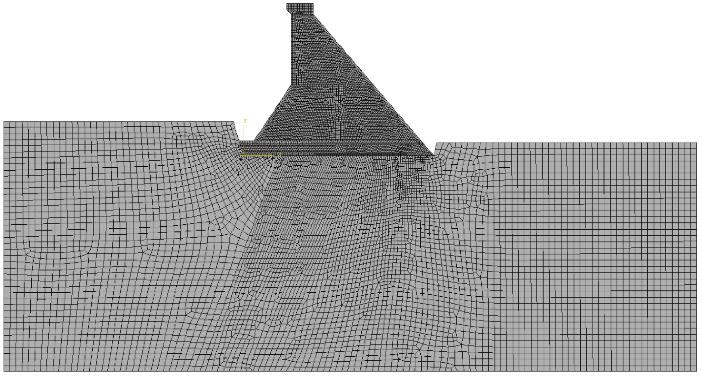
The finite element mesh of the basic profile used in the calculation is shown in
Figure 2. The maximum dam height is 50 m, and the length of the foundation in the model is 75 m, which extends 1.5 times the dam height from the dam heel to the upstream direction and extends 1.5 times the dam height from the dam toe to the downstream direction; the depth is 81 m, which extends the dam height. There are 12,721 nodes and 12,687 elements in the dam body and the foundation. For the dam, the average element size is 0.5 m. We adopt plane stress elements for the dam body and plane strain elements for the foundation. In this paper, the above two-dimensional dam profile model is selected for calculation. In this case, it is not possible to consider the three-dimensional dam interaction among monoliths and the valley effect.
2.3. Material Parameter Selection
For the values of elastic modulus, tensile strength, and compressive strength in CVC, we choose C25 concrete parameters under Chinese design codes [
22,
23,
24], referring to the research results of Tianying Liu et al. [
25], and convert them into corresponding parameters under US design documents [
26,
27], as shown in
Table 1. The specific conversion process is shown in
Appendix A.
The value of Poisson’s ratio of concrete is 0.2 in reference to Koyna Dam [
28].
According to the American Concrete Institute [
29], when no specific test value is available, the cohesion of concrete should be 0.1 times the compressive strength of concrete, and the friction coefficient should be 1.0.
As for the shear strength parameters between the concrete and bedrock, there is no clear experiment in the literature to show the difference and conversion relationship between the shear strength parameters between rock and concrete in the Chinese and American design documents [
30,
31,
32]. The shear parameters between the foundation and concrete are provided by Beifang Investigation, Design & Research CO. LTD in Tianjin, China.
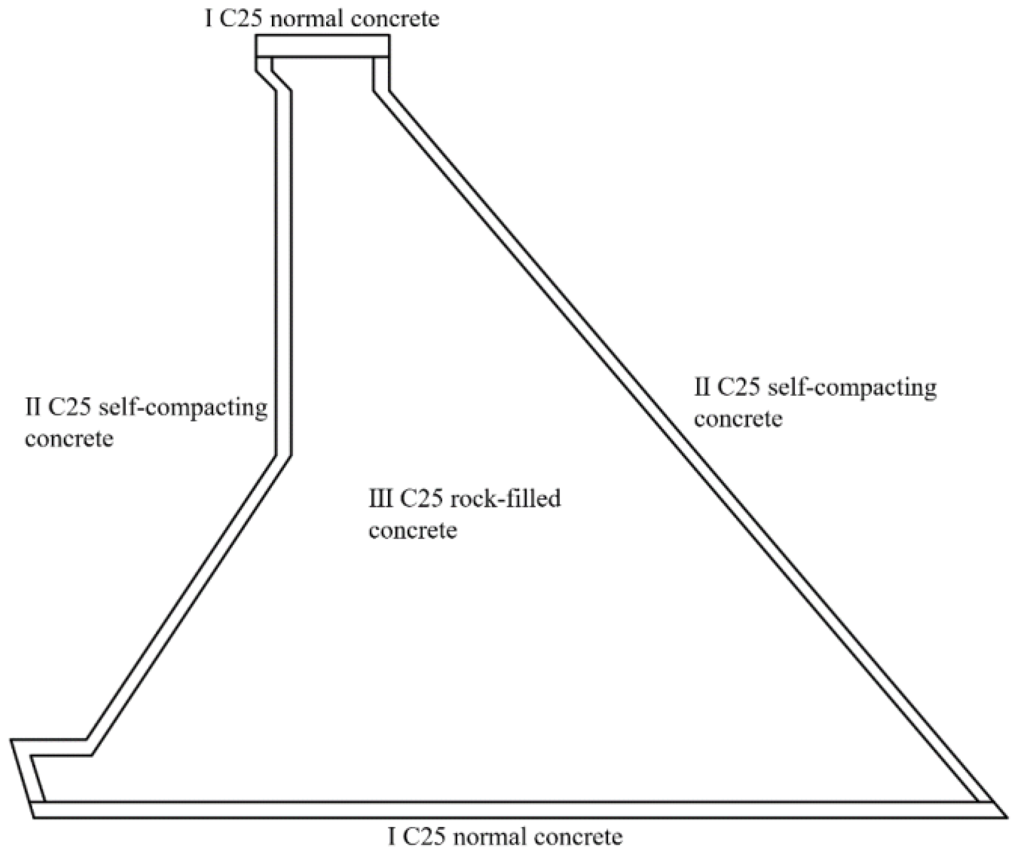
The material partition of the RFC dam scheme is shown in
Figure 3. Here, 1 m thick C25 self-compacting concrete is used as the impermeable layer on the upstream and downstream surfaces, 1 m thick C25 CVC is used as the transition surface on the base of the dam, 1.4 m thick C25 CVC is laid on the top of the dam, and C25 RFC is used for the main part of the dam.
The static material parameters of the dam body and the foundation are shown in
Table 2, and according to the US design documents [
30], the dynamic material parameters are shown in
Table 3. Among them, the shear strength of the dam refers to the parameters between the concrete body of the dam, and the shear strength of the bedrock refers to the parameters between the concrete and the foundation rock. All the foundation parameters are derived from geological survey data.
Based on the work of Liang et al. [
19], the elastic modulus of the RFC can be calculated using the following equations:
where
and
represent Poisson’s ratio and shear modulus of the reference matrix in spatially averaged composite Eshelby tensor;
f is the volume fraction of the inclusion;
represents the shear modulus of the surrounding composite;
and
are the homogenized results of the effective bulk and shear modulus of RFC at
;
and
represent the bulk and shear modulus, respectively;
and
are the shear and bulk modulus of the SCC at
;
and
are the shear and bulk modulus of the comparison solid at
;
is the homogenized result of the elastic modulus of RFC at
.
When the elastic modulus of rock and HSCC is 40 GPa and 21 GPa respectively, the elastic modulus of the RFC calculated using Equations (1)–(5) is 26.83 GPa. In this paper, conservatively, we set the elastic modulus of RFC to 1.2 times that of CVC, which is 25.2 GPa. In addition, according to the construction code of the RFC dam [
31], the unit weight of RFC is 2450 kN/m
3.
2.4. Seismic Input
Operational Basis Earthquake (OBE) and Maximum Credible Earthquake (MCE) are determined by seismic safety evaluation, with peak ground acceleration (PGA) values of 0.253 g and 0.701 g, respectively. The United States Geological Survey provides an earthquake risk map within the United States (USGS, 2014), and because the site is located in a region where earthquakes occur frequently, it is analogous to an area of California in the United States where earthquakes are more hazardous. According to the seismic risk map, the corresponding acceleration response spectra
,
for periods of 0.2 s and 1.0 s with a 50-year overshooting probability of 10% (return period of 475 years) and a 50-year overshooting probability of 2% (return period of 2475 years) can be obtained, as shown in
Table 4.
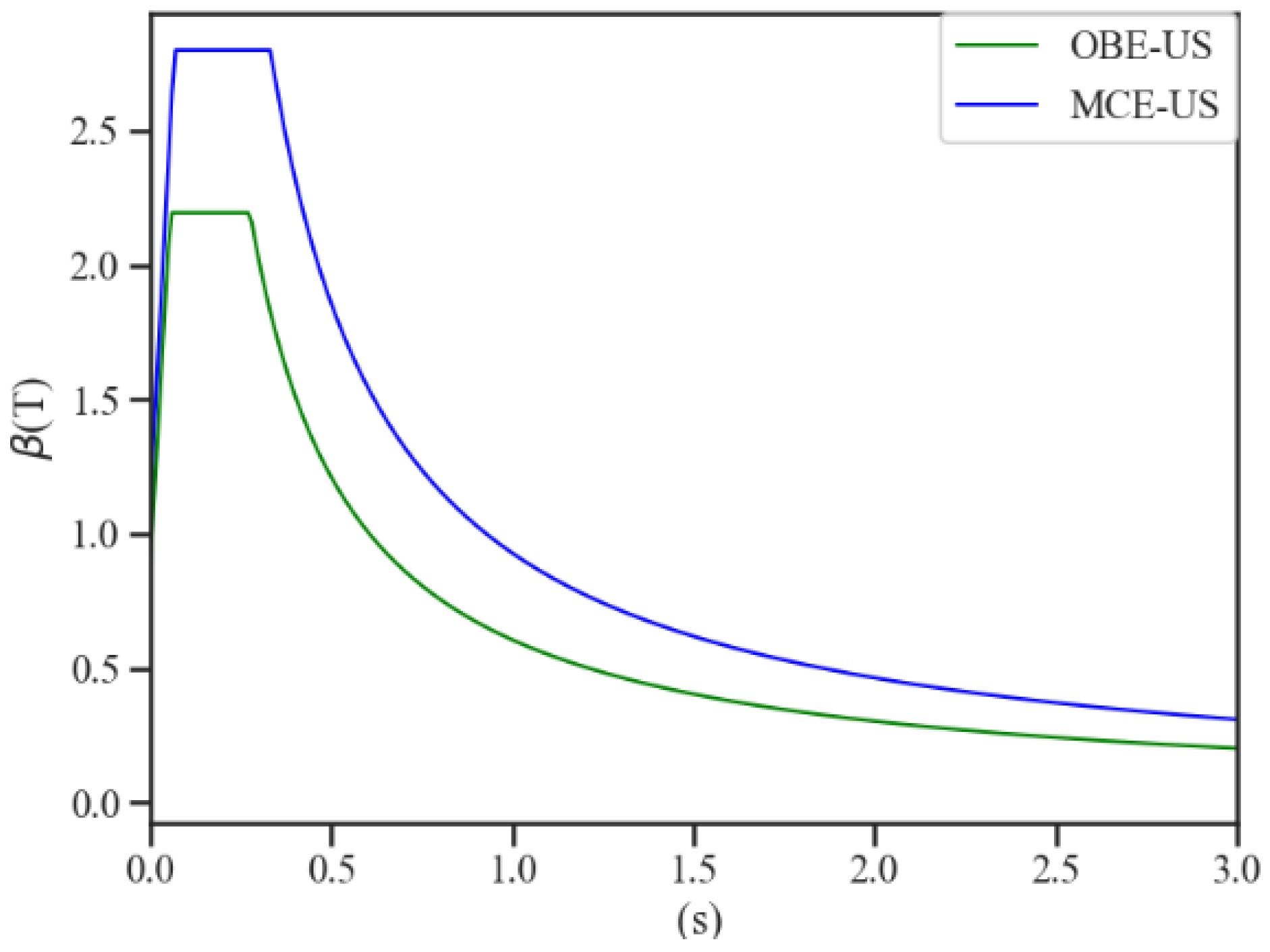
The US standard response spectrum formula for the horizontal direction of OBE and MCE levels [
30] is normalized (that is, the standard response spectrum formula is divided by PGA) and plotted in
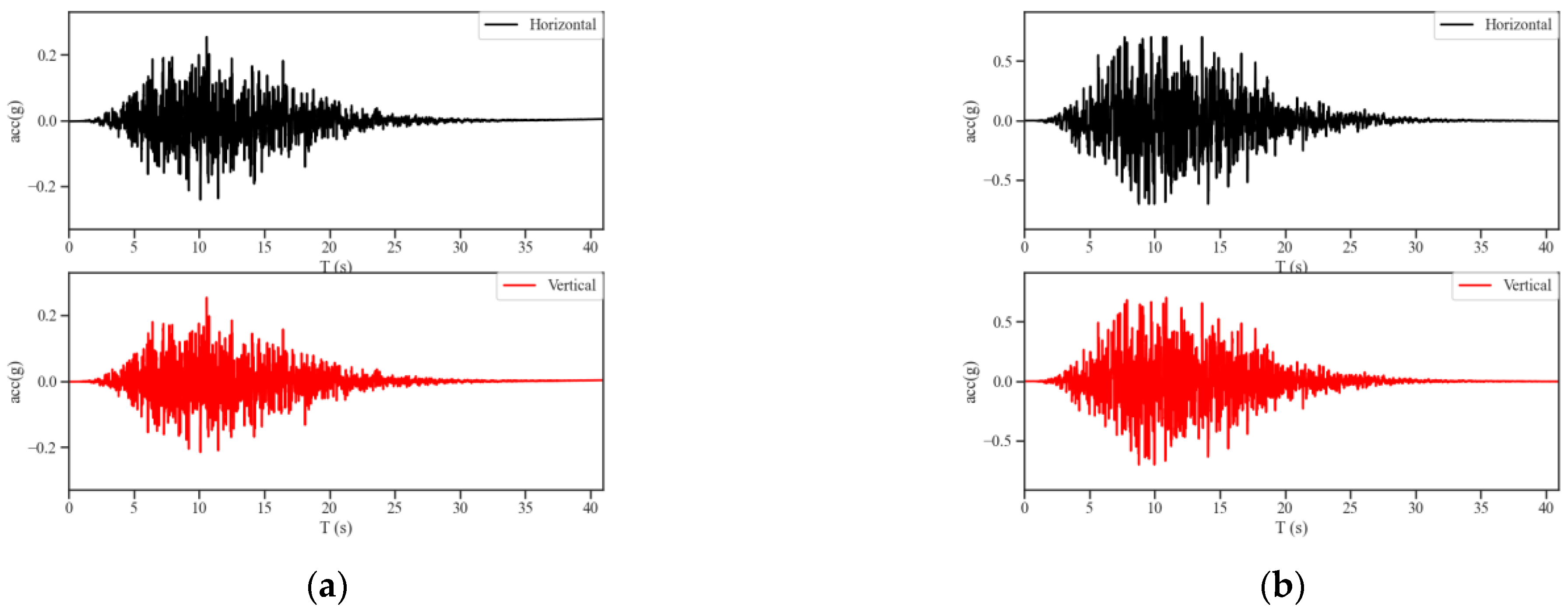
Figure 4. According to the standard response spectrum, the time history of ground motion used in the subsequent calculation is obtained, as shown in
Figure 5.
2.5. Other Loads
- (1)
Dead load of the dam.
- (2)
Upper and lower water pressure. The upstream water depth is 46 m, and the downstream water depth is 10 m.
- (3)
Lifting pressure. According to USACE EM1110-2-2200 [
32] (see pages 3–4 and 3–5 for details), the lifting pressure is calculated as follows:
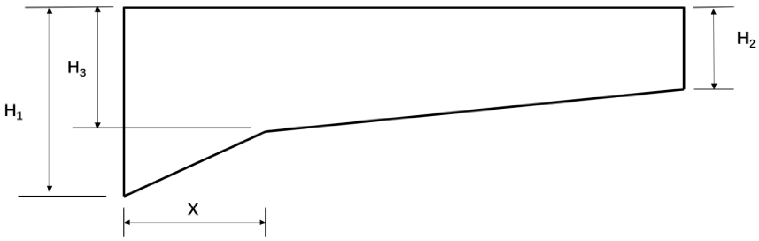
In
Figure 6, X is the distance from the drainage gallery to the dam heel, which is 13.43 m in this project; H
1 represents the upstream water level; H
2 represents the downstream water level; H
3 = H
2 + K(H
1 − H
2), and K is taken as 1/3.
- (4)
The hydrodynamic effects of the dam reservoir are modeled as an added mass of water moving with the dam using Westergaard’s formula:
where
p is the dynamic water pressure at a certain point on the dam surface,
is the mass density of reservoir water,
H is the depth of reservoir water in front of the dam,
Z is the height of the point above the dam foundation, and
is the acceleration of the joint point on the dam surface. It should be noted that the Westergaard added mass approach has limitations in the time-history analysis of dams because the added mass is constant but the actual hydrodynamic pressure changes in time as the dam structure responds to the seismic excitations. In addition, the Westergaard added mass approach ignores compressibility. However, for the comparative study in this paper, the method does not have a great impact on the results.
3. Methods
3.1. The Analysis Methods and Conditions of Strength Evaluation
In the design documents regarding seismic analysis of dams [
23,
30], there are usually three methods used to evaluate the strength of the gravity dam body, namely the static method, quasi-static method, and dynamic method. In the calculation, we generally adopt these methods to evaluate the seismic performance of the dam in turn.
The dynamic method is a method considering the seismic action according to the structural dynamic theory, which is widely used in the present mode superposition response spectrum method and time-history analysis. The mode superposition response spectrum method involves calculating the seismic response under each mode separately and then combining the seismic action under each mode together; that is, first the seismic response under a single-degree-of-freedom system is calculated, and then the results are combined to form the seismic response of the multi-degree-of-freedom structure. This method cannot reflect the change in the seismic response of the dam with time and cannot consider the different directions of force and displacement under different vibration modes when the vibration modes are combined and superimposed, so the calculation results are not accurate enough. The time-history analysis method can make up for these two shortcomings. The time-history analysis method involves taking the acceleration time history of the earthquake as the ground motion input, calculating the seismic response of the dam at each moment, and obtaining the response result of the dam every second through the form of step-by-step integration.
In this study, we use time-history dynamic analysis to study the seismic performance of CVC and RFC.
3.2. The Plastic Damage Model Used in the Nonlinear Analysis
For nonlinear analysis, the plastic damage model [
33] is used to represent the damage mechanism of the concrete. Combined with continuous damage mechanics and plastic theory, this model can simulate the plastic deformation of the stiffness degradation variable and the constitutive relation of concrete plastic damage which is not coupled and suitable for cyclic loading. The model uses two damage variables to describe the tensile and compressive failure under different damage states, respectively.
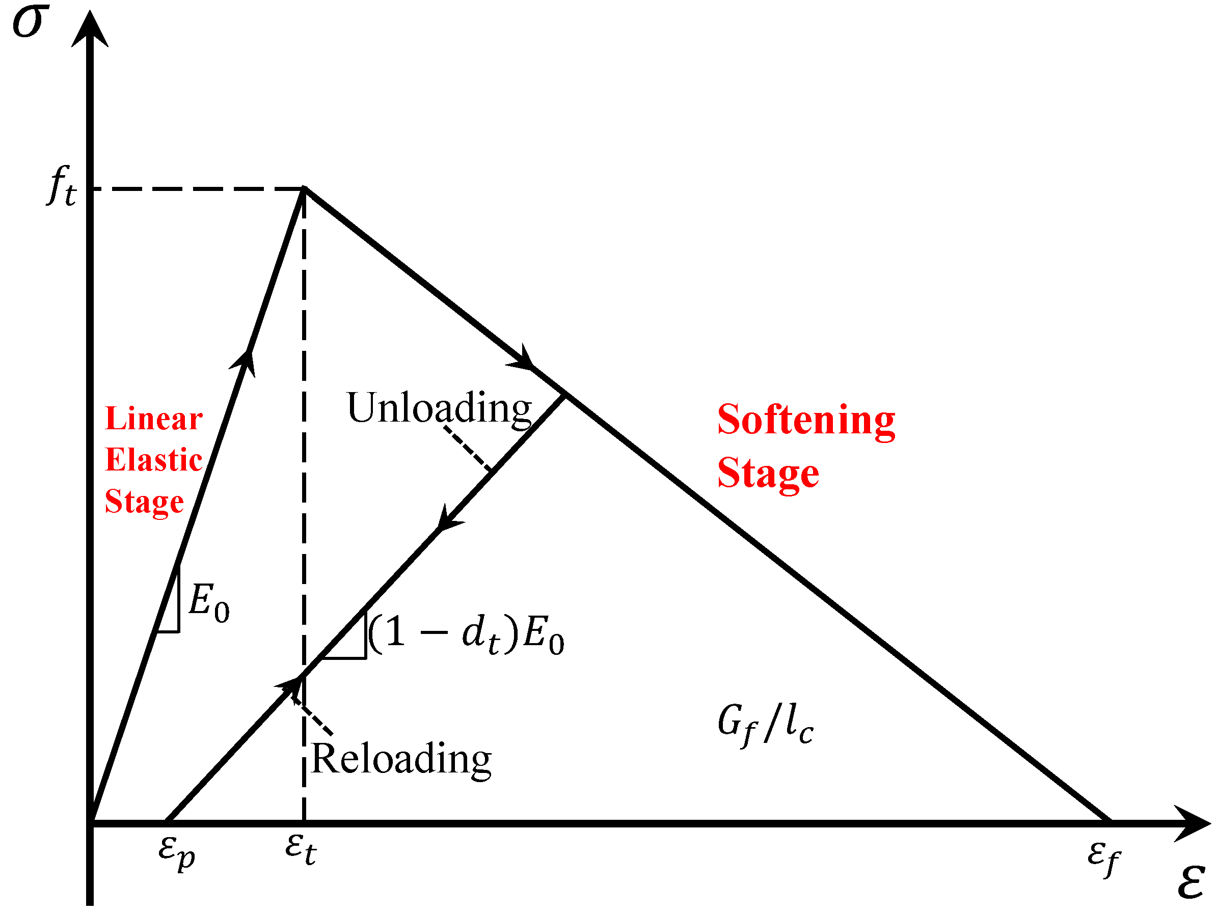
Given that the compressive strength of concrete is higher than its tensile strength, dam safety is usually controlled by seismic-induced tension stresses. Therefore, only the tensile damage of concrete is taken into consideration for simplicity [
34]. When the tensile stress of concrete does not reach the tensile strength, the concrete is in the linear elastic stage. After reaching the tensile strength, the stiffness of the concrete deteriorates and is in the softening stage. At a certain point in the softening stage, it is unloaded along the stiffness after degradation. After unloading to zero, there remains an unrecoverable strain including micro-cracks. During reloading, the load is applied along the uninstall path. Based on this theory, the constitutive relation of concrete is shown in
Figure 7, and it can be expressed as follows:
where
and
represent stress and strain, respectively;
is the initial elastic modulus; dt is the damage factor from 0 to 1 (fully damaged); G
f is the fracture energy;
represents the uniaxial tensile strength;
is the characteristic length of concrete; and
represent the maximum, limit, and equivalent plastic strains, respectively.
3.3. The Analysis Methods and Conditions of Anti-Sliding Ability
According to Section 6.2 of NB/T 35026-2014 [
22], the limit state of carrying capacity is generally adopted for checking calculations, in which the effects of dead weight, water pressure, lifting pressure, and silt pressure are multiplied by corresponding sub-coefficients.
where
is the structural importance coefficient,
is the design condition factor,
is the action effect function,
is the structure and component resistance function,
is the partial coefficient of permanent action,
is the partial coefficient of variable action,
is the partial coefficient of seismic action,
is the standard value of permanent action,
is the standard value of variable action,
is the representative value of seismic action,
is the standard value of geometric parameters,
is the standard value of material properties,
is the partial coefficient of material properties, and
is the structural coefficient.
Formula (8) is rewritten as Formula (9):
And let us write the left-hand side of this inequality as Equation (10).
For the anti-sliding stability review, we only need to calculate and then compare its size relationship with 1; if , it meets the requirements of the specification.
The rigid body limit equilibrium method is also adopted for anti-sliding stability analysis in the American design document. According to Sections 4–6 of EM 1110-2-2200 [
32], the method for calculating the safety factor of anti-sliding stability is shown in Equation (11).
where
N represents the resultant force perpendicular to the assumed sliding surface,
c is the cohesion strength,
L is the length of the dam foundation surface, and
is the internal friction angle.
4. Linear Elastic Simulation Results: Seismic Behavior of the Dam
This section presents the use of the time-history analysis method to calculate and analyze the seismic response of the dam section via ABAQUS, using the artificial acceleration time history generated by the inversion of the standard design response spectrum (
Figure 4) drawn according to the American design [
30] as input. A massless foundation model is used to simulate the dam–canyon interaction, and the design seismic time history is input uniformly on the boundary of the foundation. It should be noted that the massless foundation model does not take into account the absorption of seismic waves by the remote foundation, which may lead to greater structural effects in the system than in the actual situation. However, based on the comparative study in this paper, the use of this model is reasonable. The load includes the dam body weight, upstream and downstream hydrostatic pressure, dam foundation lifting pressure, and seismic excitation. The concrete material of the dam body and the rock mass of the dam foundation are considered linear elastic. In the calculation, the damping ratio of the calculation model is 5% under the OBE scenario and 10% under the MCE scenario.
4.1. Analysis of Natural Vibration Characteristics
In this section, the natural vibration characteristics of the dam are analyzed to provide the basis for dynamic analysis. The first 10 frequencies of the dam are shown in
Table 5, compared with the frequencies of the CVC dam. The frequencies of the RFC dam are close to those of the CVC dam in each vibrating mode, especially for the first two modes, which means the RFC dam has almost the same natural vibration characteristics as the CVC dam.
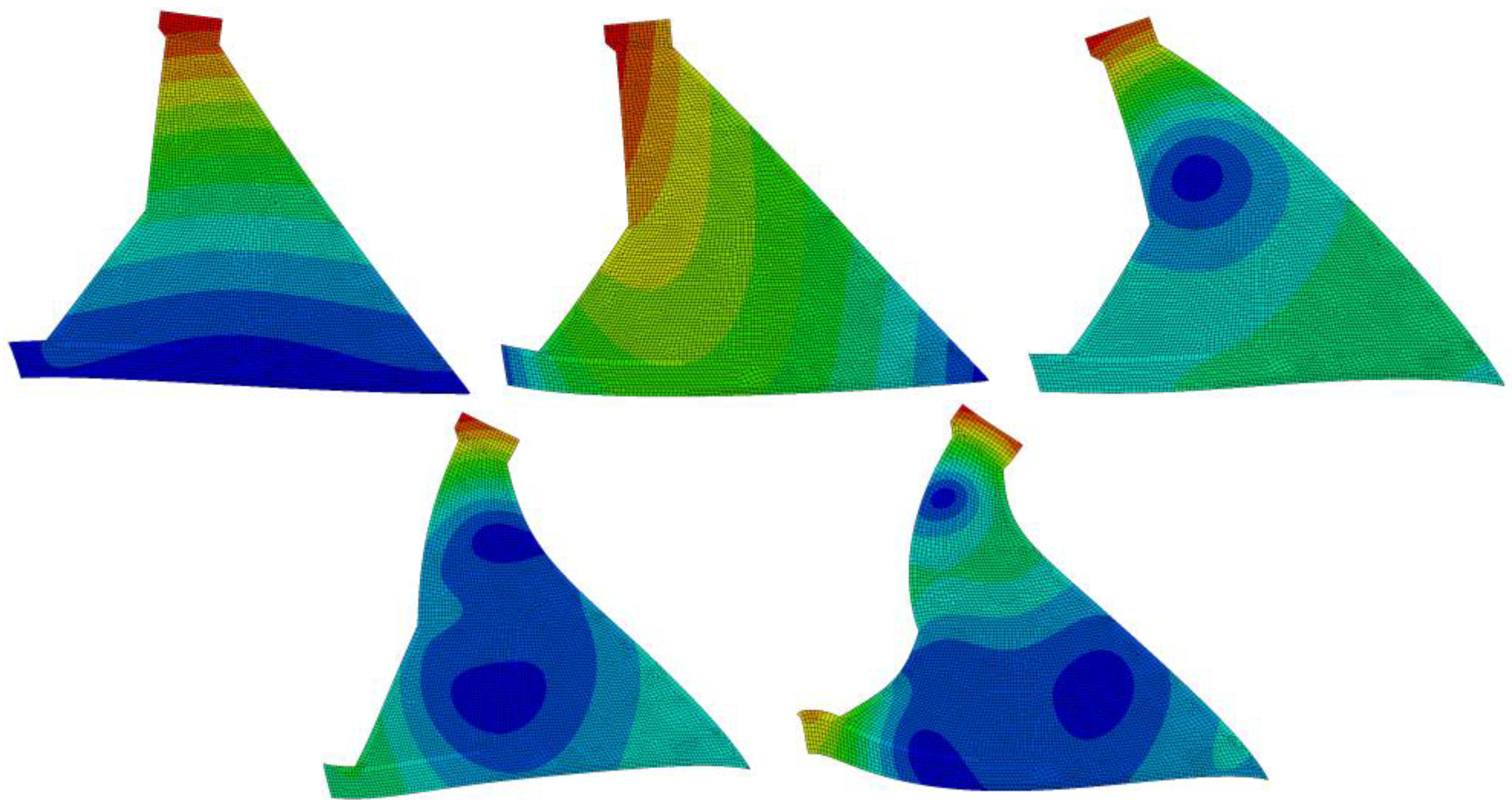
The first five vibration modes of the dam are shown in
Figure 8. The first vibration mode is mainly horizontal, and the second mode is simultaneously both horizontal and vertical, which conforms to the general dynamic characteristics of gravity dams.
4.2. Analysis of Linear Elastic Dynamic Response of Dam
- (1)
RFC dam
The maximum instantaneous displacement values of the dam body are listed in
Table 6, and the contour maps of the horizontal displacement are shown in
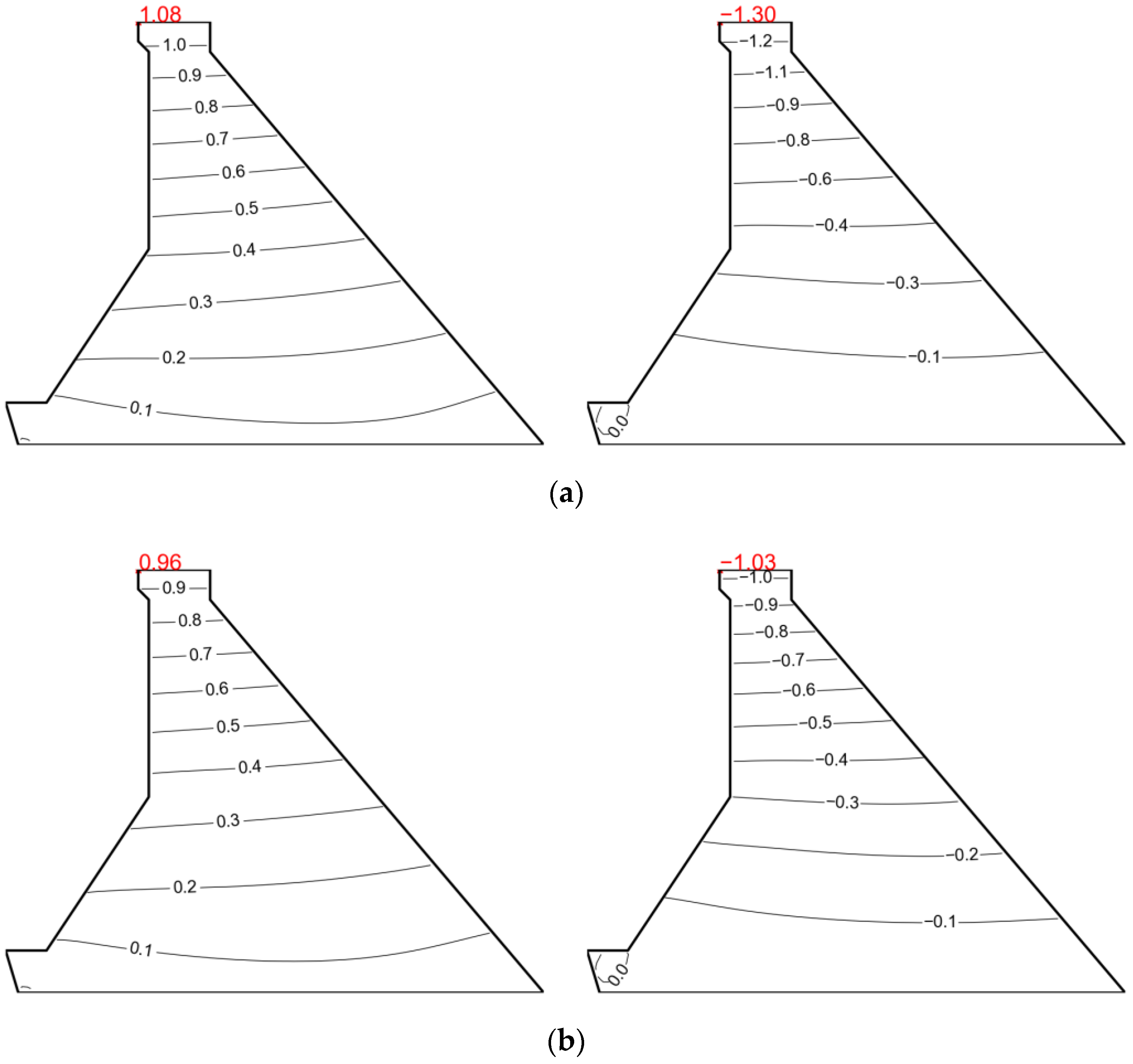
Figure 9. We can see that the distributions of horizontal displacement with different materials under the OBE scenario are the same. The same results can be obtained in extra cases for vertical components and with other input conditions (e.g., with MCE input).
- (2)
Dam stress
It can be seen from
Figure 10,
Figure 11,
Figure 12 and
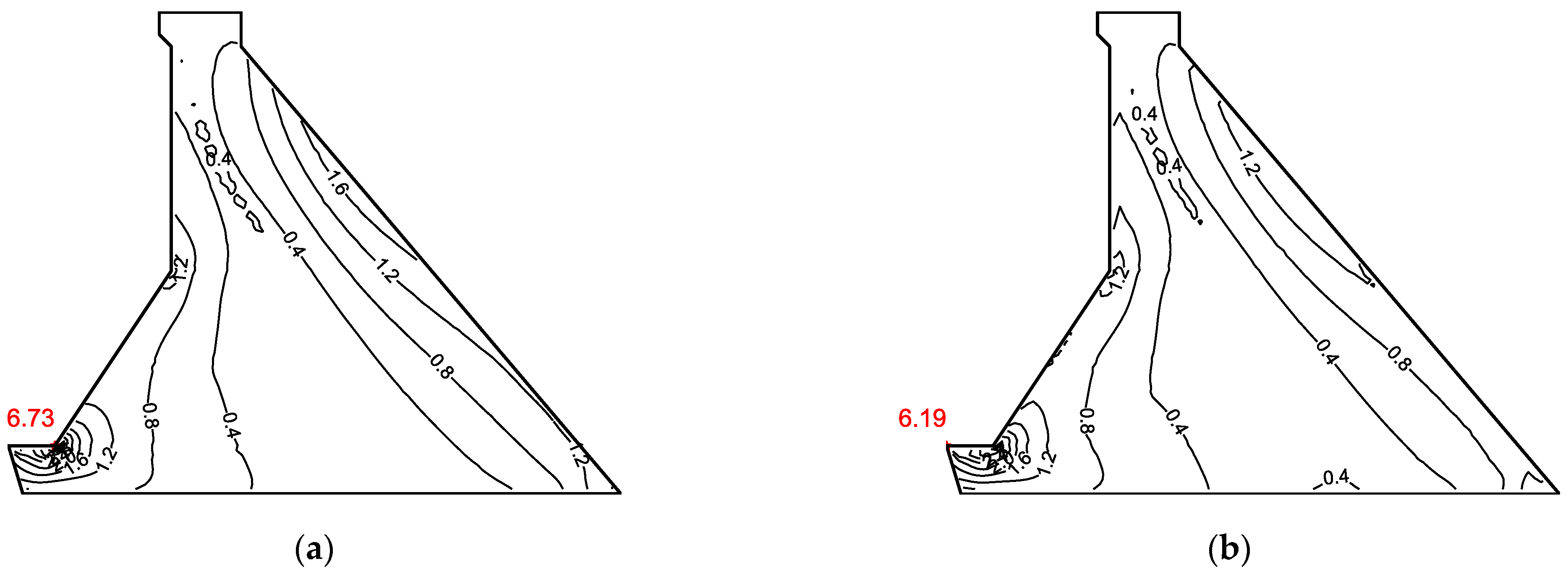
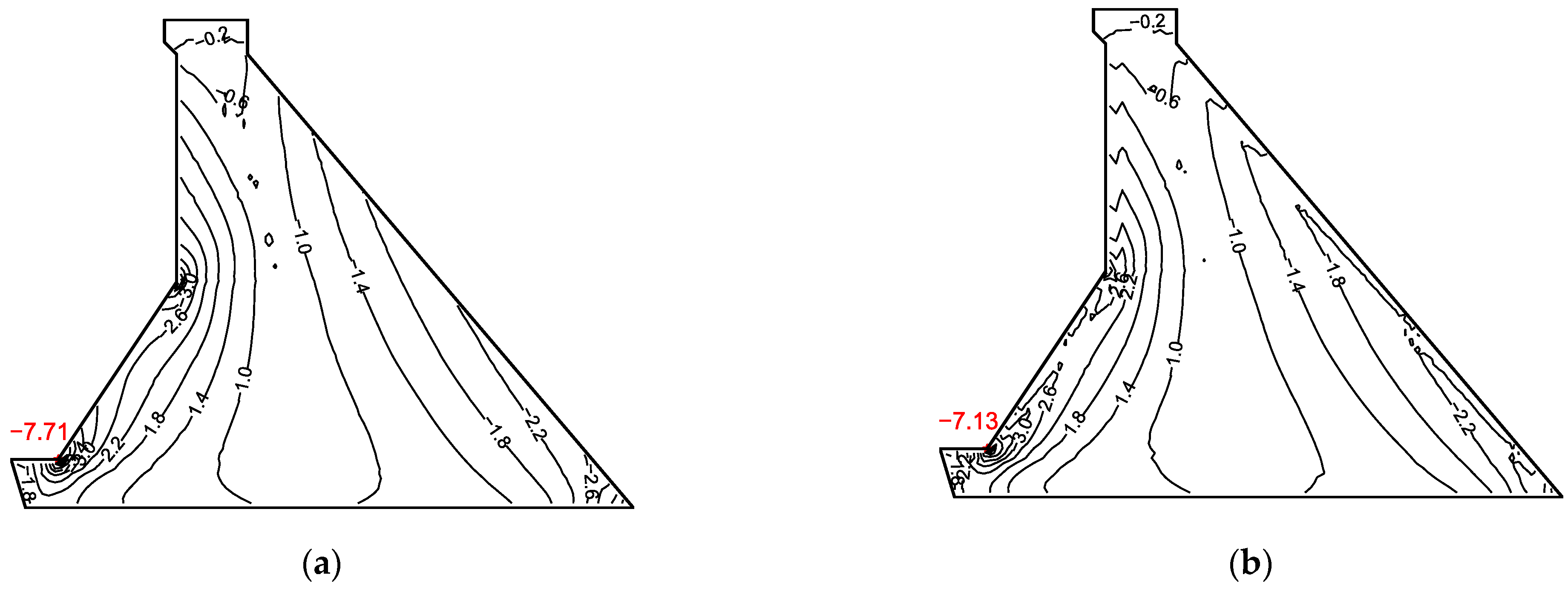
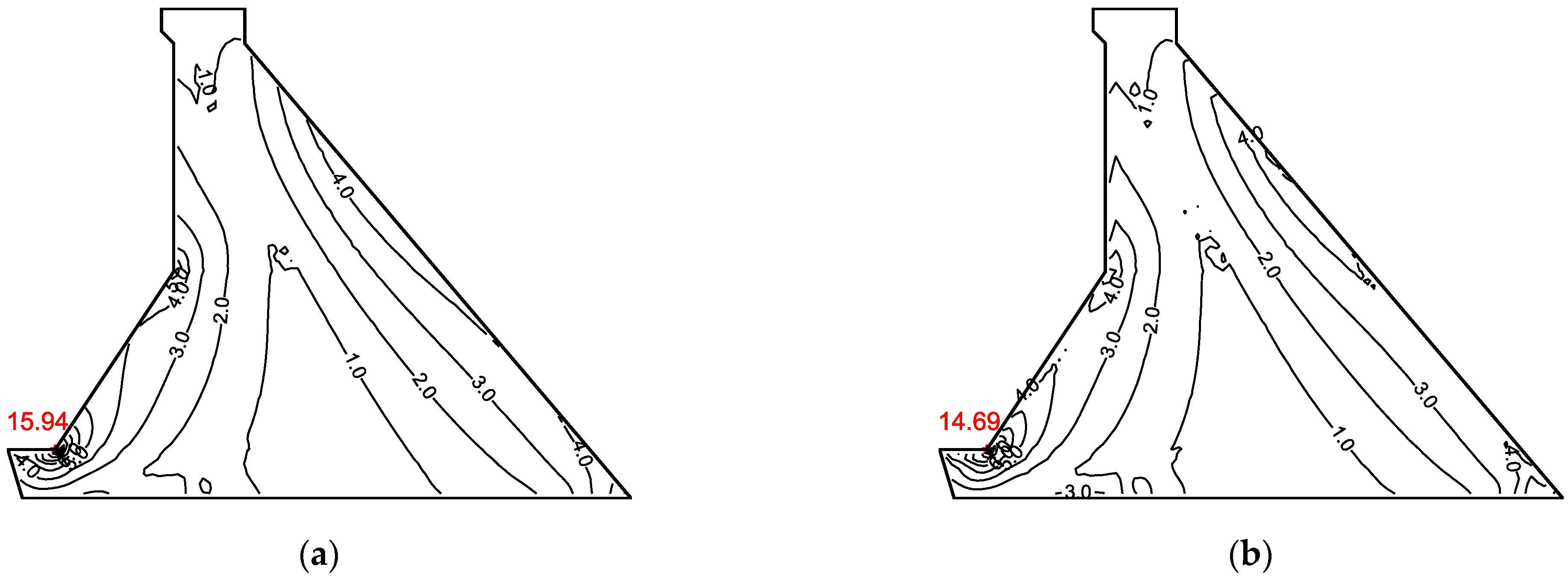
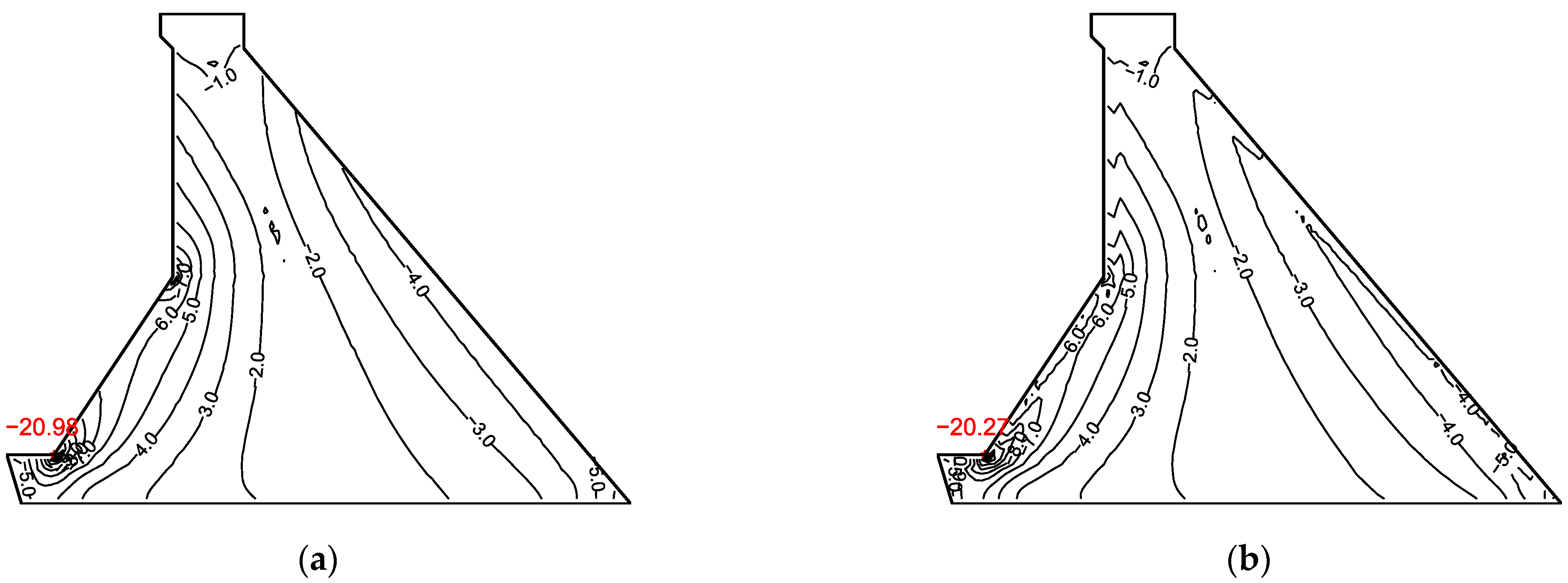
Figure 13 that the stress distribution in the dam body with two kinds of concrete materials is the same, and the high-stress area of the dam body is mainly concentrated in the upstream break slope, dam heel, and dam toe area. There is a large range of high-tensile-stress areas in the downstream slope of the dam body.
In terms of response, the extreme stress of the RFC dam is slightly lower than that of the CVC dam, and the overall stress level is also lower.
In the analysis mentioned above, we can see that Young’s modulus and density of RFC are both only slightly higher than those of CVC, which causes the fundamental natural frequency of RFC dams to be close to that of CVC dams. Therefore, the linear elastic analysis results of the RFC and the CVC dams are similar.
In addition, the dynamic response of gravity dams is particularly sensitive to the first and second natural frequencies. The fundamental frequencies of RFC and CVC dams are both ~0.2 s (
Table 5), with constant values of β (
Figure 4). Therefore, the input seismic waves of these two dam types have almost the same dominant components near the fundamental nature frequency. This explains why the linear elastic response of the RFC dam is almost the same as that of the CVC dam, with only a slightly smaller response.
4.3. Safety Evaluation of Linear Elastic Strength
The demand-to-capacity ratio (DCR), according to USACE EM 1110-2-6051 [
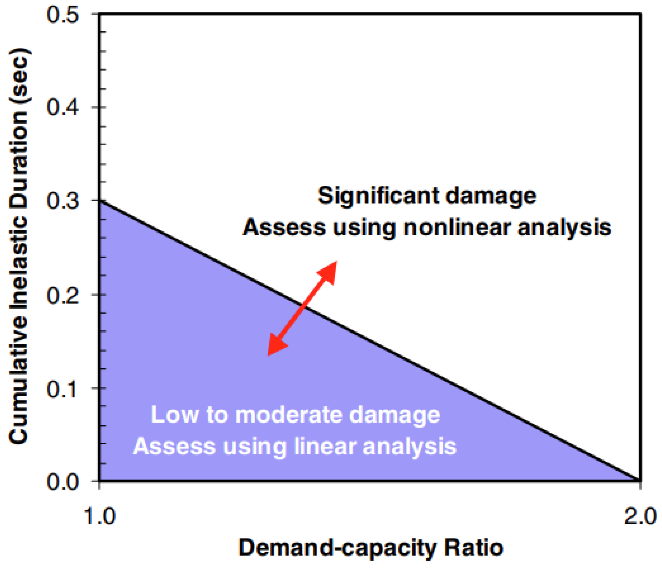
35] is used in this paper. The cumulative inelastic duration (CID) and performance curve are evaluation indicators.
The DCR is the ratio of requirements to capabilities. For the plain concrete used in this calculation, the DCR is the ratio of the principal stress required by the dam body to the static tensile strength of the concrete material. According to the DCR value, combined with the CID and performance curve, the dam dynamic response results can be divided into three performance levels:
- (1)
Minor or no damage. The dam response is considered to be within the linear elastic range of behavior with little or no possibility of damage if DCR ≤ 1.
- (2)
Acceptable level of damage. The dam will exhibit a nonlinear response in the form of cracking and joint opening if the estimated DCR > 1. The level of nonlinear response or cracking is considered acceptable with no possibility of failure if DCR < 2, overstressed regions are limited to 15 percent of the dam cross-section surface area, and the cumulative duration of stress excursions for all DCR values between 1 and 2 falls below the performance curve given in
Figure 14.
- (3)
Severe damage. The damage is considered severe when DCR > 2 or cumulative overstress duration for all DCR values in the range of 1 to 2 falls above the performance curves given in
Figure 14. In these situations, a nonlinear time-history analysis may be required, especially if the fundamental period of the dam falls in the ascending region of the response spectra.
Under OBE conditions, the dam stress level does not exceed the material strength of concrete in the main dam body (neglecting the stress concentration effect), which means the dam concrete material remains within the linear elastic range. Under MCE conditions, the principal tensile stress exceeds the strength of the concrete in some dam body areas, so it is necessary to evaluate DCR under MCE conditions to determine whether subsequent nonlinear analysis is necessary.
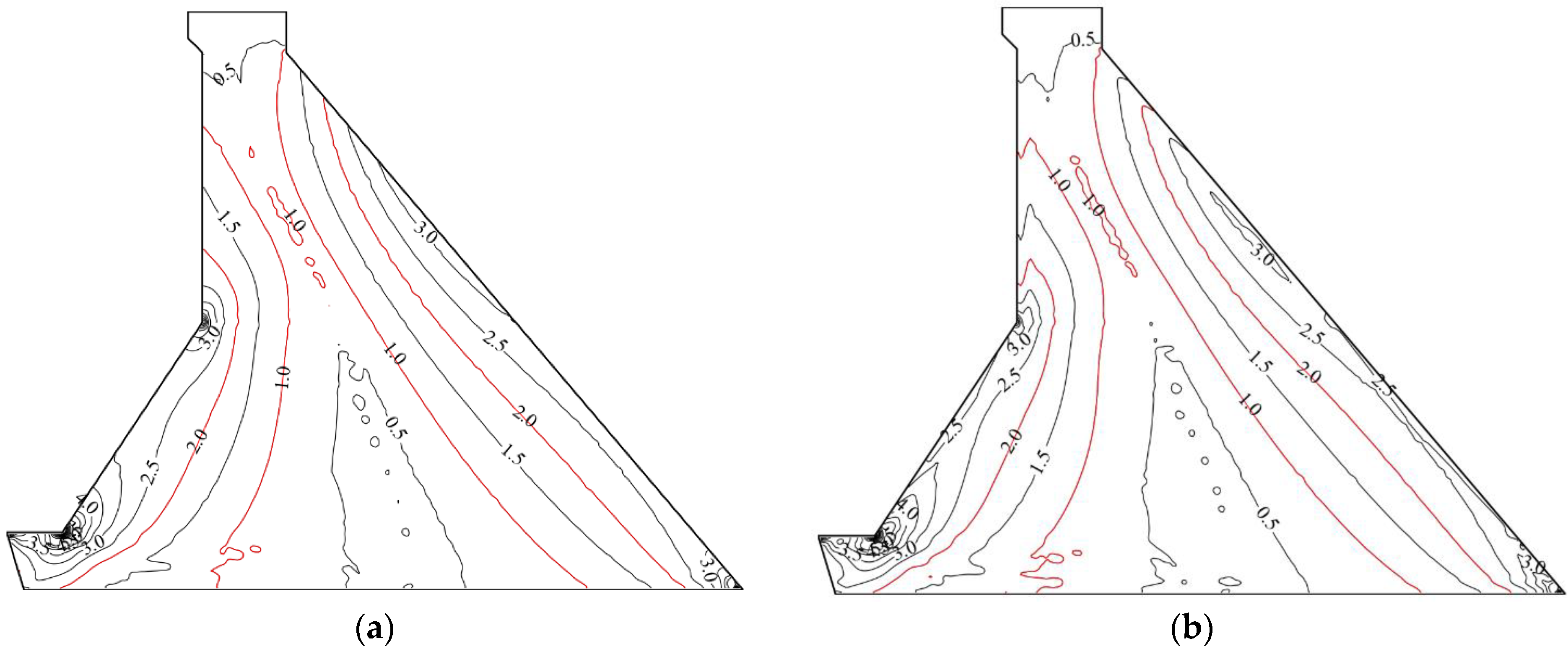
As can be seen from
Figure 15, there is an area of DCR > 2 in the dam body under MCE conditions, and the area of 1 < DCR < 2 in the profile is greater than 15% of the surface area of the dam section.
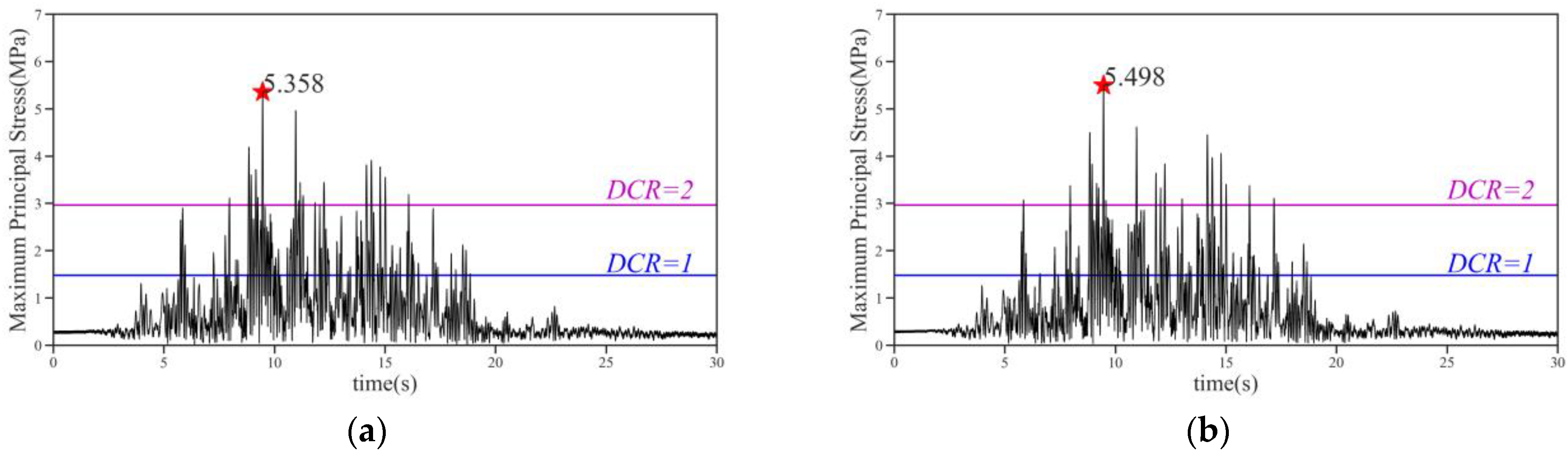
As can be seen from
Figure 16, the maximum principal stress of the dam body responds greatly between 7 s and 17 s, and the maximum principal stress of the dam body section substantially exceeds the dynamic tensile strength of concrete (2.22 MPa, see
Table 2) in many moments.
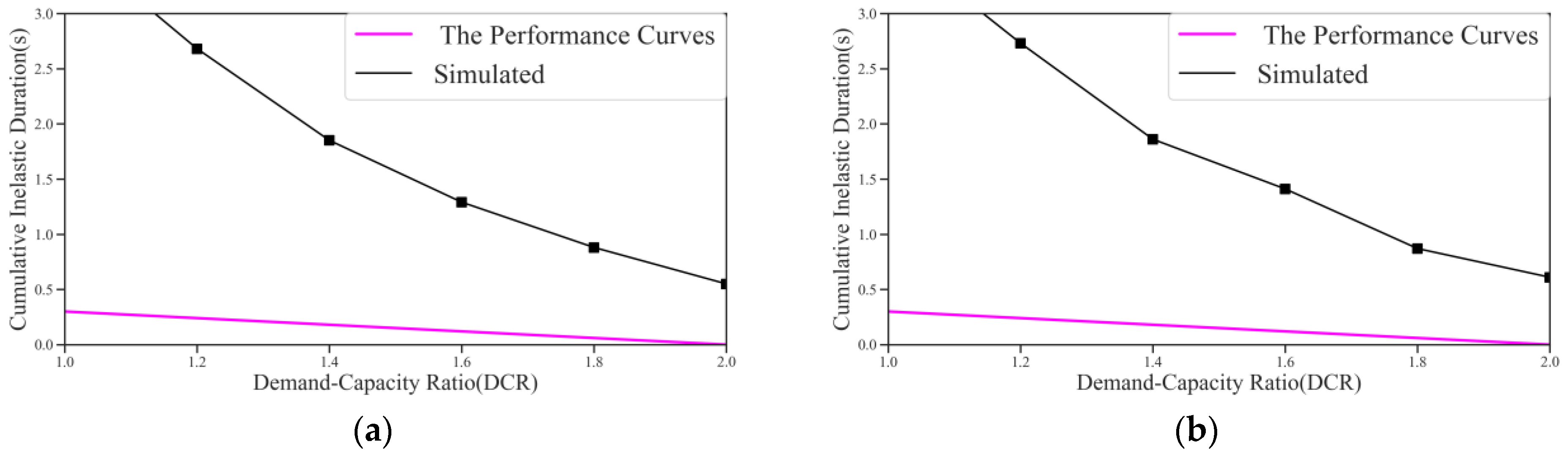
As can be seen from
Figure 17, the model performance curve of the dam is completely in the nonlinear region, and further calculation of the nonlinear performance of the dam body is necessary.
5. Nonlinear Analysis of the Dam
To simulate the nonlinear properties of dam concrete, ABAQUS commercial software was used. The concrete plastic damage model adopted in this software was the CDP model, which is based on isotropic assumption and combines damage mechanics and plastic theory.
5.1. Fracture Energy Selection of RFC
The technology of dam construction using RFC breaks through the compaction theory constraint of traditional continuous gradation and adopts “bulk rock-filled + high self-compacting performance concrete” to cement and realize RFC with 6–7 gradation or even larger particle size aggregate. Compared with CVC, the maximum aggregate size of RFC is larger. According to some existing tests and research results [
36], the aggregate size is positively correlated with the fracture energy of concrete. Beygi et al. [
37] and Giaccio and Zerbino [
38] found that the strength, size, shape, and surface texture of aggregate have significant effects on fracture energy and cracking degree. Hillerborg [
39] analyzed the influence of the maximum particle size of aggregate on the fracture energy and found that with the increase in the aggregate particle size, the fracture energy tended to increase. Mihashi et al. [
40], Bažant and Oh [
41], Zhao et al. [
42], and Trunk et al. [
43] also summarized the same trend. To simulate the relationship between the fracture energy and the maximum particle size of the aggregate, they introduced a power function. Issa et al. [
44] observed that the fracture energy increased monotonically with an increase in the maximum particle size of the aggregate. Zhou et al. [
45] systematically tested the influence of different maximum particle sizes of aggregates on the fracture performance of high-strength concrete and found that the fracture energy increased with an increase in the maximum particle size of aggregates. According to the above research results, it can be inferred that the fracture energy of RFC is greater than that of CVC.
As for the fracture energy of RFC, according to the experimental results of Li [
46], the post-processing correction of the test data shows that for an RFC specimen of 0.45 × 0.45 × 1.9 m, the type I fracture energy is 288.2 N/m, and the measured type II fracture energy of RFC is generally about ten times the type I fracture energy. Type I and type II fracture energies have different behaviors in different parts of the dam, so the two kinds of fracture energy may be different when nonlinear failure occurs in the dam. In summary, the fracture energy of the dam should be greater than the type I fracture energy. In addition, the size effect of dam concrete should also be taken into account. Although no scholars have given the relationship between the fracture energy and the size of RFC specimens, we can make a reasonable prediction. According to the test results of Zhang [
47], when the thickness of specimens is the same, the fracture energy will increase to 1.2~1.3 times when the length and height of specimens are slightly increased. For the relationship between the test results of Li [
46] and the fracture energy of the real RFC dam, this section takes the fracture energy of the real RFC dam as 1.4 times the test result.
In summary, it can be inferred that the fracture energy of an RFC dam is greater than 400 N/m. As for CVC, the fracture energy provided by Beifang Investigation, Design & Research CO.LTD is 262 N/m. For safety reasons, the fracture energy of RFC is set as 400 N/m, which is conservative. So, the fracture energy of RFC is about 1.5 times that of CVC.
5.2. Nonlinear Damage Result
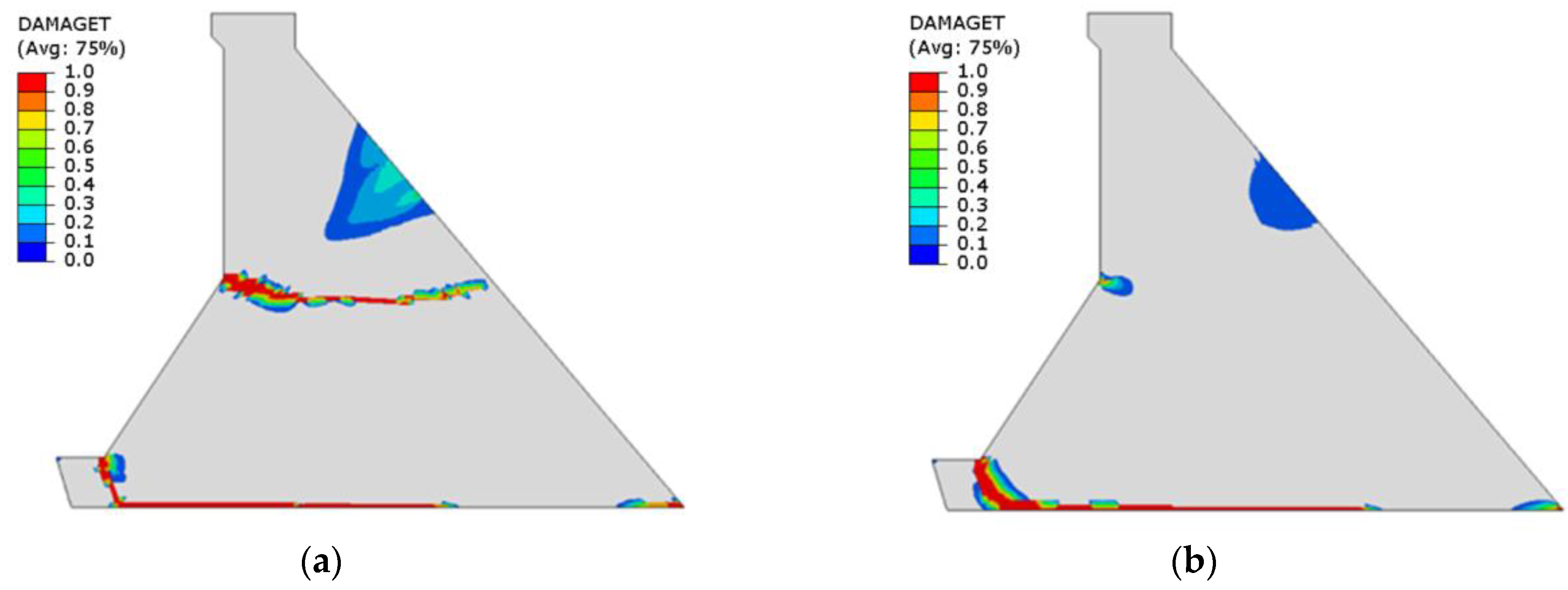
As can be seen from
Figure 18 under the massless foundation model, the application of RFC can greatly reduce the damage degree and damage area. When the CVC material is used, the dam body has penetrating damage between the upstream break slope and the downstream dam face, and there is a large area of damage in the middle height area of the dam. However, when RFC is used, the damage area at the upstream break slope is only 1/10 of the dam thickness, and the damage degree is reduced.
There are large-diameter stones in RFC dams. According to previous research [
39], fracture energy is positively correlated with stone size. Therefore, the fracture energy of RFC dams is greater than that of CVC dams. From a physical mechanism perspective, since RFC is a three-phase medium, that is, HSCC, rock, and ITZ, the rock is wrapped, dispersed, and suspended in the HSCC, and the ITZ is a weak layer between the rock and the HSCC. So, seismic waves always reach the large rocks in RFC dams, and the crack always propagates via the boundaries of rocks (ITZ) instead of through the rocks, which shows a relatively higher resistance to earthquakes.
6. Safety Evaluation of Anti-Sliding Stability
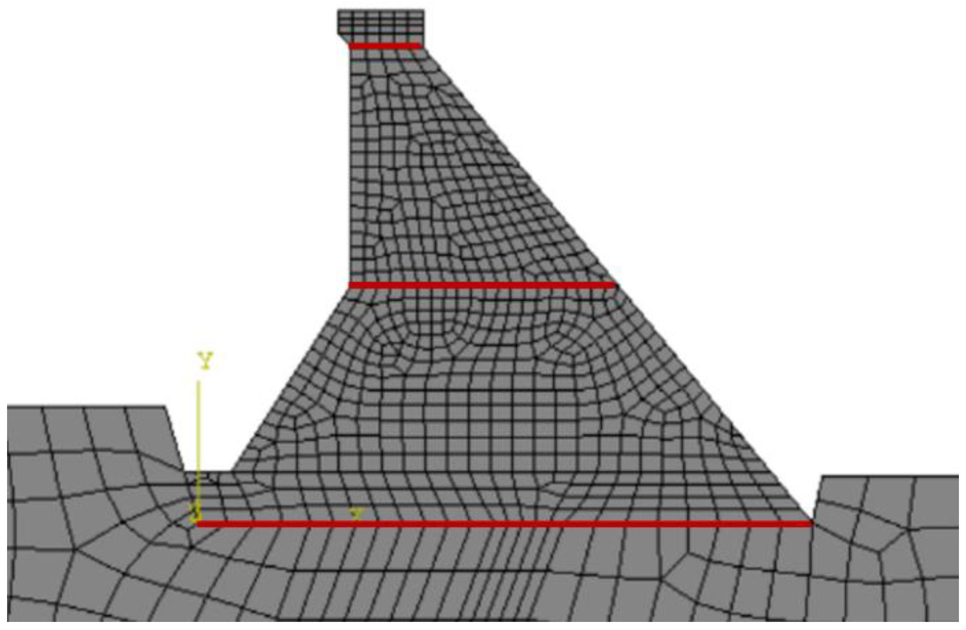
Three anti-sliding stability calculation layers are selected, namely the foundation surface, upstream broken slope plane, and downstream broken slope plane. The specific positions are shown in
Figure 19.
The safety factor method is used. The minimum sliding coefficient under OBE conditions is 1.7, and the minimum sliding coefficient under MCE conditions is 1.3.
In the process of time-history analysis, we calculate the safety factor of all levels at each seismic moment and check whether it is greater than the allowed value. If the calculation result of the safety factor is greater than 10, it is treated as 10, and the result is drawn into a time-history curve, that is, the time-history diagram of the safety factor of anti-sliding stability.
The instantaneous minimum values of safety factors of anti-sliding stability at all levels of the profile under OBE and MCE conditions are shown in
Table 7, along with time-history diagrams of safety factors at all levels of the dam body profile.
Under OBE conditions, the three typical layers of the CVC dam and RFC dam can pass the anti-sliding stability check, and there is little difference in safety coefficient between them. The safety margin of the RFC dam against sliding is higher on the downstream broken slope. On the foundation surface, the safety margin of the CVC dam against sliding is higher.
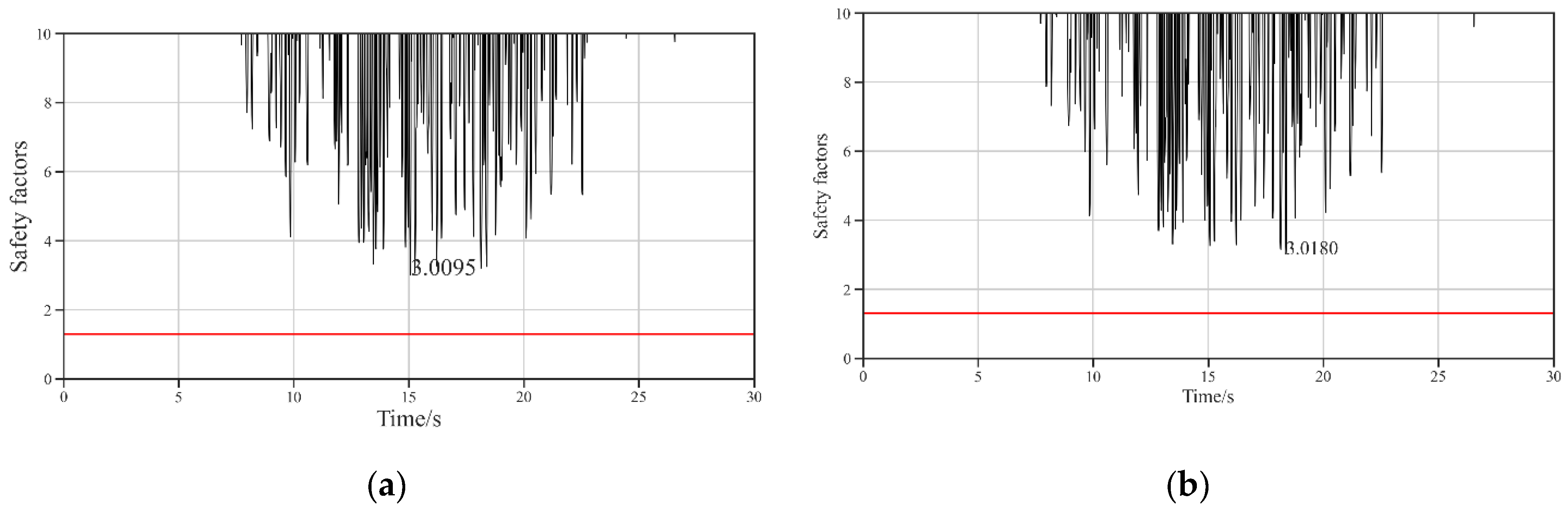
As we can see, under MCE conditions, the three typical layers of the CVC dam and RFC dam can pass the anti-sliding stability check, and the safety coefficient does not differ between the two. The safety margin of the RFC dam against sliding is higher on the downstream broken slope. There is almost no difference in the anti-sliding safety margin between the RFC dam and the CVC dam on the foundation surface and upstream broken slope. The time-history diagrams of safety factors at all levels of the dam body profile are shown in
Figure 20.
In summary, in terms of anti-sliding stability, there is no situation in which the safety factor of three typical layers is less than the allowable value.
The difference in anti-sliding stability between the RFC dam and the CVC dam is not particularly large. Considering that the shear strength of RFC is better than that of CVC, and the shear strength of the two is taken as the same in numerical simulation, this conclusion is conservative.
7. Discussion
Under the same loadings, the results show that the RFC dam exhibits similar responses in terms of natural vibration characteristics and seismic analysis. As shown in
Figure 15, the overstress area is mainly concentrated in the vicinity of the break of the upstream and downstream slopes, which is consistent with the results of Corai and Maity [
48]. As for the damage analysis, there are damaged areas in the downstream slope at the middle elevation, the break of the upstream slope, and the base of the RFC dam. Some research has been conducted on the nonlinear seismic analysis of CVC dams, and the results also show such a phenomenon [
49,
50]. According to the phenomenon of less damage in the RFC dam model, the main reason is that RFC has greater fracture energy, and more energy is required to damage RFC. However, the reason for the larger fracture energy of RFC is that from the perspective of the physical mechanism, since RFC is a three-phase medium, when the damage begins to develop in RFC, the cracking will develop along the weaker ITZ around the rocks. In this process, the energy of cracking is lost, so the cracking development is slower.
To facilitate the comparison, a two-dimensional gravity dam model and a simplified consideration of the Westergaard model were used in the simulation. Consistent with the hypothesis about hydrodynamic pressure and the assumption of 2D geometry in this paper, Nguyen [
51] proposed a procedure with the combination of Westergaard added mass to analyze a two-dimensional gravity dam considering soil–structure interaction. Due to its simplicity and conservative estimation, the Westergaard model is still widely used in the current seismic analysis of concrete dams. More and more researchers have studied the realistic seismic performance of concrete dams based on three-dimensional models and acoustic–solid coupling reflecting the interaction between the dam and the reservoir. Nikkhakian et al. [
52] carried out two- and three-dimensional nonlinear analyses to investigate the effects of canyon shape. The results show that two- and three-dimensional dam–reservoir–foundation coupled systems may lead to partly different results. Wang et al. [
53] also carried out a seismic response analysis of a gravity dam based on a three-dimensional model with the acoustic–solid coupling method compared with a two-dimensional model and found that there are some differences in damage level between the two models. Admittedly, these assumptions affect the response of the structure. Nevertheless, maintaining the same assumption, we can also compare the differences in seismic response between the RFC dams and CVC dams and obtain some conclusions worth exploring. Based on this paper, we can deeply discuss the seismic performance of RFC dams under the dam–foundation–reservoir system to depict the differences between RFC dams and CVC dams in detail.
8. Conclusions
Since the RFC technology was invented in 2003, it has developed rapidly in China and gradually gained international recognition. In this study, the time-history analysis method and massless foundation model were used to carry out dynamic calculations on a 2D finite element model of a gravity dam body with RFC and CVC to evaluate the safety of the dam body strength and anti-sliding stability. The following conclusions were reached:
- (1)
In terms of linear stress response, due to the increase in elastic modulus, the model stiffness of the RFC dam is larger, and its deformation and stress are smaller under the same load. Under the OBE and MCE scenarios, the stress distributions of the CVC dam and RFC dam are roughly the same, but the extreme stress value and stress level of the RFC dam are smaller than those of the CVC dam.
- (2)
Both models can pass the anti-sliding stability check. Under the OBE scenario, the safety margin of the CVC dam on the foundation surface is larger. Under the MCE scenario, the safety margin of the RFC dam on the foundation surface is larger.
- (3)
In terms of nonlinear calculation, compared with CVC dam, the damage degree and damage area of RFC dam are greatly reduced, since the larger fracture energy of RFC means that the energy required for damage is larger, so the damage area is smaller under the same input.
In summary, according to the geometry calculated, all the assumptions and material properties, and the seismic records used in this model, the performance of the RFC dam is better than that of the CVC dam, and the damage caused by earthquakes is less.
The value of RFC material is conservative, and the properties other than the two factors of elastic modulus and fracture energy improved by the addition of RFC are not considered. Therefore, compared with the numerical simulation results, the RFC material has a better performance in seismic performance in actual engineering. In the calculations of this study, it can be inferred that the current seismic codes for CVC dams are suitable for RFC dams.
The above discussions are only based on a case study for the dam using a simplified numerical simulation with specific material properties, according to previous studies and conservative estimation, and a specific seismic load record. It should be pointed out that the model parameters in this paper are based on basic scenarios. If more complex conditions are considered, such as load and boundary conditions and material parameters, the results would be more complex.
Based on the most advanced experimental data and some theoretical derivation formulas of current research on RFC, this paper gives some guidelines for selecting material parameters of RFC. However, at present, some more in-depth research on the material properties of RFC is underway or still in the preliminary stage. Therefore, it may be necessary to study the seismic performance of RFC in a more comprehensive and in-depth way based on experiments and numerical simulation in the future. Specifically, for further research, specific lab experiments and microscopic simulations need to be conducted, combined with more engineering applications to verify the reliability of these possible mechanisms and have a better understanding of the seismic performance of RFC dams.
Author Contributions
Conceptualization, Y.X. and F.J.; funding acquisition, Y.X. and F.J.; investigation, Y.X. and F.J.; software, C.T. and X.H.; supervision, Y.X. and F.J.; visualization, C.T. and X.H.; writing—original draft, C.T. and Y.X.; writing—review and editing, X.H., Y.X. and F.J. All authors have read and agreed to the published version of the manuscript.
Funding
This research was funded by the National Natural Science Foundation of China (Grant No. 52192672, 52192675, 52039005, 52339007) and State Key Laboratory of Hydroscience and Engineering (Grant No. 2021-KY-04, 2022-KY-01).
Data Availability Statement
Data and models used in this paper may be available to interested researchers upon request.
Acknowledgments
We thank Haiyan Yang and Desheng Yao from Beifang Investigation, Design & Research CO. LTD for their help and discussion.
Conflicts of Interest
The authors declare no conflicts of interest.
Appendix A. Chinese and American Concrete Parameter Conversion
The Chinese code for the Design of Concrete Structures (GB 50010-2010) [
24] is used to convert the values of relevant mechanical properties parameters of concrete in this section. The United States specifications are “Standard Practice for Making and Curing Concrete Specimens in the Field” (ASTM C31) [
26] and “Standard Test Method for Compressive Strength of Cylindrical Concrete Specimens” (ASTM C39) [
27]. The difference between the codes in the two countries mainly lies in the size of the specimen and the requirements for the guaranteed rate. The Chinese code stipulates that a cube specimen with a side length of 150 mm is used for the test, while the US design documents usually use a φ150 × 300 mm cylinder specimen for the test.
According to the Chinese code, the standard compressive strength value of the cube
is the compressive strength value with a 95% guarantee rate measured using the standard test method at 28d age under standard conditions, and the specific calculation method is shown in Equation (A1):
where
is the standard value of the compressive strength of the cube,
is the average compressive strength (MPa) of the specimen obtained from the test of concrete with a specified strength grade, and
is the standard deviation (MPa) of the compressive strength of the specimen. The values of the standard deviation of concrete under different strength grades in Chinese standards are shown in
Table A1.
Table A1.
The standard deviation of concrete of different strengths under Chinese specifications.
Table A1.
The standard deviation of concrete of different strengths under Chinese specifications.
| Strength Grade | C15 | C20 | C25 | C30 | C35 | C40 |
|---|
| Standard deviation (MPa) | 4.8 | 5.1 | 5.4 | 5.5 | 5.8 | 6.0 |
According to the research results of Shi Zhihua et al. [
54], the relationship between the compressive strength of the American standard concrete cylinder
and the standard compressive strength of the cube is approximately given as
. The American standard also uses standard deviation to control the guarantee rate of concrete strength, but its guarantee rate is not uniform and is related to the quality of concrete. The standard deviation of concrete strength of different control standards is shown in
Table A2. According to the US design document [
26,
27], when the specified concrete compressive strength
is less than or equal to 35 MPa, the required average compressive strength
is the greater value of the result calculated according to Equations (A2) and (A3):
Table A2.
The standard deviation of concrete strength under US design documents.
Table A2.
The standard deviation of concrete strength under US design documents.
| Excellent | Very Good | Good | Ordinary | Bad |
|---|
| Less than 2.8 MPa | 2.8~3.4 MPa | 3.4~4.1 MPa | 4.1~4.8 MPa | Greater than 4.8 MPa |
In the conversion of concrete compressive strength parameters under the two national norms, let under the US design documents be equal to under the Chinese design codes, and then calculate the corresponding concrete compressive strength of the cube specimen according to Formulas (A2) and (A3), and then multiply the result by 0.8 to obtain the compressive strength of the cylinder specimen under the US design documents.
The tensile strength
and elastic modulus
can be expressed as follows [
26,
27]:
References
- Jin, F.; An, X.H. Construction Method for Rock-Filled Concrete Dam. China Patent CN ZL03102674.5, 25 January 2006. [Google Scholar]
- Jin, F.; Huang, D.; Lino, M.; Zhou, H. A Review of Rock-Filled Concrete Dams and Prospects for Next-Generation Concrete Dam Construction Technology. Engineering 2023, in press. [Google Scholar] [CrossRef]
- Xu, X.; Liang, T.; Yu, S.; Jin, F.; Xiao, A. Mesoscopic thermal field reconstruction and parametrical studies of heterogeneous rock-filled concrete at early age. Case Stud. Therm. Eng. 2024, 53, 103800. [Google Scholar] [CrossRef]
- Shah, S.P.; Lomboy, G.R. Future research needs in self-consolidating concrete. J. Sustain. Cem.-Based Mater. 2015, 4, 154–163. [Google Scholar] [CrossRef]
- Jin, F.; Huang, D. Rock-Filled Concrete Dam; Springer: Singapore, 2022. [Google Scholar]
- Liu, C.; Ahn, C.R.; An, X.; Lee, S.H. Lift-cycle assessment of concrete dam construction comparison of environmental impact of rock-filled and conventional concrete. J. Constr. Eng. Manag. 2013, 139, A4013009. [Google Scholar] [CrossRef]
- International Commission on Large Dams (ICOLD). Cemented Material Dam: Design and Practice—Rock-Filled Concrete Dam; Bulletin 190. Report; International Commission on Large Dams: Paris, France, 2022. [Google Scholar]
- Xie, Y.; Corr, D.J.; Jin, F.; Zhou, H.; Shah, S.P. Experimental study of the interfacial transition zone (ITZ) of model rock-filled concrete (RFC). Cem. Concr. Compos. 2015, 55, 223–231. [Google Scholar] [CrossRef]
- Xie, Y.T.; Corr, D.J.; Chaouche, M.; Jin, F.; Shah, S.P. Experimental study of filling capacity of self-compacting concrete and its influence on the properties of rock-filled concrete. Cem. Concr. Res. 2014, 56, 121–128. [Google Scholar] [CrossRef]
- Wang, Y.Y.; Jin, F.; Xie, Y.T. Experimental study on effects of casting procedures on compressive strength, water permeability, and interfacial transition zone porosity of rock-filled concrete. J. Mater. Civ. Eng. 2016, 28, 04016055. [Google Scholar] [CrossRef]
- Fan, H.; Huang, D.; Wang, G. Discontinuous deformation analysis handling vertex–vertex contact based on principle of least effort. Int. J. Numer. Methods Eng. 2020, 121, 4070–4100. [Google Scholar] [CrossRef]
- Pan, C.C.; Jin, F.; Zhou, H. Early-age performance of self-compacting concrete under stepwise increasing compression. Cement. Concr. Res. 2022, 162, 107002. [Google Scholar] [CrossRef]
- Wang, Y.Y.; Jin, F.; Pan, J.W.; Xie, Y.T.; Wang, B.H. Grating-box test: A testing method for filling performance evaluation of self-compacting mortar in granular packs. Constr. Build. Mater. 2018, 181, 358–368. [Google Scholar] [CrossRef]
- Chen, S.-G.; Zhang, C.-H.; Jin, F.; Cao, P.; Sun, Q.-C.; Zhou, C.-J. Lattice boltzmann-discrete element modeling simulation of SCC flowing process for rock-filled concrete. Materials 2019, 12, 3128. [Google Scholar] [CrossRef] [PubMed]
- Zhang, X.; Zhang, Z.H.; Li, Z.D.; Li, Y.Y.; Sun, T.T. Filling capacity analysis of self-compacting concrete in rock-filled concrete based on DEM. Constr. Build. Mater. 2020, 233, 117321. [Google Scholar] [CrossRef]
- Liu, W.J.; Pan, J.W. Filling capacity evaluation of self-compacting concrete in rock-filled concrete. Materials 2020, 13, 108. [Google Scholar] [CrossRef] [PubMed]
- He, J.L.; Jiang, H.; Zhou, Y.D.; Jin, F.; Zhang, C.H. Elementary behavior of dual-particle composites cemented by self-compacting mortar: Experimental and constitutive modelling. Constr. Build. Mater. 2022, 320, 126232. [Google Scholar] [CrossRef]
- Jin, F.; Zhou, H.; An, X.H. Research on rock-filled concrete dam. Int. J. Civ. Eng. 2019, 17, 495–500. [Google Scholar] [CrossRef]
- Liang, T.; Jin, F.; Huang, D.; Wang, G. On the elastic modulus of rock-filled concrete. Constr. Build. Mater. 2022, 340, 127819. [Google Scholar] [CrossRef]
- He, S.Q.; Zhu, Z.F.; Lv, M.; Wang, H. Experimental study on the creep behavior of rock-filled concrete and self-compacting concrete. Constr. Build. Mater. 2018, 186, 53–61. [Google Scholar] [CrossRef]
- Zhang, X.F.; Liu, Q.; Zhang, X.; Li, Y.L. A study on adiabatic temperature rise test and temperature stress simulation of rock-filled concrete. Math. Probl. Eng. 2018, 2018, 3964926. [Google Scholar] [CrossRef]
- NB/T 35026-2014; Design Code for Concrete Gravity Dams. National Energy Administration: Beijing, China, 2014.
- DL/T5057-2009; Code for Design of Hydraulic Concrete Structures. Ministry of Water Resources of the People’s Republic of China: Beijing, China, 2009.
- GB-2010; Code for Design of Concrete Structures. Ministry of Housing and Urban-Rural Development of the People’s Republic of China: Beijing, China, 2010.
- Liu, T.; Zhang, W.; Chen, X. Comparison of strength indexes of concrete and steel bar in Chinese and American standards. Electr. Power Surv. Des. 2019, 6, 7–13. (In Chinese) [Google Scholar]
- ASTM C31; Standard Practice for Making and Curing Concrete Test Specimens in the Field. American Concrete Institute: Farmington Hills, MI, USA, 2019.
- ASTM C39; Standard Test Method for Compressive Strength of Cylindrical Concrete Specimens. American Concrete Institute: Farmington Hills, MI, USA, 2001.
- Chopra, A.K.; Chakrabarti, P. The Koyna earthquake and the damage to Koyna Dam. Bull. Seismol. Soc. Am. 1973, 63, 381–397. [Google Scholar] [CrossRef]
- ACI. Mass Concrete—Guide; ACI PRC-207.1-21; American Concrete Institute: Farmington Hills, MI, USA, 2022; p. 23. [Google Scholar]
- EM1110-2-6053; Earthquake Design and Evaluation of Concrete Hydraulic Structures. U. S. Army Corps of Engineers: Washington, DC, USA, 2007.
- NB/T 10077-2018; Technical Guide for Rock-Filled Concrete Dams. China Water & Power Press: Beijing, China, 2019. (In Chinese)
- EM1110-2-2200; Gravity Dam Design. U. S. Army Corps of Engineers: Washington, DC, USA, 2007.
- Lee, J.; Fenves, G.L. A plastic-damage concrete model for earthquake analysis of dams. Earthq. Eng. Struct. Dynam. 1998, 27, 937–956. [Google Scholar] [CrossRef]
- Pan, J.W.; Zhang, C.H.; Wang, J.T.; Xu, Y.J. Seismic damage-cracking analysis of arch dams using different earthquake input mechanisms. Sci. China E 2009, 52, 518–529. [Google Scholar] [CrossRef]
- EM1110-2-6051; Time-History Dynamic Analysis of Concrete Hydraulic Structures. U. S. Army Corps of Engineers: Washington, DC, USA, 2003.
- Li, Q.; Deng, Z.; Fu, H. Effect of aggregate type on mechanical behavior of dam concrete. Mater. J. 2004, 101, 483–492. [Google Scholar]
- Beygi, M.H.A.; Kazemi, M.T.; Nikbin, I.M.; Amiri, J.V.; Rabbanifar, S.; Rahmani, E. The influence of coarse aggregate size and volume on the fracture behavior and brittleness of self-compacting concrete. Cem. Concr. Res. 2014, 66, 75–90. [Google Scholar] [CrossRef]
- Giaccio, G.; Zerbino, R. Failure mechanism of concrete: Combined effects of coarse aggregates and strength level. Adv. Cem. Based Mater. 1998, 7, 41–48. [Google Scholar] [CrossRef]
- Hillerborg, A. Results of three comparative test series for determining the fracture energy GF of concrete. Mater. Struct. 1985, 18, 407–413. [Google Scholar] [CrossRef]
- Mihashi, H.; Nomura, N.; Niiseki, S. Influence of aggregate size on fracture process zone of concrete detected with three dimensional acoustic emission technique. Cem. Concr. Res. 1991, 21, 737–744. [Google Scholar] [CrossRef]
- Bažant, Z.P.; Oh, B.H. Crack band theory for fracture of concrete. Matériaux Constr. 1983, 16, 155–177. [Google Scholar] [CrossRef]
- Zhao, Z.; Kwon, S.H.; Shah, S.P. Effect of specimen size on fracture energy and softening curve of concrete: Part I. Experiments and fracture energy. Cem. Concr. Res. 2008, 38, 1049–1060. [Google Scholar] [CrossRef]
- Trunk, B.; Wittmann, F.H. Influence of element size on fracture mechanics parameters of concrete. Dam Eng. 1998, 9, 3–26. [Google Scholar]
- Issa, M.A.; Issa, M.A.; Islam, M.S.; Chudnovsky, A. Size effects in concrete fracture—Part II: Analysis of test results. Int. J. Fract. 2000, 102, 25–42. [Google Scholar] [CrossRef]
- Zhou, F.P.; Barr, B.I.G.; Lydon, F.D. Fracture properties of high strength concrete with varying silica fume content and aggregates. Cem. Concr. Res. 1995, 25, 543–552. [Google Scholar] [CrossRef]
- Li, Y. Experimental Study on Mechanical Properties and Type I Fracture Properties of Self-Compacting Rock-Filled Concrete. Master’s Thesis, Shandong University of Science and Technology, Qingdao, China, 2012. (In Chinese). [Google Scholar]
- Zhang, S. Research on Fracture Performance of Concrete of Baihetan Dam. Master’s Thesis, Dalian University of Technology, Dalian, China, 2021. (In Chinese). [Google Scholar]
- Gorai, S.; Maity, D. Seismic response of concrete gravity dams under near field and far field ground motions. Eng. Struct. 2019, 196, 109292. [Google Scholar] [CrossRef]
- Ghaemian, M.; Ghobarah, A. Nonlinear seismic response of concrete gravity dams with dam–reservoir interaction. Eng. Struct. 1999, 21, 306–315. [Google Scholar] [CrossRef]
- Calayir, Y.; Karaton, M. Seismic fracture analysis of concrete gravity dams including dam–reservoir interaction. Comput. Struct. 2005, 83, 1595–1606. [Google Scholar] [CrossRef]
- Nguyen, D.V.; Kim, D.; Park, C.; Choi, B. Seismic soil–structure interaction analysis of concrete gravity dam using perfectly matched discrete layers with analytical wavelengths. J. Earthq. Eng. 2021, 25, 1657–1678. [Google Scholar] [CrossRef]
- Nikkhakian, B.; Alembagheri, M.; Shayan, R.S. Parametric investigation of canyon shape effects on the seismic response of 3D concrete gravity dam model. Geotech. Geol. Eng. 2020, 38, 6755–6771. [Google Scholar] [CrossRef]
- Wang, G.; Wang, Y.; Lu, W.; Yu, M.; Wang, C. Deterministic 3D seismic damage analysis of Guandi concrete gravity dam: A case study. Eng. Struct. 2017, 148, 263–276. [Google Scholar] [CrossRef]
- Shi, Z.H.; Gong, J.X.; Li, Y.G.; Chen, J.F. Housing construction in the us and Europe in the reinforced concrete basic member design safety. J. Build. Struct. 2012, 42, 87–97. (In Chinese) [Google Scholar]
Figure 1.
The geometry of the dam profile.
Figure 1.
The geometry of the dam profile.
Figure 2.
Finite element model of the non-overflow section of the gravity dam.
Figure 2.
Finite element model of the non-overflow section of the gravity dam.
Figure 3.
The gravity dam RFC dam scheme material zoning map.
Figure 3.
The gravity dam RFC dam scheme material zoning map.
Figure 4.
The standard design response spectrum comparison diagram.
Figure 4.
The standard design response spectrum comparison diagram.
Figure 5.
Seismic time records used in the analysis: (a) OBE; (b) SEE.
Figure 5.
Seismic time records used in the analysis: (a) OBE; (b) SEE.
Figure 6.
Schematic diagram of lifting pressure distribution on the foundation surface of a gravity dam.
Figure 6.
Schematic diagram of lifting pressure distribution on the foundation surface of a gravity dam.
Figure 7.
Concrete constitutive relation diagram.
Figure 7.
Concrete constitutive relation diagram.
Figure 8.
Vibration pattern of the first five modes of the RFC dam.
Figure 8.
Vibration pattern of the first five modes of the RFC dam.
Figure 9.
Horizontal displacement of the gravity dam body profile with different materials under OBE conditions (unit: cm): (a) CVC dam; (b) RFC dam. Maximum values are marked in red.
Figure 9.
Horizontal displacement of the gravity dam body profile with different materials under OBE conditions (unit: cm): (a) CVC dam; (b) RFC dam. Maximum values are marked in red.
Figure 10.
Maximum principal stress of the gravity dam body profile with different materials under OBE conditions (unit: MPa): (a) CVC dam; (b) RFC dam. Maximum values are marked in red.
Figure 10.
Maximum principal stress of the gravity dam body profile with different materials under OBE conditions (unit: MPa): (a) CVC dam; (b) RFC dam. Maximum values are marked in red.
Figure 11.
Minimum principal stress of the gravity dam body profile with different materials under OBE conditions (unit: MPa): (a) CVC dam; (b) RFC dam. Maximum values are marked in red.
Figure 11.
Minimum principal stress of the gravity dam body profile with different materials under OBE conditions (unit: MPa): (a) CVC dam; (b) RFC dam. Maximum values are marked in red.
Figure 12.
Maximum principal stress of the gravity dam body profile with different materials under MCE conditions (unit: MPa): (a) CVC dam; (b) RFC dam. Maximum values are marked in red.
Figure 12.
Maximum principal stress of the gravity dam body profile with different materials under MCE conditions (unit: MPa): (a) CVC dam; (b) RFC dam. Maximum values are marked in red.
Figure 13.
Minimum principal stress of the gravity dam body profile with different materials under MCE conditions (unit: MPa): (a) CVC dam; (b) RFC dam. Minimum values are marked in red.
Figure 13.
Minimum principal stress of the gravity dam body profile with different materials under MCE conditions (unit: MPa): (a) CVC dam; (b) RFC dam. Minimum values are marked in red.
Figure 14.
Performance/damage acceptance for gravity dam.
Figure 14.
Performance/damage acceptance for gravity dam.
Figure 15.
DCR value distribution of the gravity dam under MCE conditions: (a) CVC dam; (b) RFC dam. Contour lines with values of 1.0 and 2.0 are marked in red.
Figure 15.
DCR value distribution of the gravity dam under MCE conditions: (a) CVC dam; (b) RFC dam. Contour lines with values of 1.0 and 2.0 are marked in red.
Figure 16.
Maximum principal stress time-history curve of the gravity dam body section under MCE conditions: (a) CVC dam; (b) RFC dam. The maximum value is marked with a star.
Figure 16.
Maximum principal stress time-history curve of the gravity dam body section under MCE conditions: (a) CVC dam; (b) RFC dam. The maximum value is marked with a star.
Figure 17.
Performance curve of the gravity dam model under MCE conditions: (a) CVC dam; (b) RFC dam. The CID under the specific DCR is marked with a square.
Figure 17.
Performance curve of the gravity dam model under MCE conditions: (a) CVC dam; (b) RFC dam. The CID under the specific DCR is marked with a square.
Figure 18.
Damage distribution under massless foundation model under MCE conditions: (a) CVC dam; (b) RFC dam.
Figure 18.
Damage distribution under massless foundation model under MCE conditions: (a) CVC dam; (b) RFC dam.
Figure 19.
Schematic diagram of anti-sliding stability calculation plane of the gravity dam. Red lines indicate candidate sliding profiles.
Figure 19.
Schematic diagram of anti-sliding stability calculation plane of the gravity dam. Red lines indicate candidate sliding profiles.
Figure 20.
Time-history diagram of the safety factor of the foundation surface of the gravity dam under MCE conditions: (a) CVC dam; (b) RFC dam.
Figure 20.
Time-history diagram of the safety factor of the foundation surface of the gravity dam under MCE conditions: (a) CVC dam; (b) RFC dam.
Table 1.
Comparison table of Chinese and American concrete material parameters [
24,
25,
26,
27].
Table 1.
Comparison table of Chinese and American concrete material parameters [
24,
25,
26,
27].
| Strength Grade of Concrete | Compressive Strength (MPa) | Tensile Strength (MPa) | Elasticity Modulus (GPa) |
|---|
| Chinese Standards | American Design Documents | Chinese Standards | American Design Documents | Chinese Standards | American Design Documents |
|---|
| C15 | 10.0 | 12 | 1.27 | 1.14 | 22.0 | 16.3 |
| C20 | 13.4 | 16 | 1.54 | 1.32 | 25.5 | 18.8 |
| C25 | 16.7 | 20 | 1.78 | 1.48 | 28.0 | 21.0 |
| C30 | 20.1 | 24 | 2.01 | 1.62 | 30.0 | 23.0 |
| C35 | 23.4 | 28 | 2.20 | 1.75 | 31.5 | 24.9 |
| C40 | 26.8 | 32 | 2.39 | 1.87 | 32.5 | 26.6 |
Table 2.
Static material parameters of the gravity dam body and foundation.
Table 2.
Static material parameters of the gravity dam body and foundation.
| | Elasticity Modulus (GPa) | Static Compressive Strength Standard Value (MPa) | Static Tensile Strength Standard Value (MPa) | Poisson’s Ratio | Unit Weight (kN/m3) | Shearing Strength |
|---|
| (MPa) |
|---|
| CVC C25 | 21.0 | 20 | 1.48 | 0.2 | 24 | 1.0 | 2.0 |
| Self-compacting concrete C25 | 21.0 | 20 | 1.48 | 0.2 | 24 | 1.0 | 2.0 |
| RFC C25 | 25.2 | 20 | 1.48 | 0.2 | 24.5 | 1.0 | 2.0 |
| Rock of foundation | 9 | / | / | 0.29 | 26.5 | 0.77 | 0.466 |
Table 3.
Dynamic material parameters of the gravity dam body and foundation.
Table 3.
Dynamic material parameters of the gravity dam body and foundation.
| | Elasticity Modulus (GPa) | Dynamic Compressive Strength Standard Value (MPa) | Dynamic Tensile Strength Standard Value (MPa) | Poisson’s Ratio | Unit Weight (kN/m3) | Shearing Strength |
|---|
| (MPa) |
|---|
| CVC C25 | 24.15 | 23 | 2.22 | 0.14 | 24 | 1.1 | 2.2 |
| Self-compacting concrete C25 | 24.15 | 23 | 2.22 | 0.14 | 24 | 1.1 | 2.2 |
| RFC C25 | 28.98 | 23 | 2.22 | 0.14 | 24.5 | 1.1 | 2.2 |
| Rock of foundation | 9 | / | / | 0.29 | 26.5 | 0.77 | 0.466 |
Table 4.
The acceleration spectra of different periods under the basic exceedance probability.
Table 4.
The acceleration spectra of different periods under the basic exceedance probability.
| | 10% in 50 Years | 2% in 50 Years |
|---|
| Acceleration spectrum value SS at 0.2 s (g) | 0.555 | 1.100 |
| Acceleration spectrum value S1 at 0.2 s (g) | 0.153 | 0.335 |
Table 5.
Natural frequencies of RFC and CVC dams.
Table 5.
Natural frequencies of RFC and CVC dams.
| Order | 1 | 2 | 3 | 4 | 5 | 6 | 7 | 8 | 9 | 10 |
|---|
| Frequency (Hz) | RFC | 5.13 | 8.38 | 11.18 | 18.52 | 26.37 | 28.72 | 32.84 | 36.77 | 37.77 | 41.47 |
| CVC | 5.10 | 8.39 | 10.96 | 18.08 | 25.65 | 27.40 | 31.13 | 35.27 | 36.09 | 39.70 |
Table 6.
Extreme displacement response of the gravity dam profile.
Table 6.
Extreme displacement response of the gravity dam profile.
| Loading Conditions | The Main Material of the Dam | Displacement Maximum (cm) |
|---|
| X Is Positive | X Is Negative | Y Is Positive | Y Is Negative |
|---|
| OBE | CVC | 1.08 | 1.30 | 0.47 | 0.50 |
| RFC | 0.96 | 1.03 | 0.43 | 0.45 |
| MCE | CVC | 2.66 | 3.35 | 1.21 | 1.03 |
| RFC | 2.28 | 3.03 | 1.22 | 0.98 |
Table 7.
Analysis results of anti-sliding stability of typical layers of the gravity dam.
Table 7.
Analysis results of anti-sliding stability of typical layers of the gravity dam.
| Layer | Safety Factor under OBE Conditions | Safety Factor under MCE Conditions |
|---|
| CVC | RFC | CVC | RFC |
|---|
| Downstream bend slope | 4.63 | 4.80 | 1.90 | 1.97 |
| Upstream bend slope | 4.28 | 4.28 | 2.10 | 2.07 |
| Foundation surface | 5.67 | 5.59 | 3.01 | 3.02 |
| Disclaimer/Publisher’s Note: The statements, opinions and data contained in all publications are solely those of the individual author(s) and contributor(s) and not of MDPI and/or the editor(s). MDPI and/or the editor(s) disclaim responsibility for any injury to people or property resulting from any ideas, methods, instructions or products referred to in the content. |
© 2024 by the authors. Licensee MDPI, Basel, Switzerland. This article is an open access article distributed under the terms and conditions of the Creative Commons Attribution (CC BY) license (https://creativecommons.org/licenses/by/4.0/).


