1. Introduction
Infrastructure lifecycle management has been the subject of study for a long time. It is essential for ensuring reliable, cost-efficient, and safe infrastructures. With the increasing speed of computers and the improved understanding of physical pathologies, the lifecycle management of infrastructures has witnessed a vast enrichment at many levels, especially in terms of numerical methods (e.g., probabilistic and physics-based predictive degradation models; optimisation formulations; as well as maintenance and decisional policies) and investigation techniques (e.g., non-destructive testing (NDT) and continuous system health monitoring (SHM) [
1]). These advancements ease the transformation from passive and static to active and dynamic management models; however, several challenges remain unmet, especially in terms of practicality (setting up managerial platforms); optionality (multi-objective optimisations); real-life applicability (SHM and qualitative management); and connectivity (between inspection data and degradation models).
To discuss one such a challenge, an infrastructure’s lifecycle is often multiphasic and often consisting of more than one phase that is driven by a physical process. A detailed understating and representation of the infrastructure’s behaviour throughout these phases allows an effective maintenance management plan to be possible, thus allowing prompt interventions with appropriate maintenance decisions specific to each phase.
In this paper, we argue the benefit of considering multiphasic modelling approaches in a lifecycle management context. Decisions are often based on a single variable (e.g., the time-to-corrosion initiation); therefore, it is interesting to also consider the benefit of a multivariate decisional process where information is issued from different sources and plays a role in every decision—for example, in defining a richer risk-based decision plan [
2].
In this study, we consider chloride-induced reinforced concrete (RC) corrosion. Generally, this pathology has one of the biggest impacts on the maintenance of littoral and maritime infrastructures, as well as on infrastructures that are subject to de-icing salts [
3,
4,
5,
6]. To capture and predict a degradation evolution, it is important to understand the motives, effects, and kinematics of the corrosion process. In this paper, the construction of a multiphasic multivariate degradation meta-model is illustrated in a comprehensive manner, where every phase of the process is represented by two physical indicators [
2]. Special attention is paid to the relationship between the output of an NDT/SHM system, as well as to the kinetics of the degradation (acceleration, velocity, jump, etc.).
The paper is organized as follows: In
Section 2, the problem is posed, the challenges are evoked, and the numerical examples—with the aim to justify the use of multiphasic multivariate degradation meta-models for maintenance management—are proposed. In
Section 3, the global process of construction of the degradation meta-model is presented.
Section 4 involves the cataloguing of potential maintenance actions with their specific details (costs, effect, phase of application, etc.). In
Section 5, a set of numerical examples is proposed to illustrate the use of a multiphasic and multivariate approach for lifecycle management.
2. Problem Statement
Two principal components define condition-based maintenance (CBM), which are: a degradation model and a decision model. The degradation model aims to assess and predict the extent of damage. Based on this, the decision model is responsible for assigning the appropriate maintenance actions.
In order to ensure that the CBM model responds jointly to both aforementioned objectives, which can otherwise be seen as contradictory in their optimization issues, we propose a top-down analysis. This is achieved by starting with the bigger picture, which consists of the decision problem, and then going down to the specific requirements in terms of degradation modelling, inspection, and monitoring. This type of analysis can better define the needs and challenges in terms of the identification of the degradation model over the whole lifecycle.
2.1. Multiphasic Nature of Chloride-Induced Deterioration Process and Deterministic Models
In this study, we manage an RC infrastructure that is subject to chloride-induced corrosion. Generally, infrastructure assets are subject to multiple sources of hostilities, such as shocks, different aggressive contaminants, environments, and the cycles of loadings [
7,
8]. Nonetheless, chloride-induced corrosion remains among the pathologies with the biggest impact on a global level; hence, we will consider that it is the primary source of decay here.
Lifecycle management models generally focus on a one-phase approach. For example, a preventive policy against corrosion initiation defines a maintenance threshold of chloride’s concentration that triggers a certain maintenance action. However, the multiphasic nature of chloride-induced corrosion might be incompatible with one-phased management approaches for three reasons: (1) The extent of damage might exceed the maintenance threshold; (2) occasionally, already damaged assets require rehabilitation and management; and (3) a one-phased approach limits the manager to a minimal number of inspections and possible actions. For these reasons, maintenance models need to cover the different phases during lifecycle of the structure.
The corrosion process of RC structures is multiphasic. The first conceptual lifecycle model was proposed by Tuutti [
9]. Tuutti’s simplified model discretises the corrosion process into two phases: an initiation phase where chlorides diffuse until reaching their threshold concentration, and a propagation phase where the corrosion reaction takes place. The bi-phasic discretisation can be found in several accumulative pathologies in civil and mechanical engineering, e.g., material cracking within the structural component where in a first phase the damage is not visible to the naked eye, and in a second phase the damage appears to the surface of a component [
10].
After Tuutti’s model, the same pathology was discretised into three phases [
11], thereby incorporating more details into the degradation process. Moreover, Liu splits the second phase into two subphases. The now second phase concerns the rust filling of pores around the steel, consequently creating internal stresses on the concrete until a hairline crack appears on the concrete. Then, the now third phase is governed by the cracking propagation on the surface of the concrete, up until failure occurs via spalling or delamination.
From a lifecycle management point of view, besides offering a detailed description of the pathology, discretising a degradation process into more phases offers the decision-maker with a richer catalogue of potential maintenance and inspection actions. For example, specific inspections methods (e.g.,
,
, and corrosion current density) and repair actions (e.g., additional reinforcements and cathodic protection) could be implemented for every phase of the process. Furthermore, it is consistent with multi-stage inspection procedures [
12].
To predict the end time of the first phase (i.e., the time-to-corrosion initiation), the concentration of chlorides at the surface of the steel is compared with a threshold concentration that is associated with the depassivation of steel [
13]. For more than forty years, the diffusion time of chlorides was estimated by using Fick’s second law [
9,
14,
15].
To estimate the end time of the second phase (i.e., the time to cracking), different approaches based on analytical models are generally applied. For example, the thick-walled uniform cylinder approach (TWUC), where the concrete is modelled as a single layer that becomes perfectly plastic under tension stresses [
16,
17,
18]. These models differ between them by the given impact of the different factors on the corrosion process. For example, according to Bažant, the time to cracking is a function of corrosion rate, cover depth, bar spacing, and certain mechanical properties of concrete (i.e., tensile strength, modulus of elasticity, Poisson’s ratio, and creep coefficient), whereas Liu and Weyers’ model consists of the introduction of a porous zone around a reinforcing bar.
However, these approaches remain unvalidated experimentally, mainly because the amount of corrosion products penetrating the pores required for the validation is not easily measured. A review that compared the Bažant, Liu and Weyers, and El Maaddawy models concluded that they do not correctly represent the mechanism of the actual corrosion-induced cracking process [
19].
2.2. Probabilistic and Stochastic Deterioration and Maintenance Models
The previous section presented the common multiphasic predictive modelling approaches, as proposed by the material and concrete science community. On this topic, the reliability, management, and optimisation community usually propose three classes of degradation models: (1) Physics-based (
Section 2.1); (2) statistics-based; and finally (3) hybrid or data-driven models (which are an intermediate between the first two, where data are issued from measurements). These classes are, respectively, known as white boxes, black boxes, and grey boxes [
20].
Black box approaches are based on the relationship between time and failure, are easily analysed statistically, but do not provide any deep structural insights [
20]. These approaches do not help with an understanding of the physics of the pathology. For instance, when the statistics of failure with time are available [
21]. Hence, their use in a dynamic CBM policy is limited, i.e., the necessity to have failure times in place in order to estimate their statistical moments. This is a limitation due to the fact that failure times are scarce and hard to find in civil engineering.
Alternatively, a promising approach for maintenance management, as well as optimization, in civil engineering is the use of data-driven degradation models and models, which are based on the formulations of stochastic processes or grey box approaches [
22]. Well-developed probabilistic models have been used for maintenance models, such as dikes and bridges [
23,
24,
25]. However, as indirectly revealed earlier, these models often suffer from a lack of acceptability by the material and concrete community. This is mainly due to problems, such as the lack of applicability [
26], poor parameter identification and restrictive assumptions (especially when degradation shows non-stationary characteristics) [
27], and the lack of physical meaning [
22].
Physical meaning is often given using finite element approaches [
28] or data-driven approaches [
22]. However, in a dynamic maintenance management platform, finite element models face major challenges, especially in terms of heavy calculation times and strict assumptions; however, they remain extremely suitable for cases where the management model is static, or where spatial variability is considered [
27]. On the other hand, it was demonstrated that data-driven models were calibrated with selected monitored field data, which can provide more reliable assessments of the probabilities of RC corrosion damage compared to using deterministic models that are based on standard data from the literature [
29].
Furthermore, we may highlight issues regarding the correctness of classical prediction models that do not rely on all available information (both physically and temporally). For example, there are some structures exhibiting large levels of chloride concentrations without corrosion signs which is in disagreement with the original predictions of the models [
19]. Although, the main result was to show the inapplicability of the reviewed analytical models, this conclusion indirectly suggests that the structure needs to be individualised and updated. Consequently, we can question the benefit of adding accessible physical variables to the degradation models, as well as the added confidence that is obtained in the prediction and decisional model. For example, we can define an optimised bi-variate maintenance plan [
30]; a bi-variate failure threshold, which helps in a renewal maintenance policy [
31]; and a bi-variate probability of failure, which can assist in risk-based management [
2].
2.3. Contributions of the Proposed Approach
Most existing maintenance systems focus on lifecycle cost minimization only [
32]. Therefore, the obtained solution does not necessarily result in satisfactory long-term structural performance [
33], nor robustness towards small changes in the input data [
34]. For this reason, the proposed approach aims to estimate a lifecycle cost and a performance indicator for a maintenance management policy (e.g., preventive maintenance policy). On the one hand, we calculate a “condition index” through which the overall structural condition is represented; on the other hand, we calculate the lifecycle cost of the possible maintenance strategies, inspections, and design costs.
In summary, we propose here to use data-driven models based on state-dependent stochastic process formulations, hereafter called degradation meta-models. Degradation meta-models aim to associate the appropriate probabilistic quantities with the pathology’s main trends, which are represented by its most important physical indicators.
In this study, degradation meta-models are applied to model a three-phased pathology of chloride-induced corrosion: (1) chloride ingress; (2) steel corrosion initiation and propagation; and (3) concrete cracking initiation and propagation. Each phase is modelled using a bivariate non-stationary gamma process where every variable is chosen based on its physical meaning, its importance to decision-making, and its accessibility through non-destructive testing (NDT) or structural health monitoring (SHM) [
2]. The effects of loads and other mechanical actions (e.g., creep and shrinkage) on the mechanical behaviour of corroded concrete are not considered in this study.
3. State-Dependent Meta-Models and Their Applications to the Three-Phased Pathology
The gamma process (GP) is a natural candidate for monotonous and slow degradations, which are often encountered in civil engineering (e.g., wear, creep, and corrosion) [
20,
35,
36]. Van Noortwijk [
25] presents an extensive overview of the application of GP in maintenance management and degradation modelling. The GP allows the control of the tendency of degradation, thus rendering its use valuable in degradation modelling since we can often identify the tendencies of degradation mechanisms.
However, we may further highlight mathematical difficulties when the selected pathologies exhibit non-stationary behaviours over time (acceleration or deceleration in the degradation), or when these behaviours are not only time-dependent, but also depend on the current level of degradation.
A proposed solution to account for non-stationarity is by integrating covariates [
36,
37,
38], i.e., to take into account environmental effects and systems heterogeneity [
39]. However, the difficulty in this approach is in the identification of these covariates. Another solution is the use of time-dependent shape functions where the increments of the process are gamma distributed with time-dependent shape functions and an identical scale parameter [
20]. In this paper, we focus is on understanding and modelling acceleration and deceleration behaviours of deterioration processes. We propose analysing this phenomenon by assessing the current degradation level rather than building a degradation model over time. This approach makes the problem more compatible with the data obtained directly from NDT. In other terms, the input (NDT or SHM data) and output (degradation model) have the same nature.
To this aim, we use conditional or state-dependent models to account for the non-stationary effects. In this case, the shape function of the gamma process is state-dependent, i.e., based solely on the degradation levels and is independent of time [
40]. This approach was used in the case of correlated multivariate processes [
30,
31]. However, it may be noticed that in the construction of these last processes, the authors failed to find a robust procedure for the identification of input parameters as well as faced the lack of an application procedure, whereby the limitations rendered them difficult to appropriate and validate in an operating context [
41]. In a reply to these last limitations, lies the benefit of the proposed degradation meta-modelling approach [
2], which was applied in this study for the three phases of chloride-induced corrosion.
3.1. Multivariate State Dependent Degradation Model
A multivariate model is a combination of correlated monovariate state-dependant gamma processes (SDGP). In this study, a bivariate approach is considered.
An SDGP is a monotonic non-homogeneous Markov process with independent increments. Over a given time interval , the increments follow a state-based gamma distribution, which is defined by two parameters ( and , where is the shape function and is the scale parameter). In this paper, the state dependency is governed through the shape function and . The scale parameters is constant throughout the phase, thus allowing more control of the variability in time.
Let the bivariate process be written, , where:
describes the condition state and is modelled as a SDGP;
represents the potential of its evolution and is modelled as a SDGP;
is the number of phase (e.g., in the case of a three phased chloride-induced corrosion).
The two processes
and
—hereafter written
and
—are correlated and observable via NDT or SHM [
42]. The correlation, or dependency, of the bivariate model is modelled in terms of mutual acceleration effects directly into the shape functions of the gamma distributions.
This model is sequential, i.e., in order to simulate on a computer, we have to characterize the evolution in terms of one process, before doing so for the other. To select which process to start with, one can make a choice that is motivated by physical expert judgments. For example, in the case of increasing internal stress due to an accumulation of rust (second phase), there is a cause-effect relationship between the two indicators of importance: the corrosion current density is the cause, and the corresponding internal stress is the effect. When the corrosion current density increases, the tensile stress on concrete also rises inducing concrete cracking initiation. At the same time, the presence of rust will change the condition at the corrosion cell and influence the corrosion current density (i.e., its mutual dependencies).
Consequently, to simulate the model we first seek to characterize the evolution in terms of the causal process. Then, conducting the same process for the respective effect process. Therefore, in order to mathematically formulate the degradation meta-model, we have to define and identify the parameters of importance (physical indicators) and the appropriate shape functions and , which are, respectively proportional to the expected values of the increments of the degradation, i.e., and .
3.2. Degradation Meta-Model
To illustrate this approach, we discuss, in the next section, the choice of the physical indicators for chloride-induced corrosion, their tendencies, their mathematical formulation, and how to implement them in a lifecycle management context.
Physical Indicators
There are
n potential indicators that represent every phase. However, we want to restrain the choice to the best ones in terms of their onsite assessment through NDT and SHM, as well as through decision and degradation tracking. We propose to choose two indicators per phase (
Table 1). An indicator’s added value in a maintenance-aimed degradation model is in its observability and in the value of information that it gives, especially in terms of the estimation and prediction of the extent of damage. From a classic, mechanist point of view, this approach may be criticized as it leaves out information that is provided by the indicators. However, the proposed model is not a model based on physical models and does not require all the information regarding their multiple parameters (no physical laws are modelled). Instead, it relies on the physical information provided by inspection, by sensors, on the physical understanding of the evolution and kinetics of the underlying degradation processes (e.g., the shape and tendency of the process), as well as their dependencies. Nonetheless, the proposed data-driven model has the Markovian property; as a result, we are propagating both the degradation process and its history. Therefore, the left-out parameters are, in fact, indirectly included in the process [
43].
The parameters given in
Table 1 are defined as follows:
is the concentration of chlorides at the steel interface;
is the basicity of the concrete;
is the internal tensile stress in concrete, generated by the accumulation of rust products (which have between 2 to 6 times the volume of steel) in the steel concrete interface;
is corrosion current density; and
is the concrete crack width.
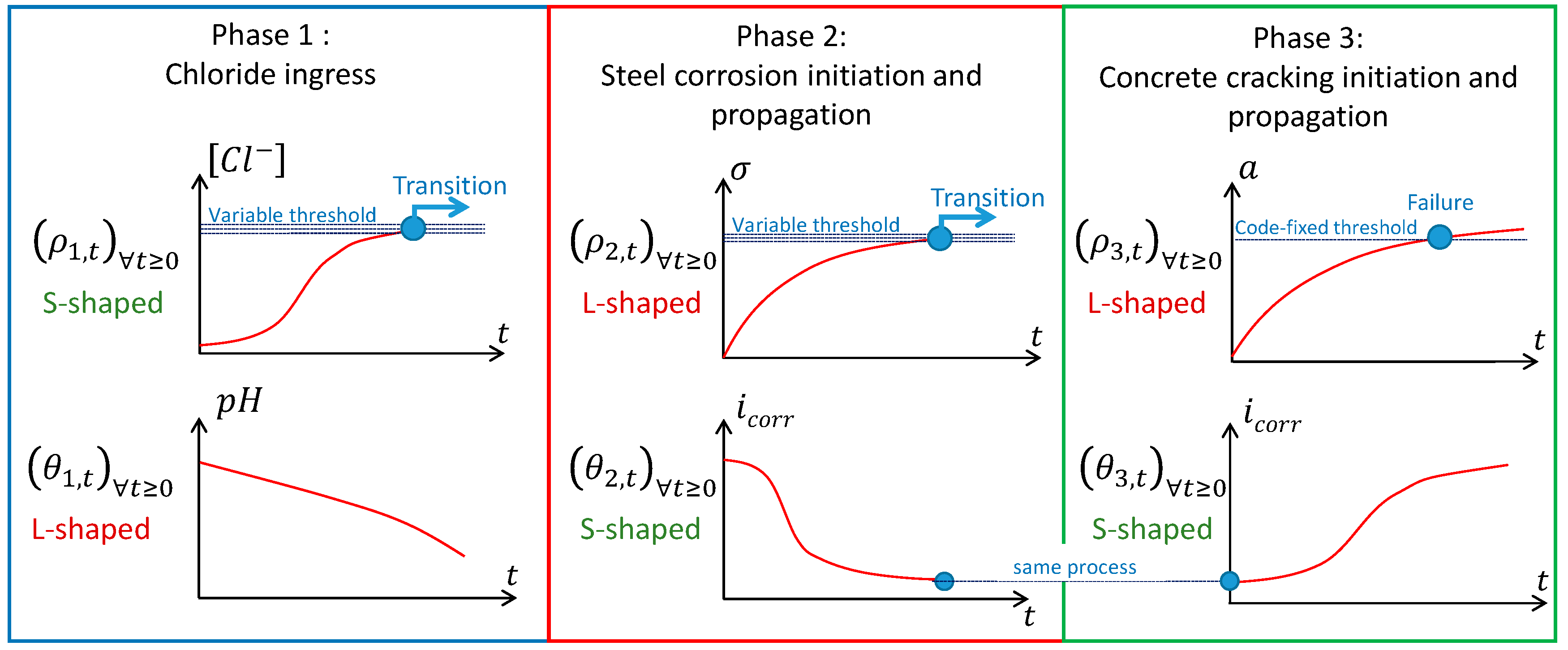
The evolution of the physical indicators over time motivates the choices of each shape function; therefore, we summarize, in
Figure 1, the mean trends of each indicator. These tendencies will dictate the mathematical formulation of the degradation model.
In
Figure 1, we note that the indicators,
,
, and
, share an S-shaped tendency in time. Furthermore,
,
, and
share an L-shaped tendency in time. These shared tendencies simplify the mathematical formulation since it implies similar mathematical expressions for the indicators, as well as similar shapes for identification.
3.3. Mathematical Formulation
The degradation meta-model covers the three phases of chloride-induced cracking of reinforced concrete. This section details the mathematical formulation of the expression constituting the degradation meta-model.
3.3.1. First Phase: Chloride Ingress
As seen earlier, the corrosion initiation phase is characterized by two parameters:
, represents the concentration of chloride at the surface of the steel ;
, models the basicity of the concrete .
To model the dependencies, the cause–effect analysis indicates that in a first step we characterize the evolution in terms of changes in
(
), before performing the same for the
(
). The diffusion of chlorides in the concrete matrix can cause the decrease in
(
). The
process has an S-shaped tendency, and the
process has an L-shaped tendency (
Figure 1). As a result, we propose
:
The appropriate shape functions for the S-shaped
and the L-shaped
are:
The sign in Equation (2), in fact the concrete’s , is represented here by , and has a monotonically decreasing evolution. Hence, the function is a truncated gamma probability density function ensuring a non-negative by truncating all possible simulated increments that are bigger than .
3.3.2. Second Phase: Steel Corrosion Initiation and Propagation
Two parameters characterize the steel corrosion initiation and propagation phase:
, represents the internal tensile stress ;
, models the corrosion current density «» .
To simulate, in a first step, we characterize the evolution in terms of changes in the corrosion current density (
) before performing the same for the stress (
). Furthermore, we see that the
process has an S-shaped tendency, and the
process has an L-shaped one. Therefore, we propose
:
The appropriate shape functions for the S-shaped
and the L-shaped
are:
We notice the
sign in Equation (5) that is used to respect the monotonically decreasing tendency of the corrosion current density represented by
(
Figure 1). In addition, the
function is the truncated gamma probability density function ensuring a non-negative
by truncating all possible increments that are bigger that
.
3.3.3. Third Phase: Concrete Crack Initiation and Propagation
The concrete crack initiation and propagation phase is characterized by [
2]:
, represents the width of the crack ;
, models the corrosion current density .
This model is sequential in the sense that in a first step we seek to characterize the evolution in terms of changes in the corrosion current density (
), before performing the same for the cracking itself (
). The distributions of the increments are, as follows
:
With the suitable shape functions:
3.3.4. Modelling the Transitions between Phases during the Concrete’s Lifetime
In this study, we propose to model transitions between phases by defining a threshold on the condition level indicators (-process). Here, we identify the values of the thresholds. The fact that the -process is correlated with the -process makes the transition indirectly bivariate; however, we might as well question the benefit of directly modelling a bi-variate threshold.
The transition from the first phase to the second phase is governed by the chloride concentration at the surface of the steel [
13]. Once the
reaches, or exceeds, a threshold value
, the corrosion initiates and a transition to the second phase occurs. Angst et al. have shown that the value of the threshold
is heavily uncertain for different types of concrete and environments. Furthermore, it is known that
is affected by the concrete
and
[
13,
47]. However, this relationship is insufficiently understood to be successfully modelled. Therefore, we propose to model
as independent of
. In this model, a variable threshold is considered, and then modelled using a uniform distribution on a pre-defined interval
.
Then, the internal stress on the concrete governs the transition from the second to third phase; the crack starts to propagate after the internal tensile stress exceeds the ultimate tensile strength of the concrete
. In the Eurocode, the value of
is calculated from the value of the ultimate compressive strength (
). Here, we consider a
, and according to the Eurocode [
48],
. Due to material uncertainty, we consider that
will follow a uniform distribution in the interval
.
Finally, failure is defined when the crack width exceeds a pre-defined crack width (). Unlike the first two transitions, has a deterministic value in this model. In fact, according to Table 7.1N from Eurocode 2, for an exposure class XS3 (i.e., the corrosion of the reinforcement induced by the chlorides from sea water) the maximum allowable crack size is 0.3 mm. However, for illustrative purposes, we consider that the performance of the RC structure is modified when the width of a crack is greater or equal than . A detailed structural analysis is required to define this critical size that would vary depending on the structural component.
3.4. Numerical Example and Results
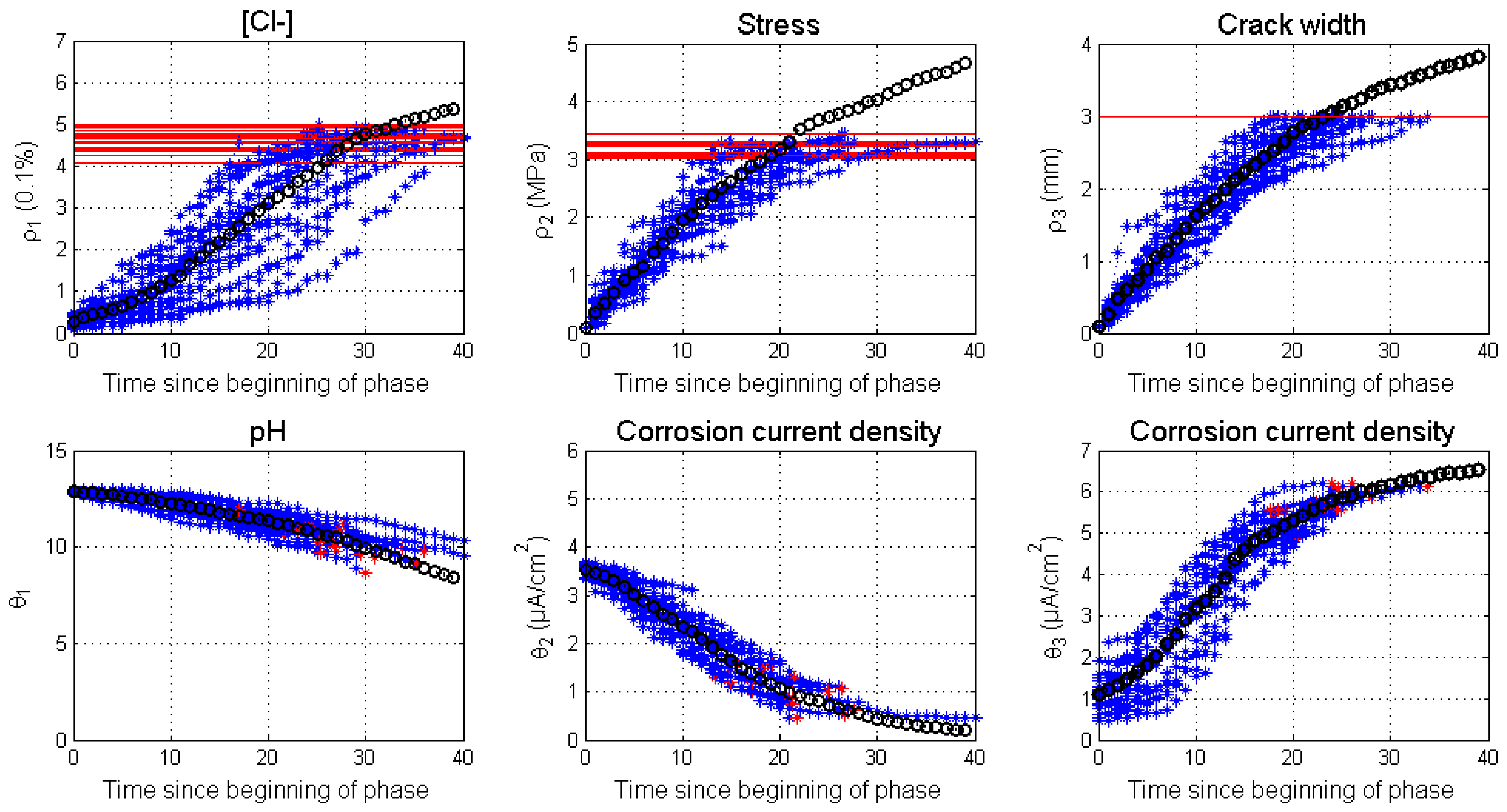
This paper considers the model parameters given in
Table 2. Every parameter can be given a physical meaning, e.g.,
is the abscissa of the point of inflection in the S-shaped tendency of
. Their value is selected according to physical meaning [
2].
Figure 2 illustrates several simulations of the degradation meta-model (blue stars), the mean of these simulations (black circles), the transition thresholds (red lines), and the corresponding values of
for a transition in red stars. We can see the agreement between the simulations and the tendencies of the physical indicators, as presented in
Figure 1.
4. Multiphasic Maintenance Modelling
The aim of this section is to discuss maintenance plans and modelling. First, we catalogue common repair actions applied on corrosion-suffering RC structures. Then, we propose an approach to model the effects of a maintenance action on the model. Finally, we carry out two numerical illustrations to illustrate the use of multiphasic degradation meta-models in maintenance contexts where we consider different maintenance scenarios.
4.1. Repairing Actions Catalogue
The maintenance market disposes of many actions that aim to repair or protect from chloride-induced corrosion damage. These actions aim to re-establish the safety and serviceability structural levels and/or extend its lifetime. The European Standard, EN1504, embraces a performance-based approach (PBA), which is based on the establishment of performance requirements for the repair process, and is evaluated according to recommended conformity tests [
49].
In this study, we consider four of the most common repair methods: concrete replacement, cathodic protection, hydrophobic impregnation, and chloride extraction. The reader may refer to EN1504 for additional details and methods. In addition,
http://durati.lnec.pt (accessed on 1 December 2022) offers a detailed technical guide on inspection and maintenance methods.
4.1.1. Concrete Replacement
Concrete replacement (
CR) restores the original concrete condition by replacing the highly contaminated concrete [
50]. In the case of chloride-induced corrosion, we can apply concrete replacement at three different levels, respectively, to the three phases:
Level 1 []: A preventive action aiming to repair before the corrosion initiation by replacing a few centimetres of chloride-contaminated concrete (before the cover depth);
Level 2 []: A corrective action where limited steel loss occurred, and is characterized by the cleaning of the corroded area to allow an adhesion between steel and the new concrete;
Level 3 []: A corrective action taking place after severe concrete cracking due to a significant loss of the cross-sectional area. Corroded bars are replaced. Substantial costs are added due to the stopping of the structure productivity.
For [] and [], concrete covers are repaired by removing about 6 cm of material for the slabs and beams: 5 cm of cover and 1 cm to clean the rebar.
4.1.2. Cathodic Protection
Cathodic protection (CP) is an electrochemical technique used to control corrosion. systems protect the metal reinforcement bars in the concrete from corrosion and also, in some cases, prevents cracking. converts the active anodic sites on the reinforcement surface to passive cathodic sites by supplying an electrical current or through free electrons from an alternate source. Generally, we achieve via two ways: applying an impressed DC current from an electrical source, or using galvanic action, which is also known as sacrificial anodes.
4.1.3. Hydrophobic Impregnation
Hydrophobic impregnation (HI) processes aim to prevent the ingress of water and aggressive substances that are associated with various degradation processes, in this case chlorides. The treatment by hydrophobic impregnation involves the application of low viscosity water-repellent liquid products, such as silanes and siloxanes on the surface of the concrete.
is applied to new structures, i.e., before the initiation of the deterioration processes, or is included as part of a repair system. If the deterioration process reaches a damage state in the concrete, the application of this treatment requires repairing via a concrete replacement before starting
(see
Section 4.1.1). The treatment is not effective where deterioration has already taken place.
4.1.4. Chloride Extraction
Chloride extraction (CE), sometimes called desalination, is an electrochemical process to remove chloride ions from a chloride-contaminated concrete through ion migration. An anode embedded in an electrolyte medium is temporarily applied on the surface of the concrete, forcing the to migrate outside the concrete. The effectiveness of remains questioned; however, for illustration purposes, it is interesting to consider it since is a specific action related to the first indicator of the first phase, i.e., ).
4.2. Effect of Maintenance Actions on the Meta-Model
The ability to model the effect of a maintenance action on the degradation model is essential for a degradation prediction model, especially with respect to being able to consider imperfect maintenance actions where the system is not restored to one that is as good as new. A maintenance action can have two effects on the degradation process: on the speed of evolution (e.g., decelerates the corrosion processes); and on the current level of degradation (e.g., removes certain quantities of chlorides inside the concrete).
We propose to model the effect of a maintenance action on the speed of evolution directly in the shape functions by introducing a new parameter for each phase:
, where
is the phase number [
51]. For an “S-shaped” trend, the effects of a maintenance action on the shape function are modelled as follows:
where
reflects an acceleration or deceleration ratio, as follows: if
, the process accelerates; if
, then the maintenance action has no effect; and if
, then it decelerates.
By modelling the effect of maintenance through using self-explanatory parameters, we benefit in two ways: (1) the identification of allows one to quantify the effect of a maintenance action; and (2) it is practical to compare the effects of different maintenance actions.
Some maintenance actions can reduce the current degradation level to a post-maintenance degradation level. This post-maintenance degradation level is subject to a high level of uncertainty due to the difficulty in its measurement. Furthermore, it is highly related to internal and external conditions, such as the efficiency and the quality of the maintenance procedure. We propose to model the post-maintenance degradation level through a uniform random variable that is distributed on an interval.
Table 3 summarizes the effects of the catalogued maintenance actions. In addition, the values of the parameters in this table are based on expert judgment.
4.3. Performance Indexes
In a CBM, the condition or performance of the structure are the basis of the decisions. In order to describe the performance of a structure, we find, in the literature, different types of performance indicators [
33]. The most common ones are reliability indexes [
52,
53], safety indexes [
54], and condition indexes that are based on the value of inspection [
55] and are widely used for bridge management [
56].
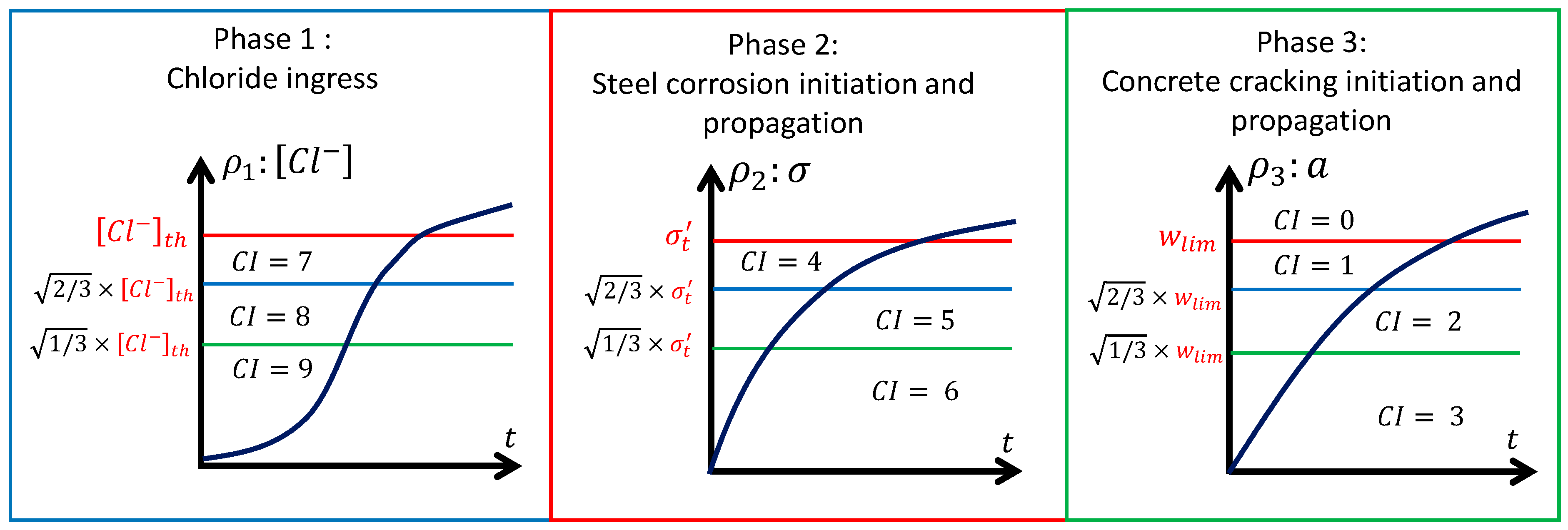
In this study, we consider a condition indexing (
) approach. We classify the condition of the structure in 10 classes. Three classes per phase and one final class for failure, starting from a
, which is associated with a low concentration of chlorides. If it comes down to
, this is associated with failure. We propose to define the
classes based on the value of the
process only (i.e., chloride content, stress, and concrete crack width). The region between the horizontal axis and the threshold line are discretised in three uneven regions through using square root intervals [
57].
Figure 3 summarises the discretisation of the three phases into 10 classes. It is important to note that in phases 1 and 2 the transition thresholds are probabilistic (see
Section 3). Consequently, the underlying
intervals, which are defined based on these thresholds are indirectly probabilistic.
In this study, we aim to illustrate the use of the model, not to optimise the number and length of the
classes. However, we can suggest an optimisation procedure based on an analysis of a Markov decision process in a dynamic context, such as the policy iteration algorithm [
58,
59].
Appendix A provides the flowcharts for the whole decision process.
5. Illustrations in a Lifecycle Management Context
This section illustrates the use of the multiphasic degradation meta-model in a lifecycle management context. The main objective of this section is to demonstrate the ability of the proposed approach to model deterioration processes, as well as modelling single-action and multi-actions maintenance policies. Towards this aim, we first propose to illustrate how to model a deterioration process that could be equivalent to an unmaintained maintenance policy (
Section 5.1). Then, we focus on modelling and comparing two single-action maintenance policies in terms of costs and performances for different target lifetimes (
Section 5.2). Last, we focus on modelling and quantifying the benefit of multi-action policies in an open time horizon context (
Section 5.3).
In these studies, inspections are considered perfect and simultaneous with decisions. This is justified by the fact that we consider monitoring-based inspection [
42] for which a filter can be used for [
60]. The inter-inspection times and the inspection planning for the maintenance policies are later defined in each plan description.
Table 4 summarizes the maintenance and inspection costs for all repair actions. Concrete replacement
costs are defined from a recent and real repair of a marine harbour in Saint-Nazaire, France [
61]. For the remainder of the table the values are estimated, as based on expert judgement.
5.1. Modelling the Deterioration Processes (Unmaintained Maintenance Policy)
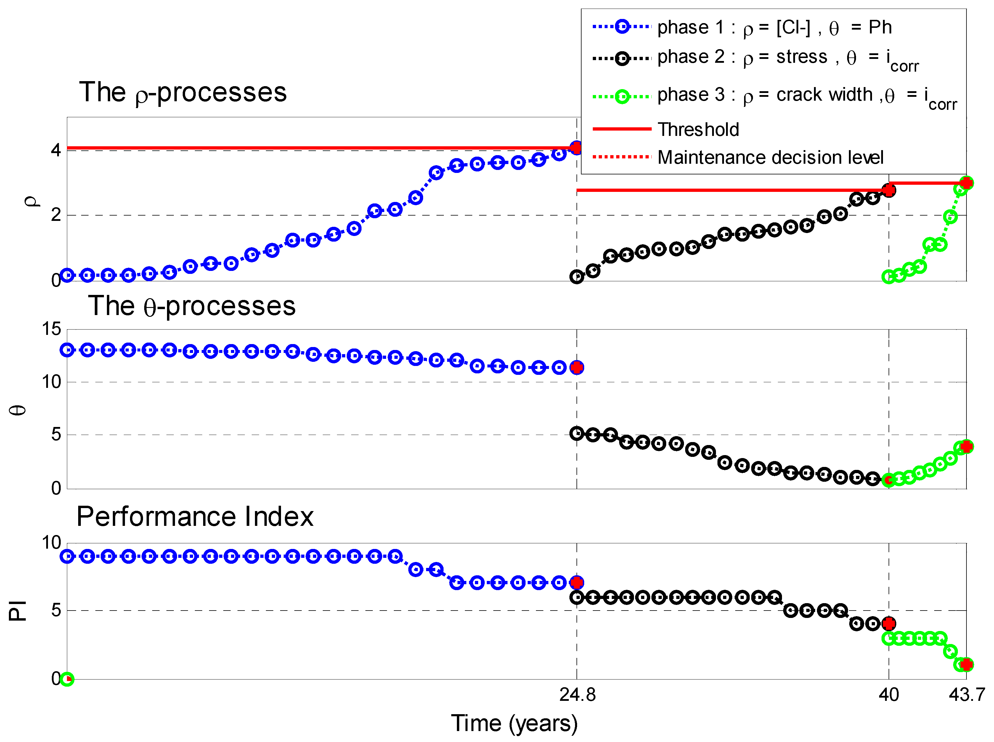
Let S0 be the scenario outlining the deterioration processes (unmaintained structure) where we monitor the six physical indicators every year, but do not carry out any maintenance action. This case serves as a reference scenario.
Figure 4 illustrates one realisation of the S0 scenario.
Figure 4 consists of three plots regarding one realization of each process: (1) the top plot represents the
indicators per phase (chloride content, as well as stress and crack width) and controls the transition between the phases (red line); (2) the second plot shows the
indicators per phase (
and corrosion current density); and (3) the bottom plot tracks the evolution of the performance index (here, the condition index is
) in time. The
indicators show that corrosion starts at 24.8 years, concrete cracking starts at 40 years, and the threshold crack is reached at 43.7 years. It is obvious that if any maintenance action is performed, then the performance index will decrease with time.
5.2. Single-Action Maintenance Policies
5.2.1. Preventive Maintenance Policy
The Preventive Maintenance (
PM) policy aims to prevent the steel initiation of corrosion by applying a
before the transition into the second phase (
). This results in conserving the steel and keeping it intact. The inter-inspection period is set at 5 years [
4,
42,
62] and we inspect the steel for the indicators of the actual period (e.g., if it is estimated we are in the first phase, then the inspections are carried out for
and
).
We discuss the possibility of missing an inspection in the range for this policy. Consequently, this results in not triggering This is due to two reasons: (a) the inter-inspection time is long, and (b) the size of the class is narrow. In this case, inspections for the second phase are required and in order to assess the extent of damage, i.e., to make sure that the corrosion has started. Furthermore, a is required instead of the originally planned , thus generating over-costs that are included in the total maintenance costs of the policy.
5.2.2. Corrective Maintenance Policy
The Corrective Maintenance (CM)policy aims to repair the structure after excessive cracking (i.e., the crack width is larger than ) by applying a . In this policy, the inspection plan consists of a 5 year inter-inspection period, where only the crack width is measured. This inspection plan results in a considerable decrease in inspection costs compared to PM.
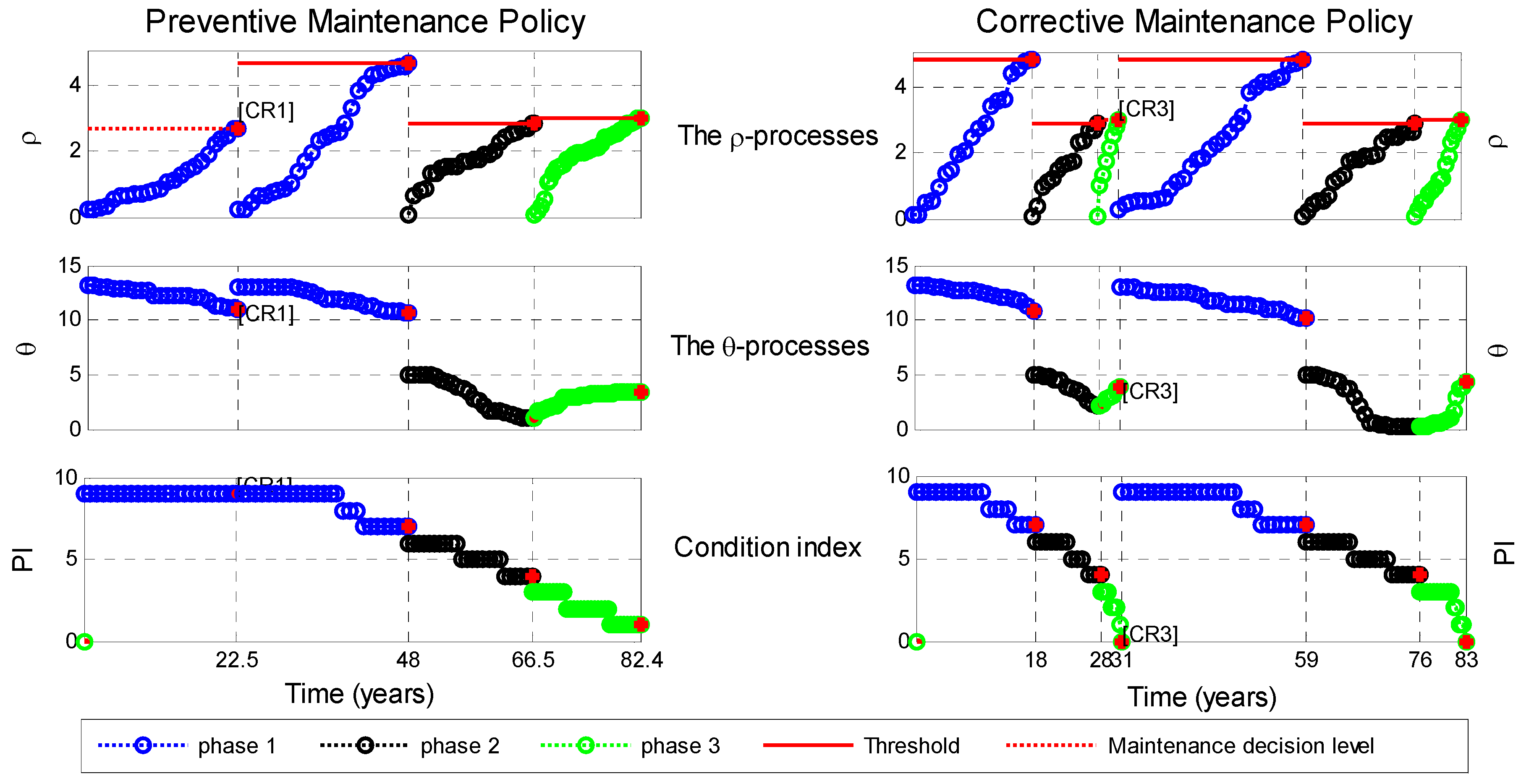
5.2.3. Results: Modelling Single-Action Maintenance Policies
Figure 5 presents a realisation of the application of one preventive and one corrective single-action maintenance action. For the
PM policy, it is noted that
and
become zero after the application of [
CR1] at 22.5 years, thereby delaying the times to corrosion initiation and the severe concrete cracking until 48 and 82.4 years, respectively. For the
CM policy, it is observed that [
CR3] is applied after severe concrete cracking at 61.4 years. Further, the deterioration processes start again until reaching a second severe concrete cracking at 111 years.
These illustrations allow us to see two important trends in terms of : (1) for the PM policy, we notice how the condition index keeps high values in the active part of the policy (i.e., when is triggered), which then starts to decrease until the end of the concrete’s lifetime; (2) on the other hand, the CM policy sweeps all the values before carrying its action. Consequently, the mean values of and are expected to be lower for this policy.
5.2.4. Results: Comparison of the Two Policies
Table 5 summarizes the average estimated costs and
s for the three lifetimes (50, 75, and 100 years) of a structure maintained through
PM and
CM policies. For the annual costs and
we also provide the value of the standard deviation.
Table 5 shows that the
CM policy is cheaper than the
PM policy in terms of inspection costs (
less); however, it is more expensive than the
PM in terms of maintenance action costs (
more), mainly due to the additional expenses associated with the
(
Table 4). Concrete replacement
costs are defined from a recent and real repair of a marine harbour in Saint-Nazaire, France [
61]. For the remainder of the table the values are estimated, as based on expert judgement. In terms of the standard deviation on the estimated total costs
, we notice that the
of the two policies reach their highest values for a required lifetime of 75 years; however, they then decrease softly after that. This observation is explained by the fact that the number of maintenance actions (and therefore total costs) required to fulfil each policy stabilises for a lifetime around 75 years. In terms of annual costs, the values tend to a constant value after 75 years for each policy. However, these results might change if we consider a discount rate.
The results of
Table 5 also indicate that the
CM compromises more than the structural performance, which is expressed as
, in comparison to the
PM. The
PM preserves a higher performance with
for the three lifetimes, while the
CM has a lower mean performance (
). In terms of standard deviation
, we also notice that—similar to
—
leads to a constant value after 75 years for
CM and
PM. However,
is about three times larger for
CM than
PM. This is explained by the fact that
CM allows the structure to sweep over all the
before every
action; consequently, the variability of
increases for this case. In contrast, the
PM policy preserves the structure for a longer period in a
zone, decreasing its
.
5.2.5. Results: The Event of the Missing Corrosion Initiation ( and Its Consequences
The probability of missing
is defined as the probability of having two consecutive inspections where the first inspection finds a
, and the next inspection finds a
, hence missing an inspection in
.
Table 6 summarizes the probability and resulting costs of the missing
.
Over costs represent about of the total cost for the three lifetimes. This cost can be minimised by two methods:
Modifying the ranges of the condition indexes by increasing the size of ;
Decreasing the time period between the inspections (i.e., increasing the inspection rate).
Figure 3 shows that if the interval
was larger (i.e., the lower bound of the interval is reduced) the probability of missing it becomes lower. However, if that range was excessively increased, an early action might be triggered. On the other hand, if one were to decrease the probability of the missing
, the inspection rate is increased; hence, increasing the inspection costs. Another inspection plan can be based on a risk or condition-based inspection approach, where the time of the next inspection is based on the current level of degradation. For example, if we are in a
, we lower the inspection rate to an inspection per year. In this way, we considerably reduce the probability of missing the aimed
and, with it, we decrease the over costs. For such a case, it would be productive to implement and optimize a time variant inspection strategy.
5.3. Multi-Action Maintenance Policies
This section uses the multiphasic degradation meta-model to simulate complex multi-action maintenance scenarios. For this aim, we carry out a set of numerical calculations for the three scenarios that we define later, which we then compare with S0.
In this section, the inspection plan is supposed to be at its highest level, where we inspect the six indicators at every inspection step or through the monitoring result (conducted every year). This choice will have an impact on the inspections cost; however, an emphasis will be placed on the benefit of optimising inspection plans and on allowing us to compare the maintenance costs of these policies.
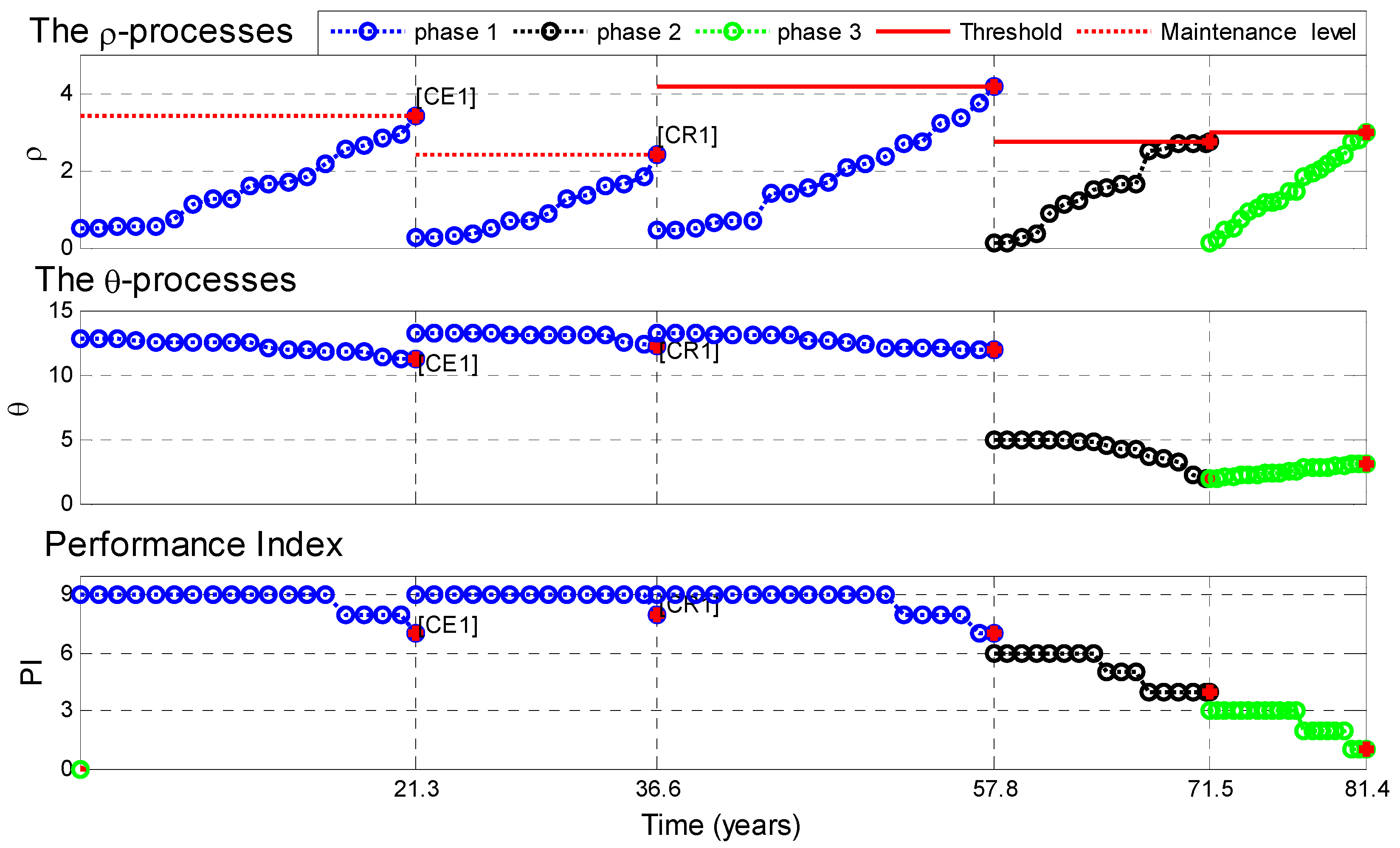
5.3.1. Scenario S1: Apply Once Then, Apply Once
S1 is a preventive maintenance scenario aiming to prevent corrosion initiation.
Figure 6 illustrates one realisation of S1 that exemplifies the multiphasic multivariate and multi-action modelling of degradation and maintenance actions. Its first action is to remove chlorides using
at the end of the first phase (
at 21.3 years).
extracts a high quantity of chlorides and, as a result, restarts the first phase with a remaining quantity of chlorides. Back at
, the chlorides diffuse again in a faster manner due to unremoved chlorides from the previous action. Once
is reached at 36.6 years, a
is carried out to replace the contaminated concrete and extend the lifetime of the structure. It is noted that any maintenance action is performed after
and therefore there is corrosion initiation at 57.8 years and severe concrete cracking at 81.4 years.
5.3.2. Scenario S2: Apply after Construction, and Then Once
S2 is a corrective maintenance scenario that starts with the application of hydrophobic impregnation . This is conducted at the time of the construction of the structure in order to slow down the ingress of chlorides into the concrete, thus extending the lifetime of the structure. S2 also aims to intervene on the structure once by replacing the concrete and the steel for . In addition, requires the structure not be used, thus generating large direct and indirect costs that are included in the estimated maintenance costs. It should be noted that the risk of structural failure is large when the condition index is close to 1.
5.3.3. Scenario S3: Apply after Construction Then Once and Once
S3 is a maintenance scenario aiming to decrease the corrosion rate and avoid the appearing of concrete cracks. First, an is applied at the time of construction in order to slow down the ingress of chlorides. Then, after the corrosion initiation (), a cathodic protection is actived to slow down the corrosion process and extend the lifetime of the steel. Finally, once the extent of damage approaches the cracking initiation (), the concrete is replaced and the corroded rebars are cleaned .
5.3.4. Results and Discussions
We illustrate these scenarios by estimating the following statistical quantities, as based on 10,000 stochastic-based simulations:
(years): Mean lifetime under the considered scenario;
, Probability of a lifetime under 50 years and over 75 years, respectively. These probabilities can be considered as the criteria of optimisation regarding decision;
: Mean condition index during the whole lifetime;
, : Mean total cost of the maintenance actions and inspections, respectively;
: Mean total cost of the scenario = ;
: Mean maintenance-cost-to-lifetime ratio.
Unlike the study that is presented in the previous section, the time horizon is not fixed to 50, 75, or 100 years since it remains a subjective choice—in other words, an open time horizon is used in this study.
Table 7 summarizes the estimated statistical quantities for these scenarios. It is observed that an increase in the performance and lifetime (
and
) of the structure occurs for the three maintenance scenarios, when in comparison to S0, but with a larger lifetime for S3. The preventive scenario S1 has the highest
while having the lowest expected lifetime between the maintained scenarios. This is because S1 extends the period where the structures have higher
CI but a single
[CR1] does not extend the lifetime significantly. The results show that S2 has the highest total costs, 300 more than S3 and almost double S1. However, total costs consider the same inspection costs that depend on the total lifetime and that which could be reduced for each scenario. For example, for S1, an optimised inspection strategy should focus mainly on the parameters of the phase and consider the different inspection lengths. Consequently, if inspection costs are discarded,
Table 7 also presents the ratio between
, which represents an annual maintenance cost. This ratio indicates that the average annual cost of S1 is significantly lower than the costs of S2 and S3.
6. Conclusions and Perspectives
In this paper, an approach to develop multiphasic models of pathologies in a lifecycle management context was proposed. The proposed approach combines the main advantages of the probabilistic models (i.e., the accessibility to NDT and to uncertainty), and the physics-based model (i.e., a physical meaning). This combination resulted in data-driven models that could be very useful for the condition assessment of monitored RC structures. Herein, we selected the methodology to apply to a RC structure that was subjected to chloride-induced corrosion, as well as how to model it by using a three-phase degradation meta-model. Every phase was modelled using a correlated bivariate state dependent meta-model (gamma process), thus representing two physical indicators that were inspectable through an NDT (including visual inspections) or SHM.
To illustrate the versatility of the model when considering maintenance, different maintenance actions were modelled. The efficient computational requirements of the approach allowed us to illustrate the different maintenance scenarios consisting of single and multiple actions, for both fixed (50, 75, and 100 years) and open time horizons, where the managerial quantities (such as lifetime expectation, total costs, and performance indexes) were estimated. The estimation of these quantities was performed via using Monte Carlo simulations.
The results of this study exemplify the versatility of the degradation meta-model in terms of lifecycle management and degradation modelling. Furthermore, it allowed us to evaluate the benefit of using multiphasic approaches to degradation and maintenance modelling by offering the opportunity to define complex maintenance scenarios, as well as to compare them and to perform technical, practical, and economical discussions based on their findings.
This study can lead to multi objective lifecycle optimisation processes, in terms of inspection and maintenance actions, by using criteria such as costs and performance indexes. Furthermore, the calibration of the model from real databases, the benefit of using non-homogeneous databases, and the uncertainty of measurements are also interesting challenges that need to be addressed to allow the implementation of degradation meta-models in real lifecycle management applications.
Author Contributions
Conceptualization, B.E.H., B.C., F.S. and E.B.-A.; methodology, B.E.H., B.C., F.S. and E.B.-A.; software, B.E.H.; validation, B.E.H., B.C., F.S. and E.B.-A.; formal analysis, B.E.H., B.C., F.S. and E.B.-A.; investigation, B.E.H., B.C., F.S. and E.B.-A.; resources, B.C. and F.S.; data curation, B.E.H.; writing—original draft preparation, B.E.H.; writing—review and editing, B.E.H., B.C., F.S. and E.B.-A.; visualization, B.E.H.; supervision, B.C. and F.S.; project administration, B.C. and F.S.; funding acquisition, B.C. and F.S. All authors have read and agreed to the published version of the manuscript.
Funding
This work is a part of the SI3M project (the 2012–2016 Identification of Meta-Model for Maintenance Strategies), funded by Region Pays de la Loire (France).
Data Availability Statement
The data that support the findings of this study are available upon reasonable request.
Conflicts of Interest
The authors declare no conflict of interest.
Appendix A
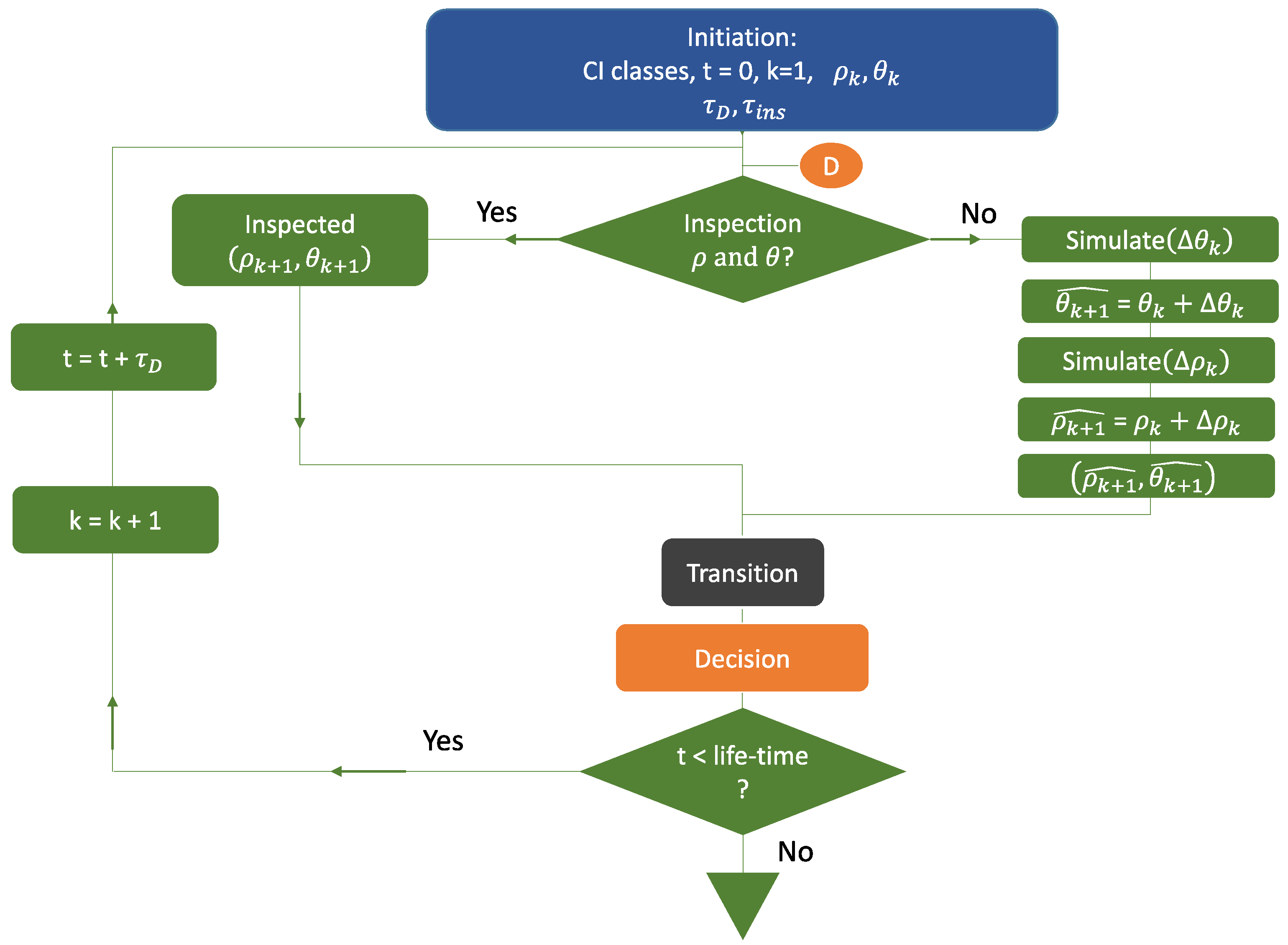
In
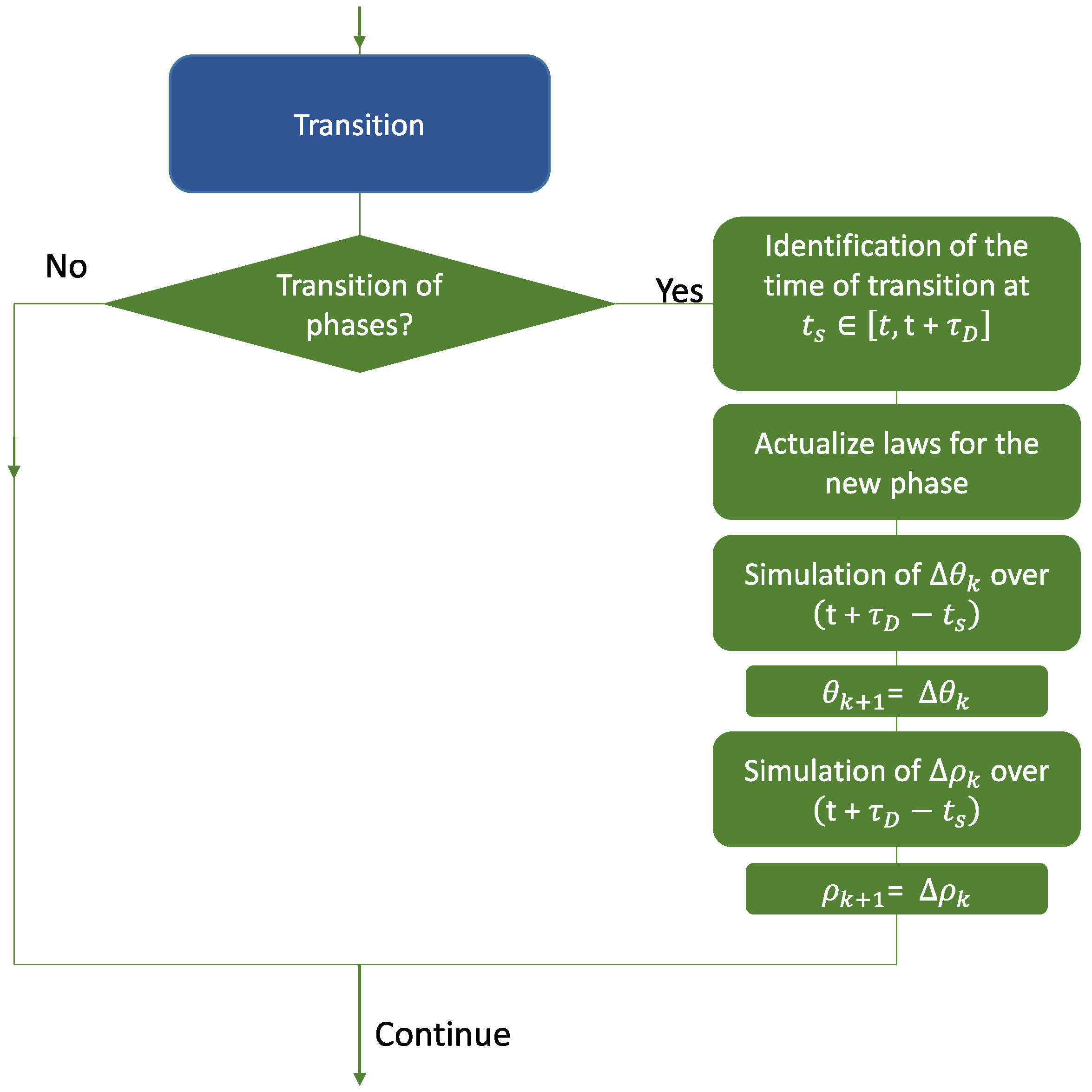
Figure A1, the proposed flowchart for the whole proposed model is summarized. For each time step, the algorithm considers if the structure is inspected or not. The deterioration extent is simulated if the structure is not inspected. Contrarily, the deterioration extent is updated with inspection data. Afterwards, there is a transition step that is detailed in
Figure A2. This transition aims at determining in which deterioration phase the structure is (i.e., chloride ingress, corrosion propagation, or concrete crack growing). If transition occurs, the appropriate laws of deterioration evolution are considered. Once the deterioration phase and its corresponding deterioration extent have been determined,
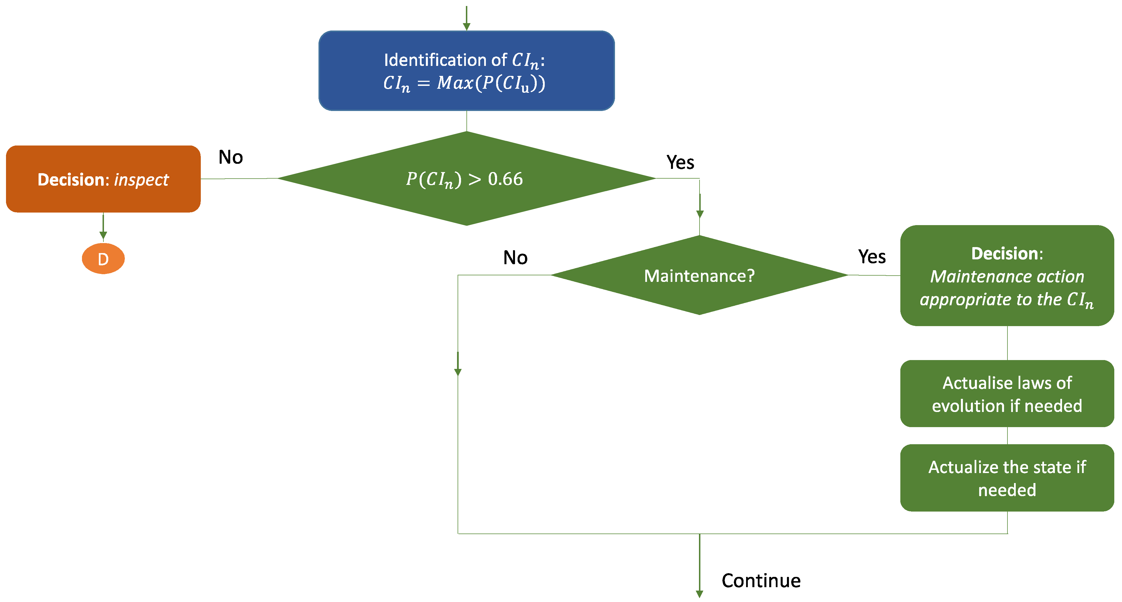
Figure A3 provides the flowchart that integrates the maintenance actions. The aim of this step is to take decisions based on the condition index (
) depending on a threshold probability. In
Figure A3, a probability threshold of 0.66 was selected to initiate the maintenance actions for illustrative purposes. The process is incrementally repeated until the time of the structure reaches the target lifetime.
Figure A1.
General flowchart of the proposed model.
Figure A1.
General flowchart of the proposed model.
Figure A2.
Flowchart of the transition process.
Figure A2.
Flowchart of the transition process.
Figure A3.
Flowchart of the decision process.
Figure A3.
Flowchart of the decision process.
References
- Guo, H.; Dong, Y.; Bastidas-Arteaga, E.; Gu, X.-L. Probabilistic Failure Analysis, Performance Assessment, and Sensitivity Analysis of Corroded Reinforced Concrete Structures. Eng. Fail. Anal. 2021, 124, 105328. [Google Scholar] [CrossRef]
- El Hajj, B.; Schoefs, F.; Castanier, B.; Yeung, T. A Condition-Based Deterioration Model for the Stochastic Dependency of Corrosion Rate and Crack Propagation in Corroded Concrete Structures. Comput. Aided Civ. Infrastruct. Eng. 2016, 32, 18–33. [Google Scholar] [CrossRef] [Green Version]
- Bastidas-Arteaga, E.; Soueidy, C.-P.E.; Amiri, O.; Nguyen, P.T. Polynomial Chaos Expansion for Lifetime Assessment and Sensitivity Analysis of Reinforced Concrete Structures Subjected to Chloride Ingress and Climate Change. Struct. Concr. 2020, 21, 1396–1407. [Google Scholar] [CrossRef]
- Bastidas-Arteaga, E.; Schoefs, F. Stochastic Improvement of Inspection and Maintenance of Corroding Reinforced Concrete Structures Placed in Unsaturated Environments. Eng. Struct. 2012, 41, 50–62. [Google Scholar] [CrossRef] [Green Version]
- Tilly, G. The Durability of Repaired Concrete Structures. IABSE Symp. Rep. 2007, 93, 1–8. [Google Scholar] [CrossRef]
- Zacchei, E.; Bastidas-Arteaga, E. Multifactorial Chloride Ingress Model for Reinforced Concrete Structures Subjected to Unsaturated Conditions. Buildings 2022, 12, 107. [Google Scholar] [CrossRef]
- Bastidas-Arteaga, E. Reliability of Reinforced Concrete Structures Subjected to Corrosion-Fatigue and Climate Change. Int. J. Concr. Struct. Mater. 2018, 12, 10. [Google Scholar] [CrossRef] [Green Version]
- Marquez-Peñaranda, J.F.; Sanchez-Silva, M.; Bastidas-Arteaga, E. Probabilistic Assessment of Biodeterioration Effects on Reinforced Concrete Sewers. Corros. Mater. Degrad. 2022, 3, 333–348. [Google Scholar] [CrossRef]
- Tuutti, K. Corrosion of Steel in Concrete. CBI Res. 1982. [Google Scholar]
- Myers, L.A.; Roque, R.; Ruth, B.E. Mechanisms of Surface-Initiated Longitudinal Wheel Path Cracks in High-Type Bituminous Pavements. In Proceedings of the Asphalt Paving Technology 1998, Boston, MA, USA, 16–18 March 1998; Volume 67. [Google Scholar]
- Liu, Y. Modeling the Time-to-Corrosion Cracking of the Cover Concrete in Chloride Contaminated Reinforced Concrete Structures. Ph.D. Thesis, Faculty of the Virginia Polytechnic Institute and State University, Blacksburg, VA, USA, 1996. [Google Scholar]
- Sheils, E.; O’Connor, A.; Breysse, D.; Schoefs, F.; Yotte, S. Development of a Two-Stage Inspection Process for the Assessment of Deteriorating Infrastructure. Reliab. Eng. Syst. Saf. 2010, 95, 182–194. [Google Scholar] [CrossRef] [Green Version]
- Angst, U.; Elsener, B.; Larsen, C.K.; Vennesland, Ø. Critical Chloride Content in Reinforced Concrete—A Review. Cem. Concr. Res. 2009, 39, 1122–1138. [Google Scholar] [CrossRef]
- Mangat, P.S.; Molloy, B.T. Prediction of Long Term Chloride Concentration in Concrete. Mater. Struct. 1994, 27, 338–346. [Google Scholar] [CrossRef]
- Bastidas-Arteaga, E.; Chateauneuf, A.; Sánchez-silva, M.; Bressolette, P.; Schoefs, F. A Comprehensive Probabilistic Model of Chloride Ingress in Unsaturated Concrete. Eng. Struct. 2011, 33, 720–730. [Google Scholar] [CrossRef] [Green Version]
- Bazant, Z.P. Physical Model for Steel Corrosion in Concrete Sea Structures—Theory.Pdf. J. Struct. Div. Proc. Am. Soc. Civ. Eng. 1979, 105, 1137–1153. [Google Scholar]
- Liu, Y.; Weyers, R.E.R. Modeling the Time-to-Corrosion Cracking in Chloride Contaminated Reinforced Concrete Structures. ACI Mater. J. 1998, 95, 675–680. [Google Scholar]
- El Maaddawy, T.; Soudki, K. A Model for Prediction of Time from Corrosion Initiation to Corrosion Cracking. Cem. Concr. Compos. 2007, 29, 168–175. [Google Scholar] [CrossRef]
- Reale, T.; O’Connor, A. A Review and Comparative Analysis of Corrosion-Induced Time to First Crack Models. Constr. Build. Mater. 2012, 36, 475–483. [Google Scholar] [CrossRef]
- Nicolai, R.P.; Dekker, R.; Van Noortwijk, J.M. A Comparison of Models for Measurable Deterioration: An Application to Coatings on Steel Structures. Reliab. Eng. Syst. Saf. 2007, 92, 1635–1650. [Google Scholar] [CrossRef]
- Kobbacy, K.; Fawzi, B.B.; Percy, D.F.; Ascher, H. A Full History Proportional Hazards Model for Preventive Maintenance Scheduling. Qual. Reliab. Eng. Int. 1997, 13, 187–198. [Google Scholar] [CrossRef]
- Si, X.-S.S.; Wang, W.; Hu, C.-H.H.; Zhou, D.-H.H. Remaining Useful Life Estimation—A Review on the Statistical Data Driven Approaches. Eur. J. Oper. Res. 2011, 213, 1–14. [Google Scholar] [CrossRef]
- Dekker, R.; Scarfb, P.A. On the Impact of Optimisation Models in Maintenance Decision Making: The State of the Art. Reliab. Eng. Syst. Saf. 1998, 60, 111–119. [Google Scholar] [CrossRef]
- Frangopol, D.M.; Kallen, M.-J.; Van Noortwijk, J.M.; Van Noortwijk, J.M. Probabilistic Models for Life-Cycle Performance of Deteriorating Structures: Review and Future Directions. Prog. Struct. Eng. Mater. 2004, 6, 197–212. [Google Scholar] [CrossRef]
- Van Noortwijk, J.M. A Survey of the Application of Gamma Processes in Maintenance. Reliab. Eng. Syst. Saf. 2009, 94, 2–21. [Google Scholar] [CrossRef]
- Papakonstantinou, K.G.; Shinozuka, M. Optimum Inspection and Maintenance Policies for Corroded Structures Using Partially Observable Markov Decision Processes and Stochastic, Physically Based Models. Probabilistic Eng. Mech. 2014, 37, 93–108. [Google Scholar] [CrossRef]
- Shafei, B.; Alipour, A.; Shinozuka, M. A Stochastic Computational Framework to Investigate the Initial Stage of Corrosion in Reinforced Concrete Superstructures. Comput. Aided Civ. Infrastruct. Eng. 2013, 28, 482–494. [Google Scholar] [CrossRef]
- Papakonstantinou, K.G.; Shinozuka, M. Probabilistic Model for Steel Corrosion in Reinforced Concrete Structures of Large Dimensions Considering Crack Effects. Eng. Struct. 2013, 57, 306–326. [Google Scholar] [CrossRef]
- Cusson, D.; Lounis, Z.; Daigle, L. Durability Monitoring for Improved Service Life Predictions of Concrete Bridge Decks in Corrosive Environments. Comput. Aided Civ. Infrastruct. Eng. 2011, 26, 524–541. [Google Scholar] [CrossRef] [Green Version]
- Zouch, M.; Yeung, T.; Castanier, B. Optimizing Road Milling and Resurfacing Actions. Ind. Eng. 2011, 226, 156–168. [Google Scholar] [CrossRef] [Green Version]
- Mercier, S.; Pham, H.H. A Preventive Maintenance Policy for a Continuously Monitored System with Correlated Wear Indicators. Eur. J. Oper. Res. 2012, 222, 263–272. [Google Scholar] [CrossRef] [Green Version]
- Wang, H. A Survey of Maintenance Policies of Deteriorating Systems. Eur. J. Oper. Res. 2002, 139, 469–489. [Google Scholar] [CrossRef]
- Frangopol, D.M.; Liu, M. Maintenance and Management of Civil Infrastructure Based on Condition, Safety, Optimization, and Life-Cycle Cost∗. Struct. Infrastruct. Eng. 2007, 3, 29–41. [Google Scholar] [CrossRef]
- Saad, L.; Chateauneuf, A.; Raphael, W.; Faddoul, R. Life-Cycle Cost Optimization of Degraded Reinforced Concrete Bridges Subject to Reliability Constraints. In Proceedings of the Fourth International Conference on Soft Computing Technology in Civil, Structural and Environmental Engineering, Prague, Czech Republic, 1–4 September 2015; Civil-Comp Press: Stirlingshire, UK, 2015; p. Paper 15. [Google Scholar]
- Van Noortwijk, J.M.; Cooke, R.M.; Kok, M. A Bayesian Failure Model Based on Isotropic Deterioration Jan. Eur. J. Oper. Res. 1975, 82, 270–282. [Google Scholar] [CrossRef]
- Singpurwalla, N.D. Survival in Dynamic Environments. Stat. Sci. 1995, 10, 86–103. [Google Scholar] [CrossRef]
- Lawless, J.; Crowder, M. Covariates and Random Effects in a Gamma Process Model with Application to Degradation and Failure. Lifetime Data Anal. 2004, 10, 213–227. [Google Scholar] [CrossRef]
- Paroissin, C.; Salami, A. Hitting Times of a Deterministic or Random Threshold by a Non-Stationary Gamma Process. In Proceedings of the fourth International Conference on Mathematical Methods in Reliability, Moscow, Russia, June 2009. 2p. [Google Scholar]
- Bordes, L.; Paroissin, C.; Salami, A. Combining Gamma and Brownian Processes for Degradation Modeling in Presence of Explanatory Variables. hal-00535812 2010. preprint. [Google Scholar]
- Vatn, J. A State Based Model for Opportunity Based Maintenance. In Proceedings of the 11th International Probabilistic Safety Assessment and Management Conference and the Annual European Safety and Reliability Conference, Helsinky, Finland, 25–29 June 2012; Volume 1, pp. 1–4. [Google Scholar]
- Riahi, H.; Bressolette, P.; Chateauneuf, A. Random Fatigue Crack Growth in Mixed Mode by Stochastic Collocation Method. Eng. Fract. Mech. 2010, 77, 3292–3309. [Google Scholar] [CrossRef]
- Schoefs, F.; Oumouni, M.; Follut, D.; Lecieux, Y.; Gaillard, V.; Lupi, C.; Leduc, D. Added Value of Monitoring for the Maintenance of a Reinforced Concrete Wharf with Spatial Variability of Chloride Content: A Practical Implementation. Struct. Infrastruct. Eng. 2022, 1–13. [Google Scholar] [CrossRef]
- O’Connor, A.; Kenshel, O. Experimental Evaluation of the Scale of Fluctuation for Spatial Variability Modeling of Chloride-Induced Reinforced Concrete Corrosion. J. Bridge Eng. 2013, 18, 3–14. [Google Scholar] [CrossRef] [Green Version]
- Räsänen, V.; Penttala, V. The PH Measurement of Concrete and Smoothing Mortar Using a Concrete Powder Suspension. Cem. Concr. Res. 2004, 34, 813–820. [Google Scholar] [CrossRef]
- Hurley, M.F.; Scully, J.R. Threshold Chloride Concentrations of Selected Corrosion-Resistant Rebar Materials Compared to Carbon Steel. Corrosion 2006, 62, 892–904. [Google Scholar] [CrossRef]
- Li, C.-Q.; Melchers, R.E.; Zheng, J.-J. Analytical Model for Corrosion-Induced Crack Width in Reinforced Concrete Structures. Struct. J. 2006, 103, 479–487. [Google Scholar]
- Erlin, B.; Verbeck, G.J. Corrosion of Metals in Concrete-Needed Research. Spec. Publ. 1975, 49, 39–46. [Google Scholar]
- Eurocode, B.S. EN 1992-2:2005; Eurocode 2: Design of Concrete Structures—Part 2: Concrete Bridges—Design and Detailing Rules. The European Union per Regulation: Brussels, Belgium, 2005; Volume 2.
- Raupach, M. Concrete Repair According to the New European Standard EN 1504. Integr. Oncol. Princ. Pract. 2005, 6. [Google Scholar]
- Truong, Q.C.; El Soueidy, C.-P.; Li, Y.; Bastidas-Arteaga, E. Probability-Based Maintenance Modeling and Planning for Reinforced Concrete Assets Subjected to Chloride Ingress. J. Build. Eng. 2022, 54, 104675. [Google Scholar] [CrossRef]
- El Hajj, B.; Castanier, B.; Schoefs, F.; Yeung, T. A Risk-Oriented Degradation Model for Maintenance of Reinforced Concrete Structure Subjected to Cracking. Proc. Inst. Mech. Eng. Part O J. Risk Reliab. 2016, 230, 521–530. [Google Scholar] [CrossRef] [Green Version]
- Nowak, A.S.; Collins, K.R. Reliability of Structures, 2nd ed.; CRC Press: Boca Raton, FL, USA, 2012; ISBN 0415675758. [Google Scholar]
- Lee, J.O.; Yang, Y.S.; Ruy, W.S. A Comparative Study on Reliability-Index and Target-Performance-Based Probabilistic Structural Design Optimization. Comput. Struct. 2002, 80, 257–269. [Google Scholar] [CrossRef]
- DB12/01. The Assessment of Highway Bridge Structures; Assessment, H.A.S. for B.: London, UK, 2001.
- Gattulli, V.; Chiaramonte, L. Condition Assessment by Visual Inspection for a Bridge Management System. J. Comput. Aided Civ. Infrastruct. Eng. 2005, 20, 95–107. [Google Scholar] [CrossRef]
- Pontis. Pontis, User’s Manual, Release 4.0; Cambridge Systematics, Inc.: Cambridge, MA, USA, 2001. [Google Scholar]
- El Hajj, B.; Castanier, B.; Schoefs, F.; Bastidas-Arteaga, E.; Yeung, T. A Condition-Based Maintenance Policy Based On A Probabilistic Meta-Model In The Case Of Chloride-Induced Corrosion. In Proceedings of the 12th International Conference on Applications of Statistics and Probability in Civil Engineering (ICASP12), Vancouver, BC, Canada, 12–15 July 2015. [Google Scholar]
- Littman, M.L.; Cassandra, A.; Kaelbling, L.P. Learning Policies for Partially Observable Environments: Scaling Up. In Proceedings of the Twelfth International Conference on Machine Learning, Tahoe City, CA, USA, 9–12 July 1995; pp. 1–59. [Google Scholar]
- Littman, M.L. Algorithms for Sequential Decision Making. Ph.D. Thesis, Brown University, Providence, RI, USA, 1996. [Google Scholar]
- Oumouni, M.; Schoefs, F. A Perturbed Markovian Process with State-Dependent Increments and Measurement Uncertainty in Degradation Modeling. Comput. Aided Civ. Infrastruct. Eng. 2021, 36, 978–995. [Google Scholar] [CrossRef]
- Bastidas-Arteaga, E.; Stewart, M.G. Economic Assessment of Climate Adaptation Strategies for Existing Reinforced Concrete Structures Subjected to Chloride-Induced Corrosion. Struct. Infrastruct. Eng. 2016, 12, 432–449. [Google Scholar] [CrossRef] [Green Version]
- Bastidas-Arteaga, E.; Schoefs, F. Sustainable Maintenance and Repair of RC Coastal Structures. Proc. ICE-Marit. Eng. 2015, 168, 162–173. [Google Scholar] [CrossRef] [Green Version]
| Disclaimer/Publisher’s Note: The statements, opinions and data contained in all publications are solely those of the individual author(s) and contributor(s) and not of MDPI and/or the editor(s). MDPI and/or the editor(s) disclaim responsibility for any injury to people or property resulting from any ideas, methods, instructions or products referred to in the content. |
© 2023 by the authors. Licensee MDPI, Basel, Switzerland. This article is an open access article distributed under the terms and conditions of the Creative Commons Attribution (CC BY) license (https://creativecommons.org/licenses/by/4.0/).


