To Expedite Roadway Identification and Damage Assessment in LiDAR 3D Imagery for Disaster Relief Public Assistance

Abstract

Aerial surveys using LiDAR systems can play a vital role in the quantitative assessment of infrastructure damage caused by hurricanes, floods, and other natural disasters. GmAPD LiDAR provides high-resolution 3D point-cloud data which enables the surveyor to take accurate measurements of damages to roads, buildings, communication towers, power lines, etc. Due to the high point cloud density, a very large volume of data is generated during an aerial survey. The data collected during the airborne imaging is post-processed with calibration, geo-registration, and segmentation. Albeit very accurate, extracting useful information from this data is a slow and laborious process. For disaster response, methods of automating this process have spurred the development of simple, fast algorithms that can be used to recognize physical structures from the point-cloud data that can later be assessed for structural damage. In this paper, we describe an efficient algorithm to extract roadways from a massive Lidar data-set to assist the Federal Emergency Management Agency (FEMA) in assessing road conditions as a step toward helping surveyors expedite a quantitative assessment of road damages for providing and distributing public assistance for disaster relief.

1. Introduction

With the increasing frequency and cost associated with disasters such as tornadoes, flooding, and hurricanes, there is a critical need to develop capabilities that are optimized to support the processing, exploitation, and dissemination (PED) needs of an incident or disaster response [1]. Capability development is needed to support civilians and public safety before the disaster, during the immediate response, and over the long-term recovery. Remote sensing technologies, such as traditional two-dimensional optical imagery collected by the Civil Air Patrol (CAP) or three-dimensional light detection and ranging (LiDAR) point clouds are enabling technologies to develop the applications that public safety needs. In particular, LiDAR is a sensing modality that uses photon light reflections to produce three-dimensional point clouds. Due to recent advances in sensing techniques and commercial technology transition, LiDAR is being more integrated into incident and disaster response [2].

Examples of this integration are the deployment of an airborne Geiger-mode Avalanche Photo-diode (Gm-APD) LiDAR to comprehensively map Puerto Rico to support the post-Hurricane Maria recovery efforts in summer 2018 and targeted collections of North and South Carolina to support the Hurricane Florence response efforts in fall 2018. In conjunction with ground-based local field surveys, satellite imagery, and open-source datasets, a highly automated workflow was developed to expedite a post-disaster damage assessment. This paper provides an overview of the development and application of an algorithm to assist in processing LiDAR data to enable remote roadway assessments.

1.1. Literature Review and Prior Art

The Federal Emergency Management Agency (FEMA)required a simple and fast method for extracting actionable information from large sets of LiDAR point cloud data. Accordingly, we prototyped an algorithm to distinguish roads and buildings from the other physical structures of the terrain. Identifying features of interest would reduce the time required to complete remote roadway assessment, as users could focus on precise measurements and minimize often difficult and hazardous measurements at the physical site. The prototyped algorithm, as part of a highly automated workflow, could then improve the quality of measurements and enable FEMA to efficiently expedite the transition from response to recovery. The developed algorithm was built upon many concepts established in the literature.

In [3], Bokyo, Funkhouser overlaid OpenStreetMaps (OSM) data on LiDAR data to locate roads and curb edges. For Puerto Rico, the OSM data was often found to be sparse or inaccurate, rendering this method to be of limited use. Other 2D data from satellite and airborne sensors may also be used as cueing tools, but the resolution and accuracy were inadequate and the imagery often out-of-date. Clode, Rottensteiner have extracted and vectorized roads from LiDAR data using attributes such as intensity and local point density of point clouds near the digital terrain model (DTM) [4,5]. Li, Hu, have described a road extraction method using multiple features and using hierarchical primitive groupings to connect road segments for form networks [6]. Liu, Zhang applied the generalized Hough Transform for road detection [7]. Owens [8] explored the use of LiDAR data to uncover roads and trails hidden under a canopy. White, Dietterick [9] used LiDAR-based DEMs to reveal roads covered by a dense forest canopy.

Zhao and You [10] used flatness and convexity properties of the point clouds to discriminate roads from buildings and trees. Zuo, Quackenbush [11] presented a raster road classification and vectorization method using the Radon Transform. Weinmann [12] described a multi-variate geometrical feature-based classifier that could be used for foliage detection. Blomley, Weinman, et al. [13] analyzed common geometric covariance features and suggested improvements based upon shape distributions of known objects. Niemeyer, Rottensteiner, [14] presented a probabilistic approach for contextual classification of point clouds in urban areas. These methods utilize the geometrical information embedded in LiDAR data.

Clode, Zelniker, et al. [15] used height and intensity attributes of points followed by convolution with a phase-coded disk to estimate the width and centerline of roads.

Péchaud [16] described a method of extracting tubular structures by computing geodesic curves in 4D space to include local orientation and scale. Cesar, Jelinek [17] applied Morlet Wavelets to identify blood vessels of the fundus, which is an interesting approach. These methods have been applied to 2D images.

Many researchers have applied Artificial Intelligence to this problem. Hall [18] postulated that feature selection for supervised classification tasks can be accomplished based on correlation between features. Sarker [19] applied Convolutional Neural Networks for classifications using spatio-contextual information for flood mapping. However, a lack of sufficient training data and the time computation resources needed for the massive dataset are often limiting factors for the practical use of such methods.

1.2. Goal of This Paper

In this paper, we present an approach to identify roads from a combination of LiDAR metadata and embedded signal attributes along with point cloud distributions and geometrical attributes. A key design consideration was speed and computational efficiency to enhance an existing public assistance workflow. This method may be extended to identify other physical structures such as buildings, trees, vehicles, etc. In the future, it will enable the generation of sufficiently large training sets for the use of AI for improved performance in the recognition of physical structures that may then be assessed for damage. The novelty of the method is to construct a filter of weighted attributes of points in massive point cloud data to extract structures of interest for quantitative analysis.

1.3. Organization of the Paper

This paper has been organized as follows:

In Section 2, we present a historical background of the development of Lidar sensors at Lincoln Laboratory and recent hurricane events where FEMA played important roles in disaster relief. In Section 2.2 we described FEMA’s need for rapid identification for roadways in massive Lidar datasets. Section 2.3 outlines the algorithm designed for this purpose.

In Section 3 we discuss the application of this algorithm to Lidar sensor data collected in Puerto Rico. Results from three specific cases are presented to show performance and how some of the practical issues were addressed.

In Section 4 we discuss the results and conclusions and potential for future work.

2. Materials and Methods

Hurricane Maria made landfall on the island of Puerto Rico on the 20 September 2017 as a strong Category 4 storm, resulting in 2975 deaths and $ 90B in damage. Power and cell phone services were lost to over 90% of the island, and half of the residents had no running water. The Federal Emergency Management Agency (FEMA) set up a Joint Recovery Office (JRO) in Guaynabo, south of the capital San Juan, to handle recovery efforts with a focus on infrastructure repairs to roadways and buildings, as well as debris removal. In May of 2018, FEMA contracted MIT Lincoln Laboratory to map the entire island as well as the outer islands of Vieques and Culebra with an airborne LiDAR sensor to reduce the time required to assess the damage. A similar effort was conducted to support the North and South Carolina response to Hurricane Florence in the latter half of 2018. 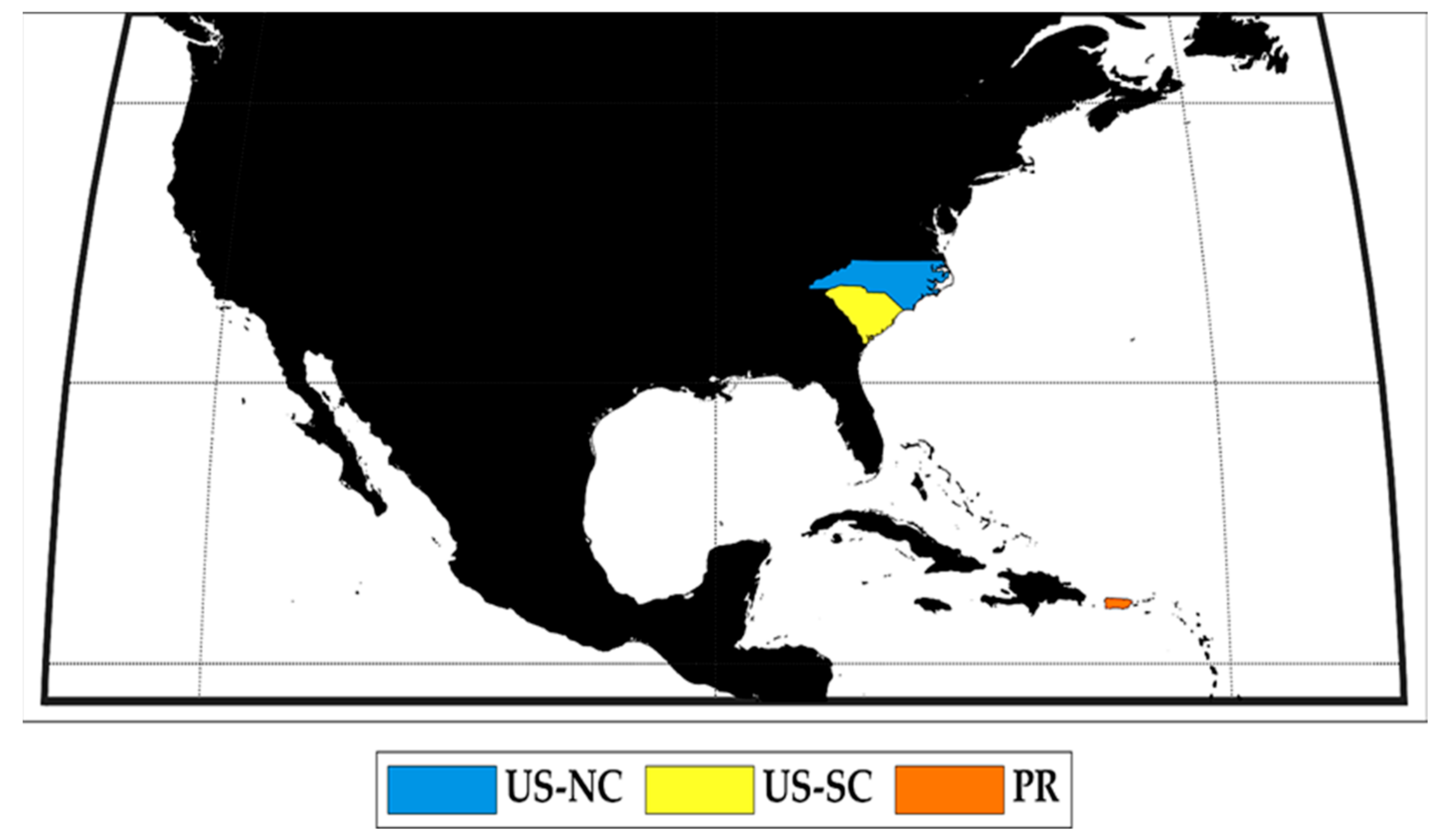Figure 1 shows some of the locations on a map where the airborne LiDAR sensor collected data after major hurricanes.

This section discusses the LiDAR sensor, overviews what a roadway assessment should include, and describes the algorithmic development to assist in automating a roadway assessment.

2.1. Airborne Optical Systems Testbed

LiDAR systems-based Gm-APD technology has been under continuous development since the late 1990s at the MIT Lincoln Laboratory [20,21]. Our work is based on earlier field deployments with iterations of the MIT Lincoln Laboratory Airborne Optical Systems Testbed (AOSTB) and Airborne LiDAR Imaging Research Testbed (ALIRT) systems (Figure 2). The AOSTB is significantly more capable than any commercial system available and can collect wide-area, high-resolution, three-dimensional data sets very rapidly. A key capability of the LiDAR is foliage penetration (FOPEN), which allows sensing through dense canopy layers as single photons reflect off the ground as they pass through the canopy.

Data collection was performed at an operating ground speed of 50–99 m/s and GPS altitude of 2070–2470 m above ground level (AGL), which produces point clouds with a 25 cm post-spacing. Depending on the cloud ceiling, the AOSTB may operate as low as 1000–1220 m AGL. As of December 2018, the reference LiDAR consisted of a 1 Watt, Q-switched, Nd: YAG laser at a wavelength of 1064 nm with a pulse width of approximately 500 ps. A more powerful 3-Watt laser was integrated in the summer of 2019. The electro-optical receiver was a state-of-the-art 256 × 64 pixel, 50-micron-pitch, Gm-APD array optimized for operation at the 1064 nm laser transmitter wavelength. A Kontron CP605 with Intel 4M controlled the scan mirror and an Applanix POS AV V6 was used for direct georeferencing. The LiDAR had a theoretical hourly area collection rate of 1000 km²/h. A COTS Coherent laser source was used with an electro-optical receiver fabricated at MIT/LL. The electronic subsystems read out the Gm-APD data and record the raw data along with sensor and platform state data onto physical disks. The onboard operator interfaces were provided to control and monitor the sensor state, laser operations, and data acquisition and recording.

The AOSTB had a single Gm-APD sensor which produced raw data at a rate of 0.25–0.5 GB/s but other systems employ four Gm-APD sensors, outputting at 1–2 GB/s. The initial transformation from raw data to a noisy point cloud required a similar data rate. Next, point filtering and registration algorithms produced a scan-based point cloud outputting at 0.05–0.15 GB/s for the AOSTB. Additional AOSTB processing results in another order of magnitude reduction. When the data was processed, the point cloud cross resolution could improve from 5 m to 0.25 m. Given the current Gm-APD capabilities and processing algorithms, near real-time end-to-end processing required tens of teraflops of computational power.

The high-resolution LiDAR data covering the entire island of Puerto Rico consisted of over 50 TB of data. The point cloud consisted of over 300 billion points. The data was organized into tiles each covering an area of 500 m × 500 m on the ground. Roughly 40,000 tiles were needed to cover the island of Puerto Rico. Each tile consisted of roughly 4–8 million geo-located points, each with various additional metadata [22,23,24]. Processing hundreds of hours of LiDAR data required days to weeks, depending on the desired product, on an interactive supercomputer. With today’s AOSTB collection and automated processing workflow, collecting and processing a 250 square mile area can be accomplished in under 36 h from aircraft take-off to usable 3D data products. The manual extraction of actionable information from these data products could have taken weeks or months.

2.2. Road Assessments

FEMA needed a capability to assess the damage to roadways infrastructure of the island. For major disasters such as Hurricane Maria or Florence, rapid assessments of thousands of damage-sites of roadways were required. The survey teams were dispatched by a joint field office where communications were often difficult due to downed communications towers and power lines. The surveyors performed damage by taking physical measurements of dimensions of damaged infrastructure. This was time-consuming, less accurate, and sometimes hazardous.

In these circumstances, performance in speed preceded accuracy. A sufficiently good, working solution delivered quickly was more valued compared to a “perfect” solution delivered late. Many of the roads were inaccessible due to physical barriers such as landslides, fallen trees, etc. Several common types of roadway damages include landslides, washouts of the shoulder, damages of road-beds and bridges, failures of pipes/culverts, damaged guard-rails, etc. The damage assessments were used for generating engineering reports to provide scopes of repair work, cost estimates, and disbursements of funds. Specifically, roadway assessments primarily consisted of various measurements of the damage feature and surrounding area:

• Length, depth, width, and material of pavement damage
• Length, depth, width, and material of roadbed damage
• Length, depth, and width of shoulder damage
• Length, diameter/width and height, thickness, and material of damaged pipes/culverts
• Length of damaged guard rail

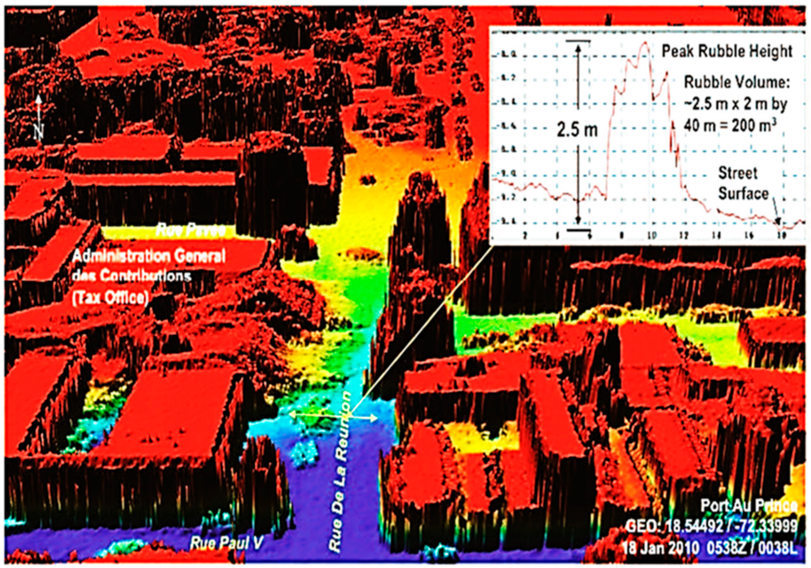
A roadway damage assessment report may contain some or all these features. The assessment may also contain non-measurable information such as affected signage, nearby utilities, roadway route type and name, and information for a local contact. This information was often accompanied by a few sketches, with Figure 3 as an example.

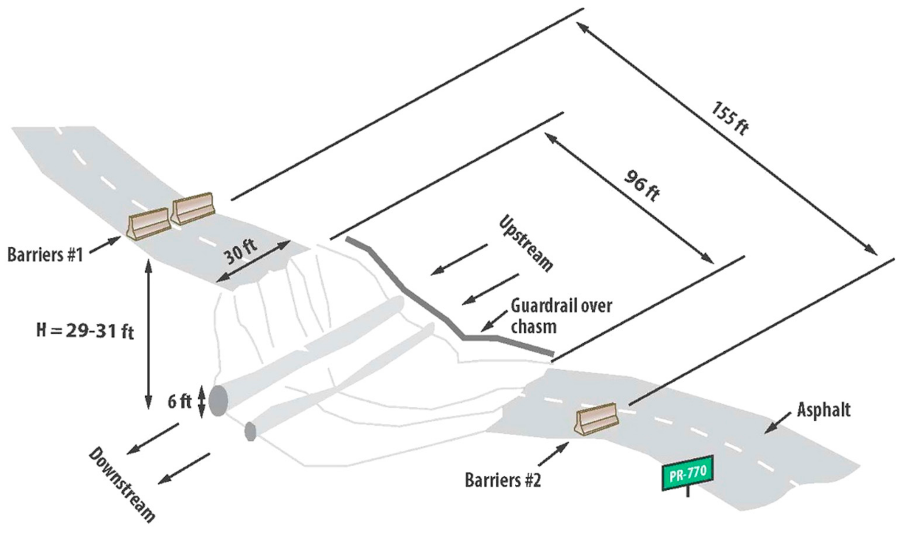
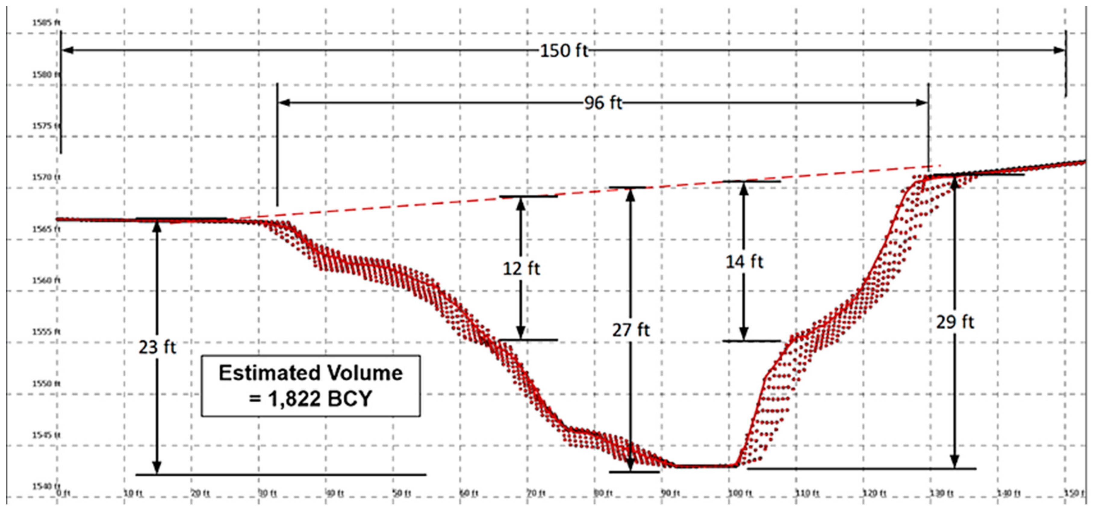
In comparison, Figure 3 shows a damaged section of a road extracted from the LiDAR point cloud that was used to get the desired measurements of the damaged section of the PR-770 near Barranquitas, PR. Here, approximately 100 feet of roadway was washed out in the area passing over Rio Canabon. Roadway assessments primarily consisted of various measurements of the damaged features and the support structures as shown in Figure 4.

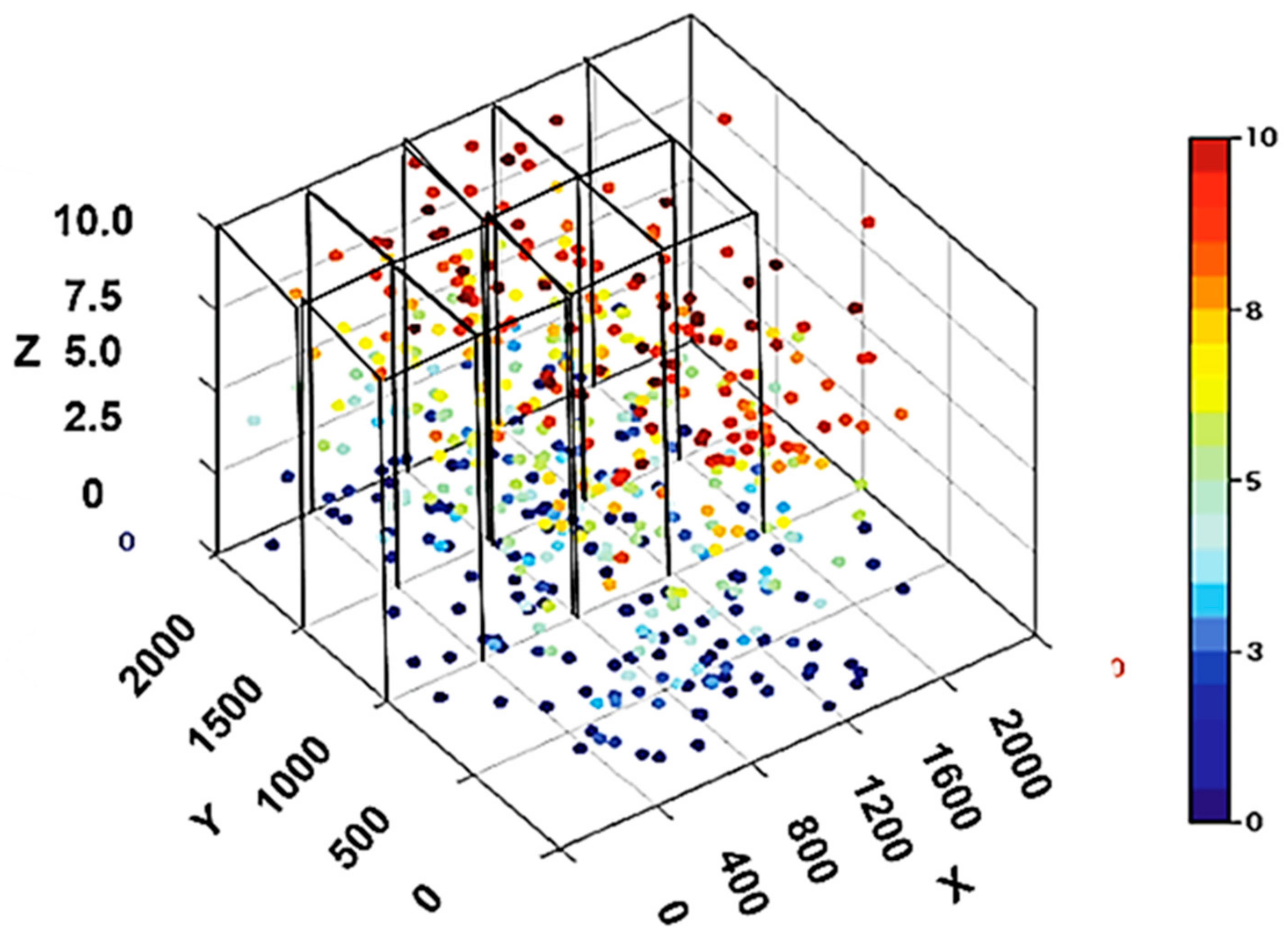
Each red point represents an individual LiDAR measurement. All the features were measured digitally, without the need for a human survey team to hazardously maneuver through the washout.

2.3. Algorithm Design

The approach described here leverages the past work and applies a combination of LiDAR metadata and embedded signal attributes along with point cloud distributions and geometrical attributes. The programming complexity and the computational load of many earlier methods were unfavorable for fast implementation.

To meet FEMA’s requirements, simple, fast algorithms with low computational load were needed. The developed approach was designed to integrate into the existing FEMA public assistance workflow, particularly those established for the Hurricane Maria recovery and Hurricane Florence response. The algorithm’s purpose was to inform and support public assistance workers and assessors. This necessitated a design that effectively utilized the LiDAR signal attributes and metadata.

Furthermore, a key challenge across most incident and disaster research is that while targets of interest, such as roads, are entities that can be discretely annotated, there is an operational need to the quantify damage that is less discrete and lacks clear boundaries. There is a dearth of precise baseline infrastructure measurements that can enable change-detection techniques for damage assessment. This is particularly true for LiDAR-based datasets and hinders any classical machine learning approaches in using change detection as an effective tool for damage assessment. While often after disasters, crowd-sourcing mapping efforts such as the Humanitarian OpenStreetMaps team and Tomnod rely on volunteers to annotate maps, these efforts are often for satellite or optical imagery and not LiDAR. While recognizing this challenge and capability gap, we did not have the resources available to develop an annotated LiDAR dataset. Instead, we adapted an algorithm design methodology that employed basic signal processing approaches.

In response, we prototyped an algorithm designed to leverage the LiDAR metadata and embedded signal attributes including intensity, Height Above Ground (HAG), Signal to Noise Ratio (SNR), and reflectance. The approach was based upon the basic observation that each point of a point cloud by itself provided little useful information about the structure to which it belonged, but when combined with its neighboring points and their attributes, partial features of objects began to emerge. The algorithm divided the data into small sets and used their collective properties to classify them into the corresponding physical structures.

The algorithm leveraged many signal attributes. The intensity, i.e., the recorded amplitude of the reflected pulse captured as a return by the LiDAR receiver (see Appendix A for definitions). LiDAR intensity values can be affected by many factors such as the angle of incidence, target reflectance, and the environment. As a result, they cannot be used as absolute measurements, but their relative magnitude can be used for the classification of points in the LiDAR data set. Target reflectance is the portion of the transmitted energy reflected back by the object to be captured by the LiDAR receiver pertinent. Each object has a unique spectral signature that absorbs, transmits, and reflects the transmitted energy. As a result, they too cannot be used as absolute measurements, but their relative magnitude can be used for the classification of points. SNR is another signal attribute that may be used for classification. To accurately determine the position of each point in object space, the weak optical return signal needs to be detected and its timing measured accurately to within a few nanoseconds. The detection circuit of the GM-APD LiDAR needs to have a high gain, high bandwidth amplifier. This implies a high noise competing with a weak incoming signal. SNR was also used as a distinguishing characteristic to identify features of interest.

These signal attributes were represented as distributions for a given set of three-dimensional positions. There are many ways to represent position using LiDAR measurements and the prototyped algorithm was based on height above ground (HAG) positions. This is the set of last returns (lowest points in the terrain) detected by the receiver. These points were used to generate the bare earth surface. The relative height of each point in the point cloud was measured from this reference surface.

In general, roadways have a HAG with low mean and variance, low SNR, low intensity, and low reflectance. These properties are due to the roadways generally having a uniform, flat surface and are usually at a lower height compared to neighboring structures such as vegetation, buildings, etc. The uniformity of the road surface is represented in the HAG projection. Additionally, the materials of the road surface have low reflectance which provides a low intensity of the return signal from the LiDAR. The diffuse surface also produces a low SNR. In addition, the points on roads will lie in narrow, long contiguous groups of silos except when they are under foliage. These physical attributes were used to identify the road surface using a simple filtering procedure.

The algorithm consisted of the following steps:

• Divide the area of each tile into a grid of small rectangular silos (Figure 5). Each silo will consist of a small base area (e.g., 0.25 m × 0.25 m) and with a maximum height being the highest point in the silo. Assign each point in the silo to one of these silos based upon its geo-location.
• Create a filter based on a moving window of say, a block of 5 × 5 adjacent silos that will pass over the entire tile covering a lawn-mower pattern.
• Create a set of the points in the cloud that fall within this moving window.
• Generate a histogram of each of the attributes of the points in this set (e.g., HAG, Intensity, etc.) Use the properties of the distribution of points and their attributes in each silo to classify them into physical structures (e.g., roads, trees, buildings, etc.).

3. Results

In this section, we present results and discuss the following cases where this algorithm was applied. We have selected 3 example cases that represent the results and some of the advantages and challenges in using the algorithm.

Case 1: Identifying Roads

First, we show how this algorithm was used to identify roads. The attributes of road surfaces described above were exploited to rapidly identify points on roads from dense point clouds containing a variety of physical structures and features.

Case 2: Discriminating Waterways

A practical issue confronted while applying this filter was in distinguishing between roads and waterways since both have very similar physical characteristics as recorded in the LiDAR data. Here we discuss how this problem was addressed by applying a filter for removing the waterways.

Case 3. Identifying Road Under Foliage

Another problem was to extract points in the cloud that are on the road but covered under foliage. During the airborne collection, the LiDAR transmits rays from many directions as it passes over the terrain. As a result, even in the presence of dense foliage, some of the transmitted rays manage to pass through gaps in the foliage and provide a return signal. This sparse set of ‘last returns’ was recovered during post-processing in the HAG data and used to find parts of the roads under foliage to form a continuum with the open, exposed parts of the road. It is possible to recover portions of the road that lie under foliage. In this example, we present a method of finding the road surfaces that are hidden under foliage.

3.1. Case 1 Identifying Roads

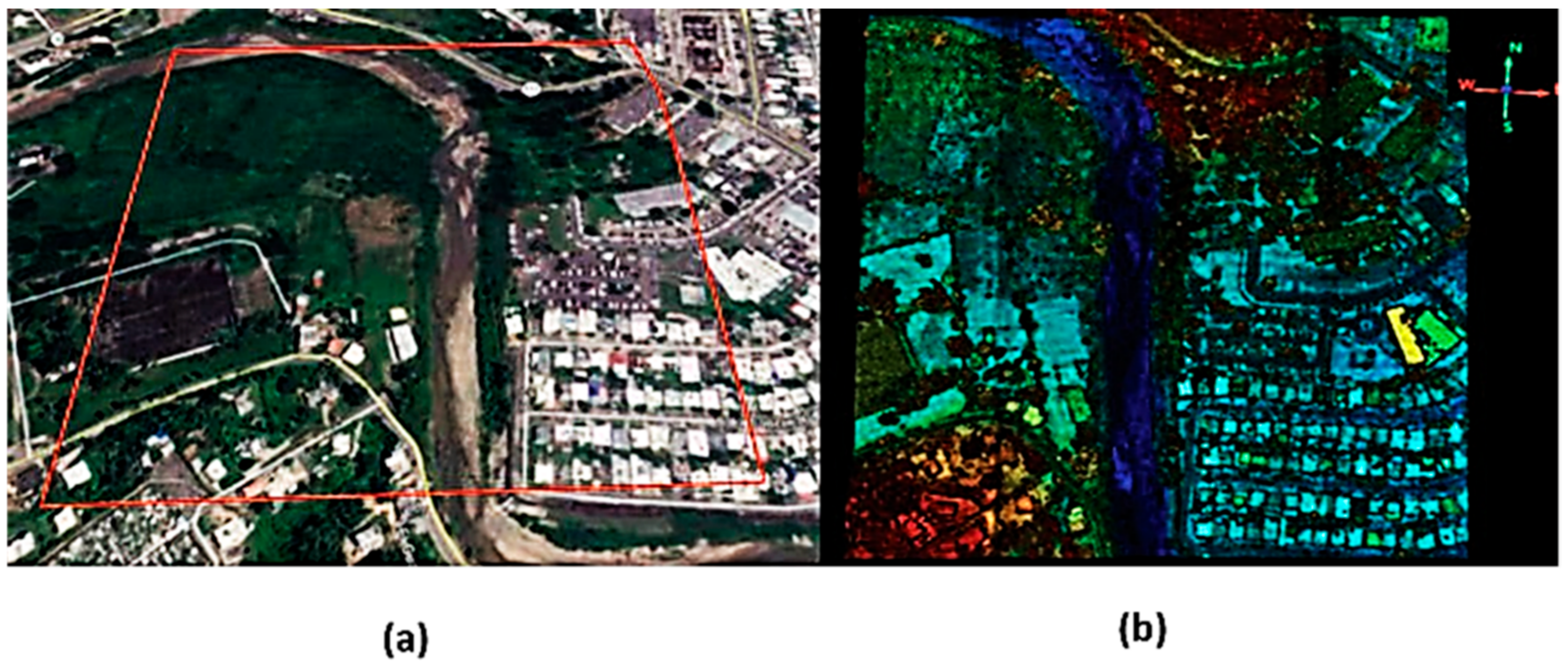
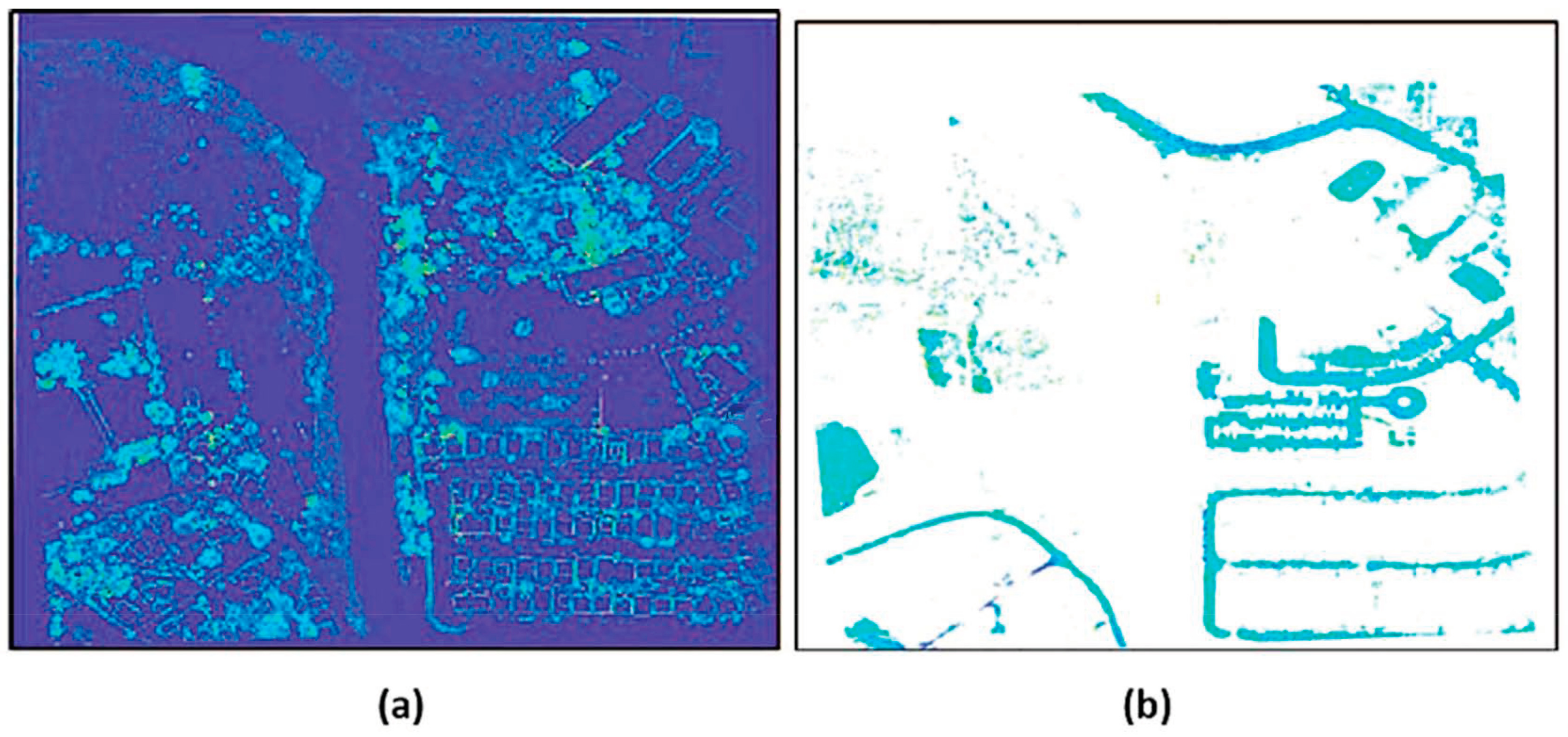
Figure 6 shows a view from Google Earth of an area in Utuado, PR. In the Google Earth image in Figure 6a, the red bounding box shows a 500 m × 500 m area on the ground. Figure 6b shows the corresponding LiDAR image. This area was selected as an example use-case because it includes various types of terrain encompassing a network of roads. This includes urban/settled areas in the southeast part and dense, wooded areas in the northwest. It also has a water canal that flows in the center in the north-south direction. In 2D imagery such as with an EOIR camera, it is easy to spot some of the roads that can be distinguished by their color, shape, and relative size. However, many road segments are difficult to identify because they have colors and shapes that may be confused with other features, or they are hidden under foliage. The LiDAR 3D data gathered during the Puerto Rico campaign made it possible to distinguish roads from similar features by using filters that utilized a combination of meta-data and geometric information encoded therein. On the other hand, the high-density data presented challenges in terms of computation load. Any algorithm developed for finding roads had to be scalable for processing the large volume of data in a reasonable time frame (minutes instead of hours or days). This was driven by FEMA’s need for rapid processing and analysis of the LiDAR data to assist and expedite the disaster relief efforts. The algorithm described above was applied to the LiDAR data. The unfiltered HAG data is shown in Figure 7a and the filtered data after applying the algorithm described above is shown in Figure 7b.

As shown in Figure 7b, most of the roadways were identified quite easily. However, because the roads have similar attributes to parking lots, runways, helipads, etc., these were also included in the filtered data. These other structures are usually easy to identify by their physical shapes and can be removed by post-processing. The processing results are summarized in

Table 1. Case 1 Results Summary.

TILE ID	X329_Y096
Total No of points	4,589,032
Total No of Silos	991 × 1024
No of Silos on Roads	221,886
Avg Pts per Silo	3.9467
Stdev No of All Pts per Silo	0.933
No of Points on Road	383,391
Mean HAG of points on Roads	0.0105
Stdev of HAG of points on Roads	0.1115
Mean HAG of all points	1.7969
Std HAG of all points	3.2337

. About 8.3% of all the points in the cloud were found to be on roads. The ratio of the means of the points on the roads vs all the points in the cloud was 0.005 and the ratio of the standard deviations was 0.034.

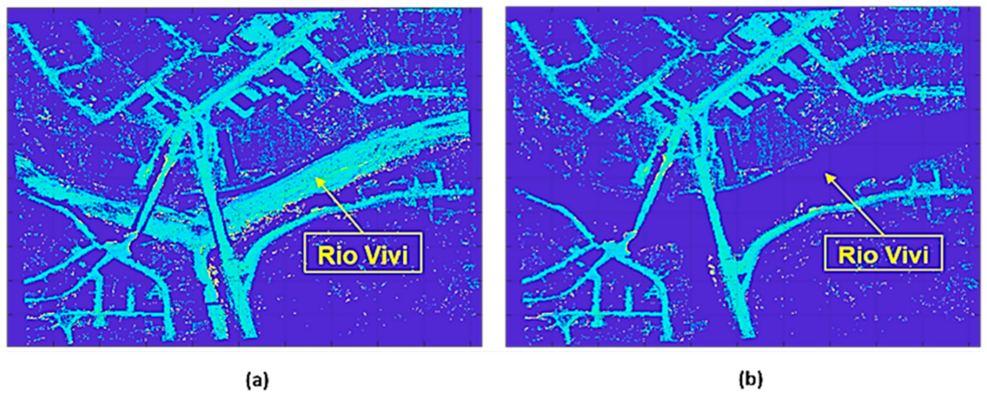
3.2. Case 2 Discriminating Waterways

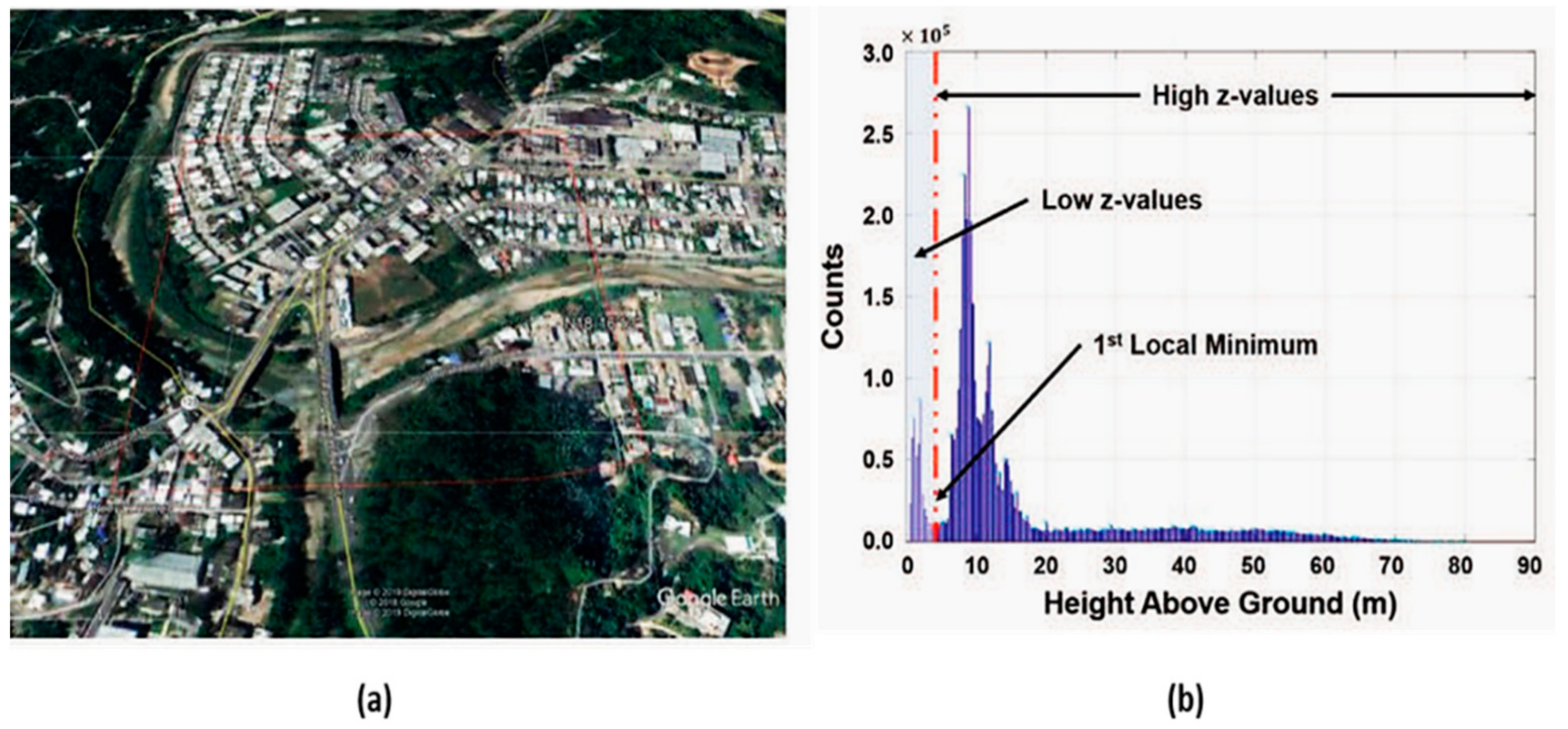
In this use case, we demonstrate a refinement to the algorithm to distinguish roadways from waterways. Like roads, waterways are flat, have low Reflectance and Intensity. The original algorithm was not able to distinguish between roads and waterways. The solution to this problem was found by utilizing traditional civil engineering best practices [1]. In general, the road levels are designed to be above the water levels. To apply this principle the first minima of the histogram of the Z-data of each tile (Figure 8b) was used to separate the low-level and the high-level Z-data points. The low-level data points were removed from the set before the road-finder algorithm was employed. This proved to be an effective method for separating waterways from roadways (Figure 9).

Table 2. Case 2 Results Summary.

TILE ID	X328-096
Total No of points	4,669,733
Total No of Silos	992 × 1000
No of Silos on Roads	195,894
No of Points on Road	391,400
No. of Points on Waterbodies	428,585

is a summary of the results for this use case. There were roughly 4.7 million points in the point cloud representing this tile of which roughly 8.3% were found to be on roads and about 9.8% were on water bodies.

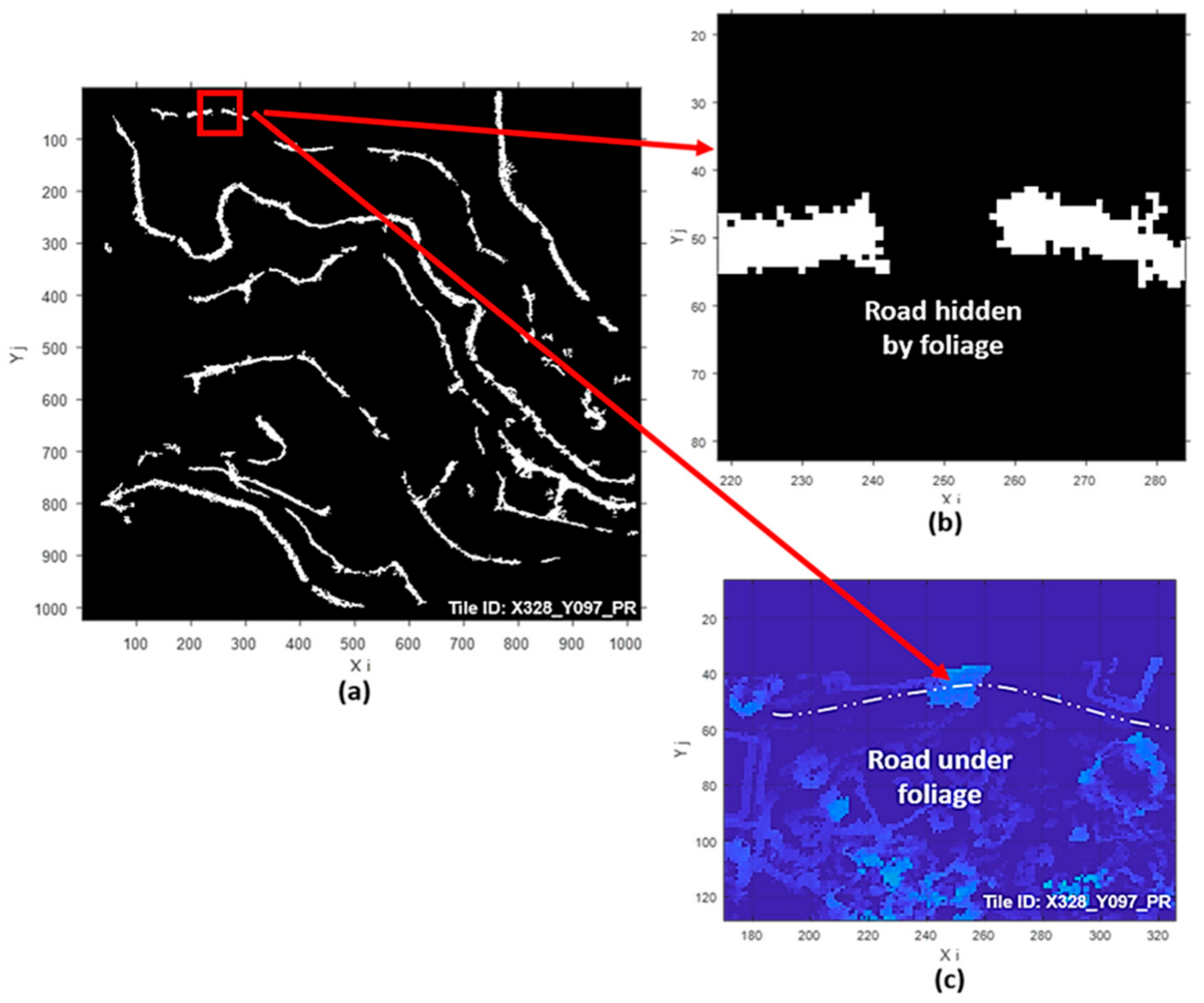
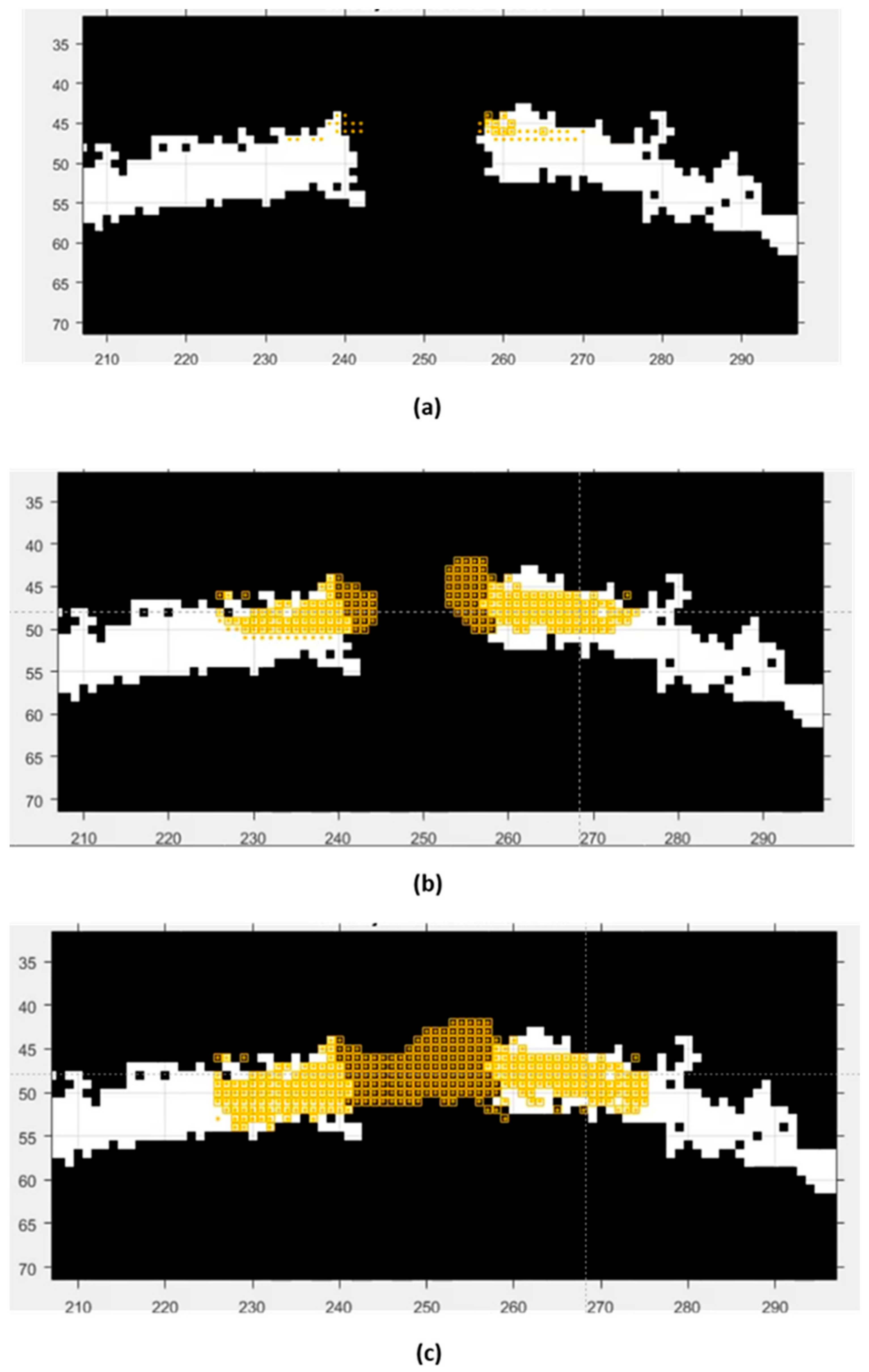
3.3. Case 3 Identifying Roads under Foliage

The next problem was to extract points in the cloud that are on the road but covered under foliage (Figure 10). In this example, we show how the problem of finding roads hidden under foliage was addressed.

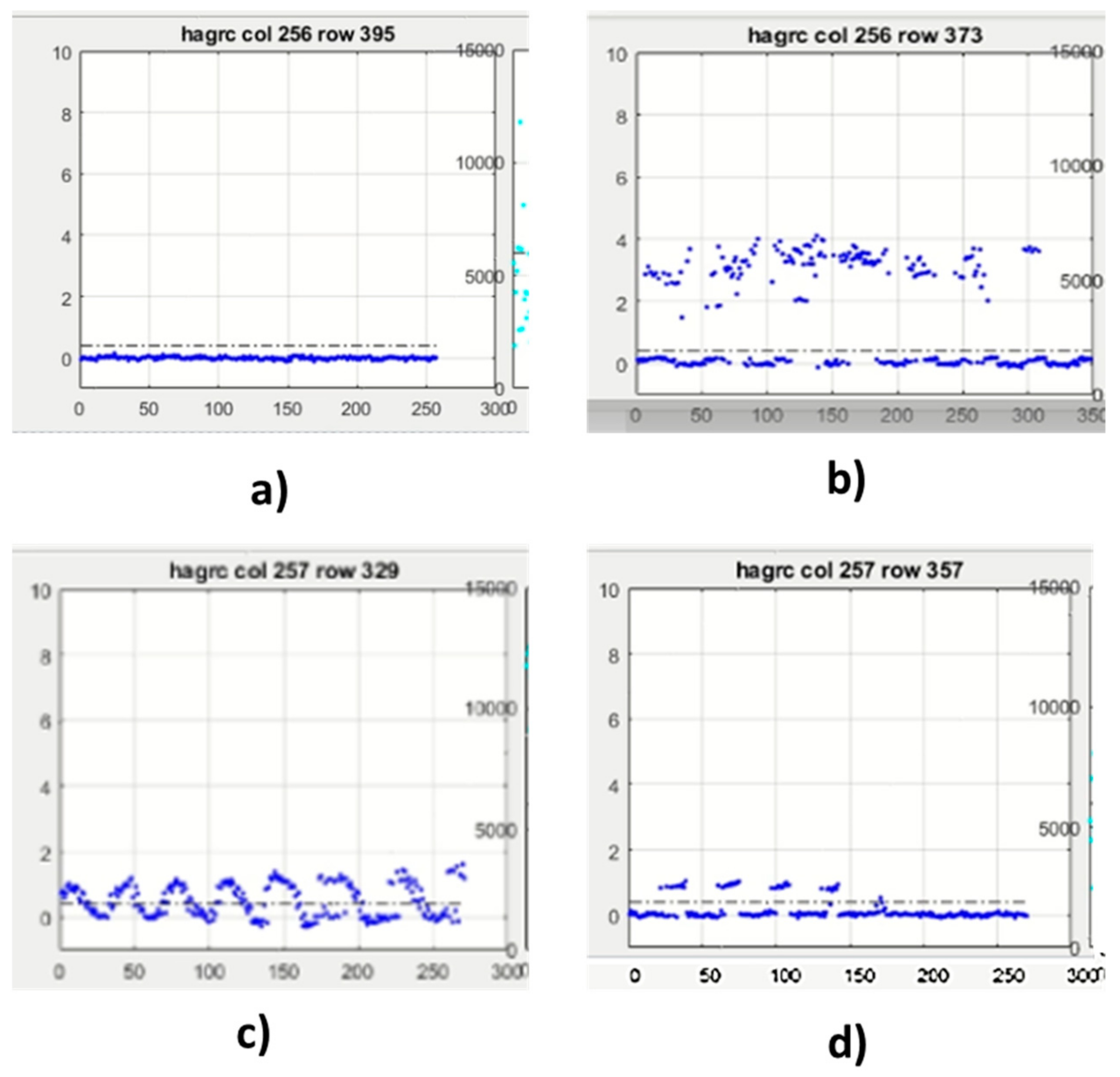
As mentioned earlier, an advantage of the airborne LiDAR over optical cameras is that it includes points on surfaces that are covered by foliage. To extract the segments of roads under foliage, a moving filter consisting of the same block of silos was used to determine whether they were on a road. For this, a small block of neighboring silos was combined to form a larger set. The Mahalanobis distance of the points within this set is used as a criterion first to find points that are aligned to the general direction of the road. Once these points are identified, a second filter consisting of attributes such as HAG, intensity, and reflectance (

Table 3. Typical Threshold Values for Filter 2.

Attribute	Threshold
HAG	0.4 m
Normalized Intensity	0.1068
Reflectance	0.03

) was applied to determine points that were likely to lie on the road. The newly discovered points are added to the existing set of road points. This filter was propagated sequentially along horizontal and vertical stripes to fill out the gaps in roads formed by overhead foliage.

The results of this process are presented here. Here as the road surface was being developed by the algorithm, 3 separate snapshots at the beginning, middle, and end of the process have been shown in Figure 11. In this example, a roughly 8.5 m length of the road hidden under foliage was recovered using this process.

4. Discussion

We have described a simple, fast method of data reduction and extraction of information from massive LiDAR data sets. Since the GM-APD LiDAR data is dense and covers large areas with very high resolutions, it is difficult to validate the statistics of this method such as geo-accuracy, probability of correct and false identifications, etc., on a sufficiently large scale. High-resolution imagery with EOIR sensors is available from airborne and satellite platforms, but these can provide only 2D image data. Their accuracy depends on many factors. For visible sensors, the precision is affected by factors such as the location of the illuminating source such as the sun, the BRDF, and relative contrasts of materials on and in the neighborhood of roads, as well as environmental conditions such as humidity, the wetness of surfaces, etc. For IR cameras, the limitation of 2D imagery also applies along with lower resolution. Satellite-based imagery is mostly intended for use in navigation purposes, which high accuracy and resolutions comparable to GM-APD LiDAR data are not needed nor available. For true validation, large-scale surveys on the ground of the road surfaces imaged by the Airborne LiDAR are needed. On a very small scale, a validation of this measurement method was described in Section 2 above. In this case, FEMA has contracted an independent surveyor to take measurements of the breach on the road which had previously been measured using LiDAR data. The surveyor had used a precision ranging device aboard a drone flying at close range to the ground to take high-accuracy measurements. When the dimensions of the remote-sensed breach measurements with LiDAR were compared with the close-range measurements, the different dimensions were found to be less than 1%. For true validation, a large-scale exercise of measuring samples of dimensions of the road on the ground is needed. This validation effort was outside the scope of this project but may be undertaken in the future.

Future Work

The approach applied in the algorithm to find roads can be extended beyond roads to find other types of structures including buildings, foliage, bridges, towers, power lines, and parking lots with cars. In Figure 12, we show examples of point clouds of roads, trees, landscaped shrubs, and a parking lot with vehicles.

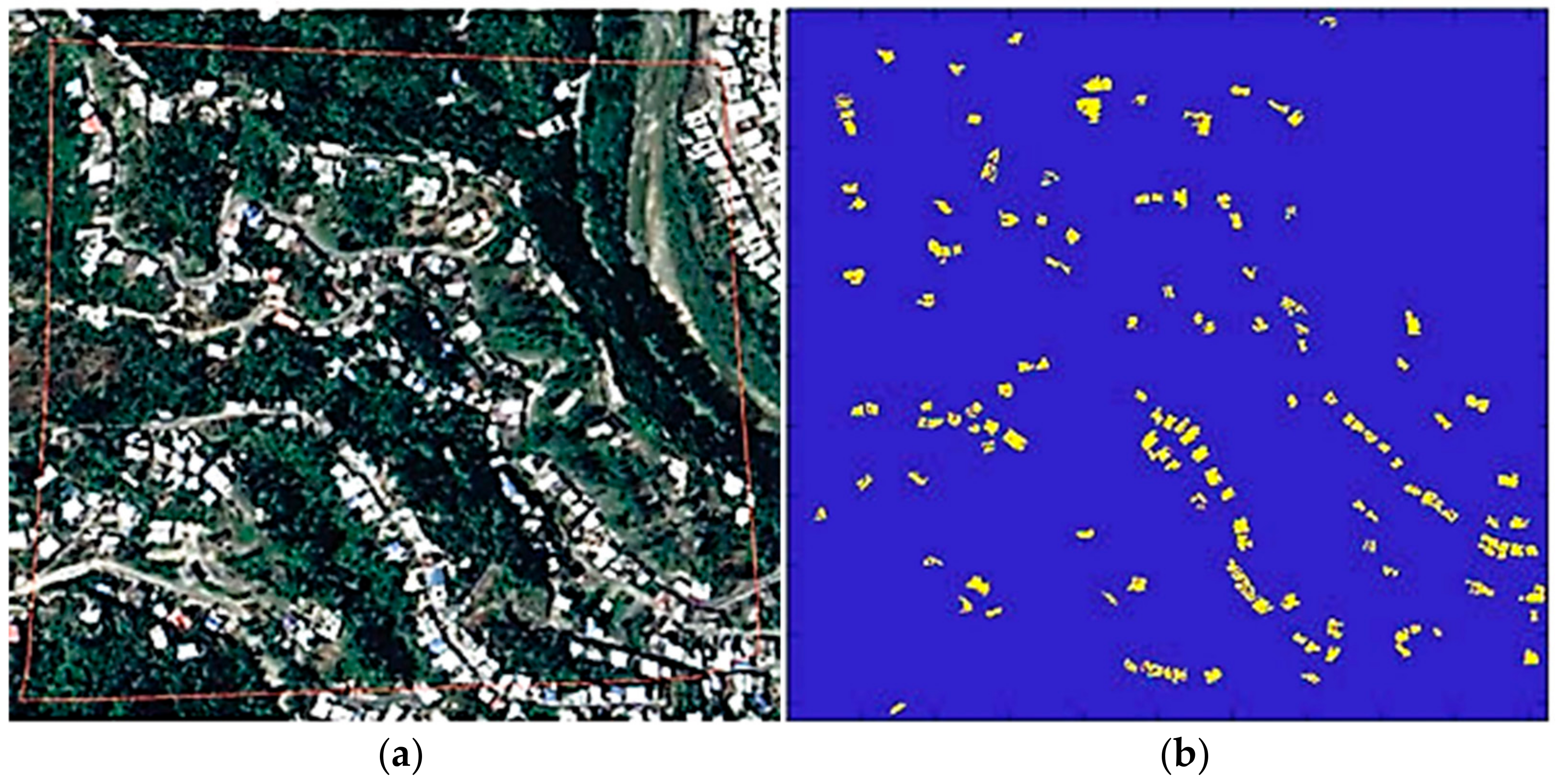
We briefly experimented using the algorithm tuned for roadway assessment to identify buildings (Figure 13). The algorithm was modified to account for those buildings with heights of at least 10 feet and that the point density of points on rooftops will generally be higher with small variations. Figure 13 illustrates the algorithmic output after adjusting the thresholds when processing the HAG positions. Similar to roadways, once the buildings are identified, their dimensions such as height, the gradient of roof slopes, and precise 3D dimensions of damaged sections could be measured.

Future use of this algorithm will be in developing sufficient quantities of data-sets for training neural networks to perform the automated road-finding task. Although the approach described in this paper is effective for a few tiles, the threshold values selected in the filter needed to be adjusted just ever so slightly depending upon the environmental conditions, the materials used for constructing the physical structures, and other factors. In situations where adequate time and computing resources are available, the application of AI with sufficiently large training sets may provide a robust approach for fast, automated recognition of physical structures of interest.

Additionally, the algorithm was designed to only leverage homogenous LiDAR information, yet LiDAR alone is insufficient to meet the public assistance needs. While a LiDAR point cloud will enable FEMA to characterize the erosion of a mountainside road, LiDAR will not identify which road is damaged. Fusing LiDAR with open-source geospatial information is a necessity.

Weather forecasts and data are another important consideration since the AOSTB 1064 nm laser doesn’t penetrate clouds. Note however that not all LiDAR systems are as severely impacted by cloud cover. Atmospheric particulate and moisture are also important. Notably Saharan dust from Africa will influence the atmospheric conditions over the Caribbean but more research is required to determine how it affects LiDAR-derived PED products. Research is required to determine if satellite imagery could be used to identify or explain potentially degraded LiDAR returns. Another supercomputing application would be the production of a metric from previous flights that indicates the probability of poor cloud or dust conditions by area to guide the prioritization of future surveillance targets.

5. Conclusions

The use of LiDAR imagery has fundamentally changed the methods and approaches used by field surveyors and damage assessors. While visiting sites for inspection, the site assessor no longer needs to take detailed measurements of all the physical features required for quantitative estimates. Instead, the site assessor can focus on taking accurate measurements of a few strategically selected features of physical structures at or near the site. Back in the office, these measurements can be used as references for validation of the location, orientation, and relative scaling of features in the LiDAR image data. The availability of richly detailed 3-dimensional information embedded in LiDAR data offers the possibility of improving the efficiency of damage assessment by FEMA and other agencies. At the same time, the high volume and density of data make it challenging to expeditiously extract actionable information that could be used for recovery from natural disasters on a large scale. Leveraging the work done in the past, we have developed a simple, fast silos-based algorithm for finding roads using combinations of signal attributes and geometrical features embedded in LiDAR data for finding roads that are extendable to finding other physical structures. By adapting different parameters of the Silos filter, structures such as communication towers, water towers, etc., can also be identified in the LiDAR data. Statistical measures such as Hellinger, Matusita, or Bhattacharya distances may be used for the classification and extraction of other types of features and physical structures. Once roads and other physical structures are identified, the process of a highly accurate quantitative assessment of site damages may be performed.

Additionally, LiDAR alone PED is insufficient to justify public assistance scoping and cost estimates. Scoping and costing require applicant-specific information, decisions on methods of repair, knowledge of labor costs, material costs, and policy. There is an operational need to concurrently use and fuse other sensing modalities with the GM-APD LiDAR. As an example, since LiDAR measurements contain no color information, other sensing modalities can assist its material classification.