Quality Control Method for the Service Life and Reliability of Concrete Structures

Abstract

In the past few years, there has been an increasing societal and industrial demand for the reliable assessment and design of structural systems with service-life criteria of at least several decades. The life cycle characterisation of engineering structures in terms of an anticipated service life remains a significant aspect of sustainability in the construction industry. This requires special attention to the definition of structural performance under various actions, and to the implemented engineering materials and methods as well as to the inverse identification and monitoring of structural conditions. Subsequently, the focus remains on the development of a holistic performance-based design approach for new and existing structures and infrastructures. This paper presents the fundamental reliability concepts of performance-based design, with a focus on lifetime assessment. Case studies from actual structural components’ design are used to verify the proposed methodology and indicate the significance of quality assurance in the lifetime assessment of engineering structures. We also confirmed that reliability and quality assurance criteria are strongly connected. Therefore, a methodology for quality-based service life assessment is presented and elaborated in the case studies.

1. Introduction

The inclination of the engineering society towards sustainable industries is evident in many facets of modern life and business. Current research focuses on sustainability as a fundamental requirement, based upon a holistic treatment of societal needs and impacts, life-cycle cost and environmental impact. The treatment of the existing building stock competes with the building of new projects in terms of resource volumes, with an increasing trend. This dictates the necessity to introduce codes and standards that coherently address new and existing structures. The safety of users, third parties and the environment; serviceability and durability; and other specific performance criteria, such as robustness and resilience, form the focus of upcoming design standards. Simultaneously, inherent uncertainty of materials and the environment, along with rapid technological advancements and innovations, create an increasing need for decisions based on reliability and holistic design concepts. State-of-the-art performance-based design is required to (a) address the structural safety and reliability of structures by use of analyses with various levels of complexity and accuracy, (b) assess the structure’s condition during service life with inspection, testing and monitoring and (c) define necessary intervention practices. In Figure 1, the Ishikawa causal diagram with the analysis of causes and factors of material degradation is illustrated.

During the implementation of life-cycle-management strategies, these intervention actions must be selected in order to maintain assets at a desired performance level. Therefore, specific performance indicators must be established at a technical component level. These indicators can be qualitative or quantitative, and they can be obtained during principal inspections through visual examination, a non-destructive test or a temporary or permanent monitoring system. The indicators derived compared with target performance indicators allow for the evaluation of adherence to the owner- or user-defined quality requirements. In this framework, quality is understood as fitness for purpose, or the degree to which a set of inherent characteristics of a product or service fulfils its requirements. The quality requirements are observed through a project-specific quality control (QC) plan. The QC plan specifies all activities and tools needed to ensure the quality requirements related to the investigated performance aspects (safety, serviceability, etc.). It can define the type and quantity of data necessary to assess the performance indicators of the structure or its individual components at the time of data collection and in the future. A QC plan should also include decision models for maintenance actions based on the forecast of performance indicators. In this sense, the QC plan overlaps with the strategic asset management plan (SAMP) as defined by the International Organization for Standardization [1].

The current work will help to fill the gap in the research that can be seen in less elaborated aspects of Eurocodes, namely the connection of reliability and execution classes [2,3,4]. In addition, this work reinforces the outcomes of the COST TU 1406 project in terms of standardisation of quality specifications. In other words, the present study aims to confirm an interconnection of life-cycle reliability measures with elements of QC and quality assurance by elaborating on the principles of reliability as applied to structural engineering problems. In addition, typical quality criteria with an emphasis on concrete structures are presented. These are translated to reliability principles through a methodology based on the reliability index β. This theoretical approach is then applied to two realistic case studies, being the durability assessment against concrete carbonation and chloride ingress, based on [5]. In these cases, quality is expressed through the concrete specifications in the selection and QC, mainly for the cement type and the water–cement (w/c) ratio. Two supplementary examples are used as case studies for the effects of quality defects on the load bearing reliability of structural components. The first one discusses the reinforcement placement tolerances in a one-way slab. The second example discusses the installation quality of bonded anchors in concrete. These examples are considered by the authors as suitable for demonstration and relevant to practice, without excluding the fact that the basic principles and tools apply to other types of materials, limit state functions and damage processes. The results of these demonstrative analyses are discussed in the final section of the paper, where the main conclusions of the study are highlighted, and practical recommendations are provided in relation to the sensitivity of a structure’s reliability in terms of quality issues and the significance of the construction phase on the whole-life performance of a structure.

2. Reliability Concepts

Educated decisions for engineers fundamentally depend on the designed or constructed system’s failure probability. Reliability is then understood as the probability that an item or facility will perform its intended function and, as such, as the complement of the probability of failure p_f. In its most basic formulation, reliability r is described by Equation (1):

$$r=1-p_f.$$

(1)

In general, the design requirement is expressed in the form of a limit state function (LSF), where, e.g., resistance is greater than the load effect, as expressed by Equation (2):

$$G=g\left(X\right)=R-S,$$

(2)

where x is the set of random variables (time dependent or independent), G = g(X) is the limit state function (with g(X) < 0 being the failure state), R is the resistance and S is the load action.

The general solution for the estimation of the failure probability (p_f) can thus be obtained through the integral between –∞ and +∞, as shown in Equation (3).

$$p_f={{\displaystyle \int }}_{-\infty }^{+\infty }{f}_S\left(X\right)·F_R\left(X\right)\mathrm{dx},$$

(3)

where f_S is the probability density function (PDF) of the limit state function S and F_R is the cumulative distribution function (CDF) of the limit state function R.

To quantify the reliability of the system based on the LSF, the Cornell reliability index β can be estimated based on the individual probability functions of the LSF input, G = R − S [6]. Although the reliability assessment concept is universal, the specific mathematical formulation presented herein requires that R and S follow normal distributions and are statistically independent. The reliability index is defined as

$$\beta =\frac{{\mu }_R-{\mu }_s}{\sqrt{{\sigma }_R^2+{\sigma }_s^2}},$$

(4)

where μ_R and μ_S are the mean values of resistance and load action, respectively, and σ_R and σ_S are the standard deviations for resistance and load side, respectively.

Then, the failure probability p_f can be estimated as:

$$p_f=\varphi \left(-\beta \right),$$

(5)

where $\varphi$ is the standard normal probability function.

The main characteristics and limitations of the Cornell reliability index concept are that it is limited in the number of variables, it can be applied only to linear limit state functions, it considers only normally distribute variable and there should be no correlation between variables (see [7,8]).

Reliability is typically understood as the property of a system’s reliability (multiple-failure modes) but also that of a component’s reliability (single-failure mode) at a specific point in time. However, rational concepts need to accommodate life-cycle effects, such as the natural deterioration of materials, extreme events and alterations in human activities and environmental conditions, in long-term considerations [9]. These aspects are particularly governed by uncertainties, where probability-based concepts also find a more efficient implementation. In such cases, the reliability verification of a structure should be related to the structure’s service life and failure is associated with two types of events, (a) first peak value beyond an action threshold and (b) the accumulation of propagating damage beyond a resistance threshold. These can be described with time-variant input variables. Consequently, the accepted (target) reliability threshold is also dependent on the lifetime interval under consideration. The service life requirement can be associated with the target reliability based on Equation (6), and assuming that the failure events per year are statistically independent, the values of β for different reference periods can be calculated.

$$\Phi \left({\beta }_n\right)={\left[\Phi \left({\beta }_1\right)\right]}^n,$$

(6)

where β_n is the reliability index with respect to n time intervals (years), β₁ is the reliability index with respect to 1 year and n is the reference period (service life) in years.

Target-failure probabilities and associated reliability indices for different types of structures are normally defined in national or international standards, such as Eurocode 0 of the European Committee for Standardization [10,11]. For ultimate limit states, values in the range of p_f = 10⁻⁵ to 10⁻⁷ and β = 4.0 to 5.0 per year are used, while in serviceability limit states, the failure probabilities (and, accordingly, the reliability indices) are decreased by 1 or 2 orders of magnitude. These values also depend on the structure’s consequence class (CC) attributed to the design. These three consequence classes can then be associated with three reliability classes (RC) (see

Table 1. Definition of consequence classes as per [10] and associated target reliabilities and failure probabilities for different reference periods.

CC/RC	Description of Consequence Class (CC)	Reliability (β) and Associated Probability of Failure pf
		1 Year	50 Years
1 (High)	High consequence for loss of human life. Enormous economic, social or environmental consequences, e.g., grandstands and public buildings.	β = 5.2, pf = approx. 10−7	β = 4.3, pf = approx. 10−5
2 (Medium)	Medium consequence for loss of human life. Considerable economic, social or environmental consequences, e.g., residential and office buildings.	β = 4.7, pf = approx. 10−6	β = 3.8, pf = approx. 10−4
3 (Low)	Low consequence for loss of human life. Small or negligible economic, social or environmental consequences, e.g., agricultural, storage buildings or greenhouses.	β = 4.2, pf = approx. 10−5	β = 3.3, pf = approx. 10−3

for the paradigm of Eurocode 0). Furthermore, they are adopted accordingly for reference periods corresponding to the structure’s design service life. These target values are originally specified according to experience based on engineering judgement and on calibrations against previous practice. In principle, however, target reliabilities can be designated based on customised criteria, such as cost optimisation, risk-acceptance criteria for the safety of individuals and groups affected by the failure of the structure or the life quality index (LQI) approach. Exemplarily, adjusted reliability levels are proposed to assess existing structures or temporary works.

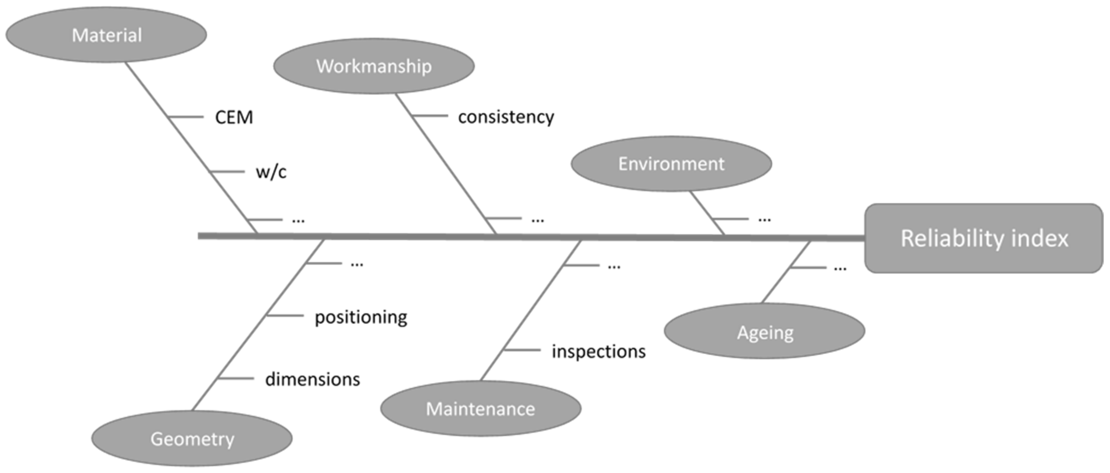
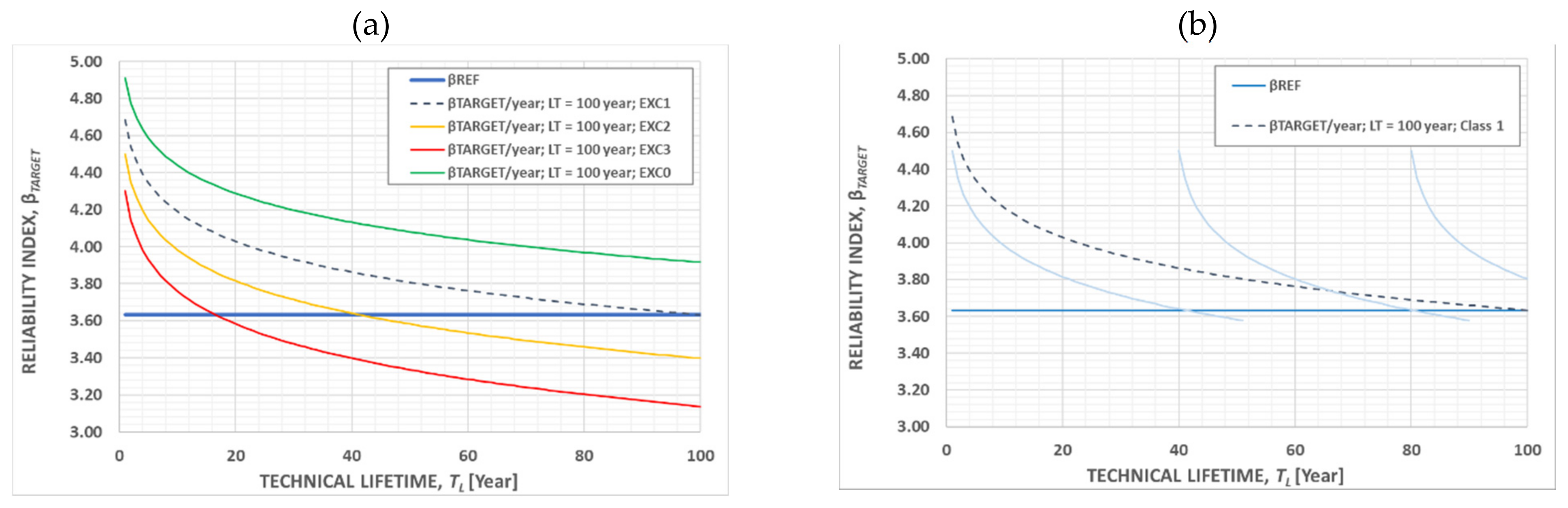
3. Characterisation of the β Index vs. QC

A time-dependent reliability index can be efficiently used to define the quality criteria of a structure as per design and depending on the execution quality. Assuming an asset with a design service life of 100 years (typically required for transport infrastructure) and a “medium” reliability class (RC2) as per Table 1, the reliability level at the end of the reference period of t_L = 100 years is expected to decline from β₀ = 4.7 (p_f = 10⁻⁶) per annum to β₁₀₀ = 3.63 (p_f = 1.4·10⁻⁴). This value is also assumed as the target value for the reference period, below which the structure does not serve the set requirements. This can then also be used as the reference value for determining the economic gain or loss of an investment related to the quality of execution.

Depending on the standards adhered to, a classification is recommended for the design supervision, construction inspection, materials and tolerances, as in Annex B of [10], or for concrete and steel structures, as in [11,12], respectively. In addition, there are individual authorities or sector standards, such as the one mentioned in [13], which are valid in Austria. When a component is assigned a reliability class (RC2 in the demonstrated case), in principle, the project-execution class is also adjusted at the same (medium) level. However, this can be varied as per the owner’s intent or the structure’s particularities. This is also reflected in Figure 2, assuming a variation in the construction execution quality while maintaining a uniform design standard. Figure 2 presents the reliability index curves over the technical lifetime of a structure based on a classification according to [13]. This overall execution classification (EXC) includes four rating classes, from 0 to 3, that correspond to a decreasing execution quality in the original construction (where 0 = best and 3 = worst).

Based on the presented assessment, reduced uncertainty in action and resistance models and the execution of good standard can lead to a higher reliability, with a reliability index increase of 0.3 at β_0,EXC0 = 5.0/year and, consequently, a theoretical service life t_L,EXC0 > 100 years. This can be translated to a significant economic profit for the asset stakeholders due to a higher-quality and thus higher-reliance asset throughout its service life, associated with a prolonged operational timeframe.

On the contrary, a substandard or bad execution quality leads to lower initial reliability indices and correspondingly reduced service lives. As noted above, the theoretical formulations (Equation (6)) applied and presented in Figure 2a show a decrease in the target reliability from β₀ = 4.7 /year to β₁₀₀ = 3.63 in 100 years for RC2 (dashed line). Assuming the mathematical formulation of Equation (6), this target reliability can be used as a reference for the investigated case. For a substandard execution quality (assumed here as Class 2 according to RVS standards (RVS stands for Richtlinien und Vorschriften für das Straßenwesen)) [14], a reduced initial reliability index of β_0,EXC2 = 4.5 can be assumed. In this case, (the amber line in Figure 2a), the reference target reliability of β = 3.63 is already reached at just over 40 years of operation. This indicates a loss of 60 years in the technical lifetime of the asset, already identified immediately after completion of the construction. For a bad-quality construction, a greater reduction in the annual target reliability can be observed, for instance, β_0,EXC3 = 4.3.

Note that the assessment herein does not account for the degradation process in the structural materials or for improvement interventions, such as repair and strengthening measures. Furthermore, it disregards the assessment of the asset’s conditions through inspections, monitoring or non-destructive and destructive testing. If an assessment procedure is implemented, there is a possibility to extend the expected service life of the asset due to a reduction in the uncertainty regimes. This is graphically represented in Figure 2b. Here, the same situation detailed above is discussed, assuming a bad execution quality, i.e., Class 3 according to the RVS standards. The difference in this case is that a testing or interval-monitoring procedure is implemented in order to guarantee the condition and, thus, the reliability of the structure. As illustrated, this assessment process and accordingly the definition of the reliability level β can be processed each time when the reference line of β₁₀₀ = 3.63 is violated, for example, at 40 and 80 years. This periodical assessment of the reliability level β associated with the respective technical assessment procedures can be understood as a periodic updating strategy according to the upcoming Model Code 2020.

4. Case Studies on Durability

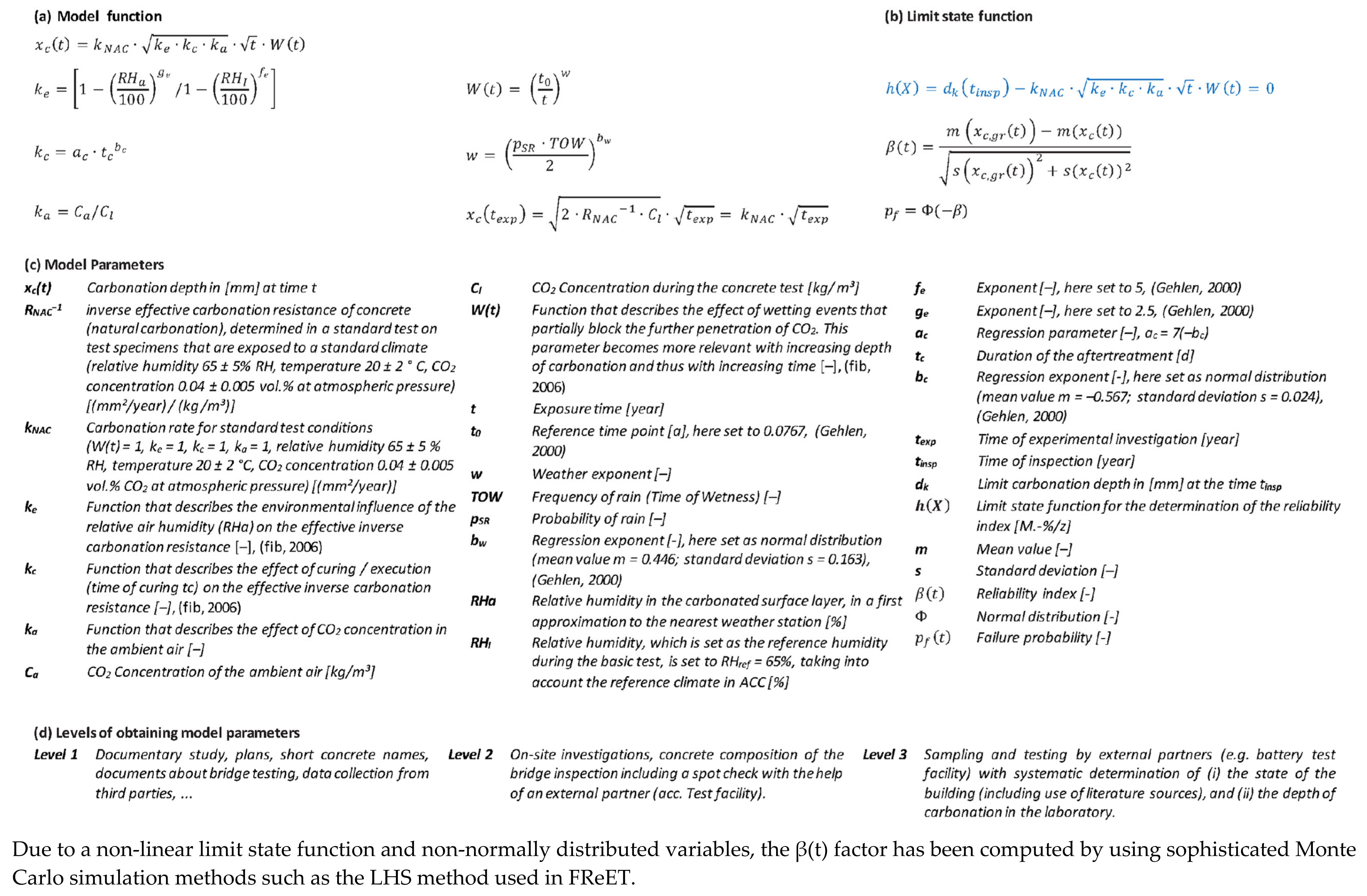
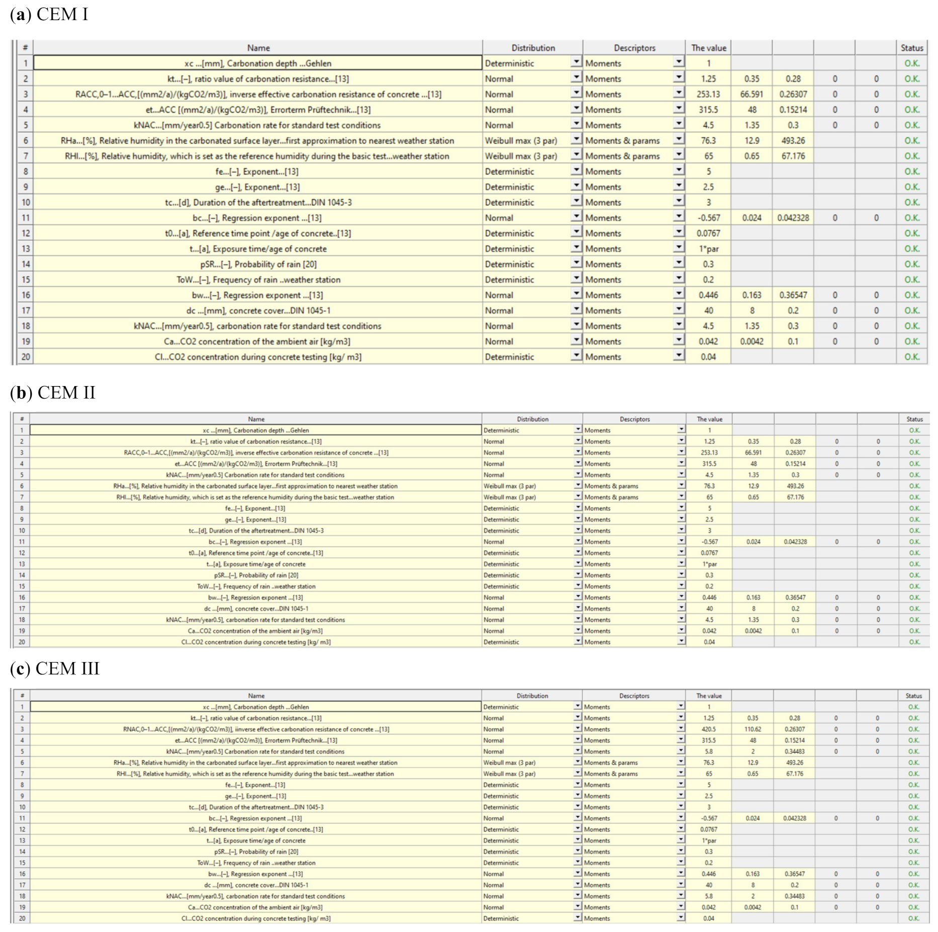
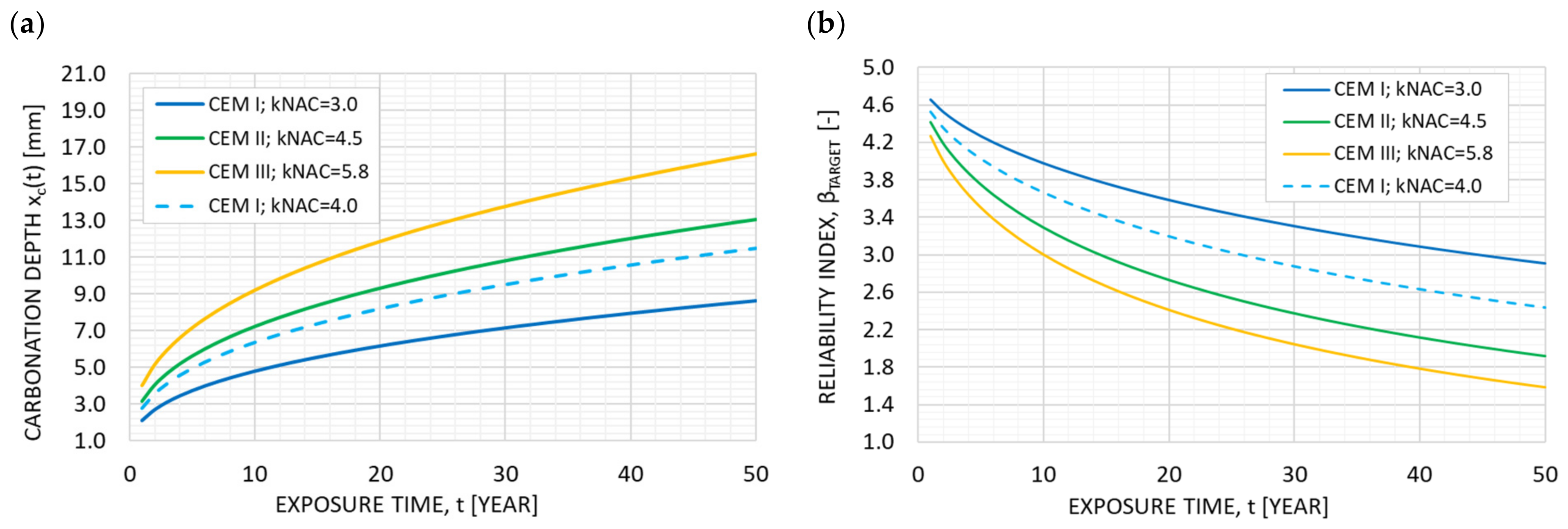
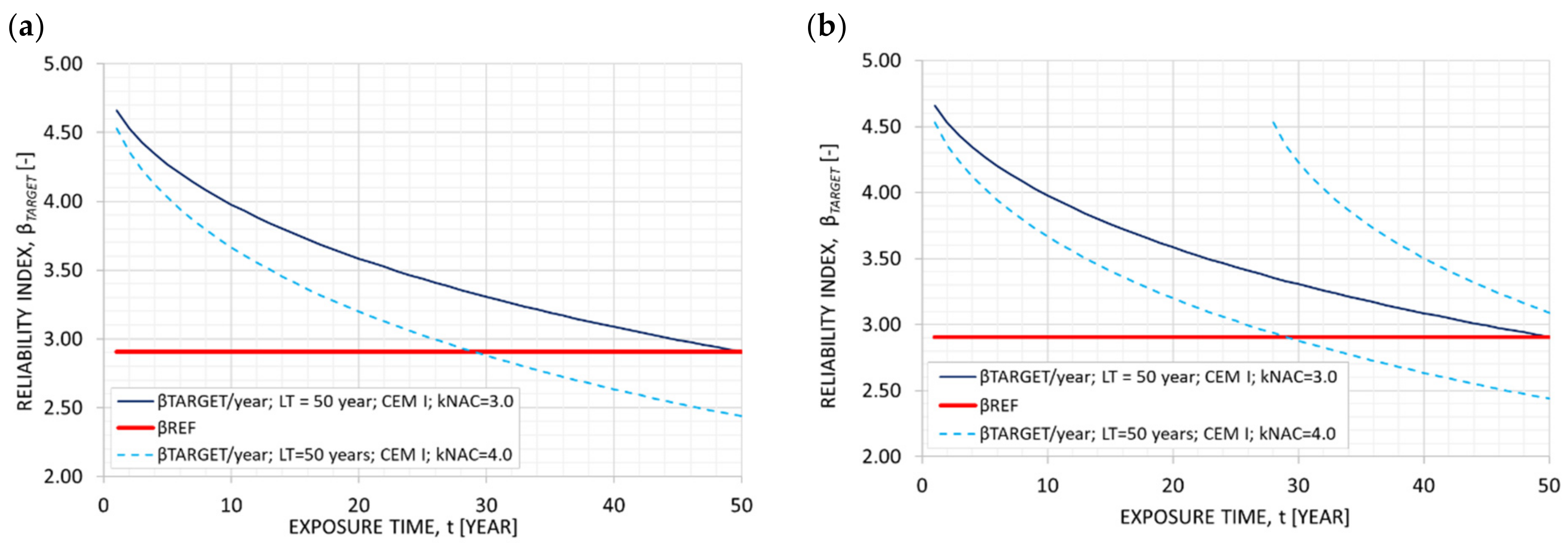
As a state of practice, durability is specified through empirically limiting values (max. w/c, min. binder content, minimum reinforcement cover) defining the resistance of concrete elements against actions of the service environment, while environmental action is characterised by exposure classes. Models for describing the environmental actions are used to carry out a lifespan assessment, and the element’s resistance against these actions needs to be accounted for as well. Both the actions and the mechanisms of damage are extremely complex, and their exact physical or chemical modelling cannot be described without a realistic elaboration of several significant parameters and associated uncertainties. A vital part of such modelling addresses the carbonation and chloride penetration in the concrete, which are presented below in detail. In the presented cases, particular focus is drawn to the used w/c ratio during concrete production and its consequences for the durability-related material parameters. Moreover, the effect of the selected cement types (CEM I, II or III) on the specification and construction of the structure is a driving parameter with a significant impact on the structure’s durability-related reliability assessment.

4.1. Carbonation

In performance-based durability design with regard to carbonation, the carbonation process is described through the carbonation-prediction model presented in

Table 2. Model parameters of the carbonation model.

Variable	Symbol	Unit	Default Value	Level for Obtaining the Model Parameters	Test Procedure, Test Details	Literature and Background Information	Distribution *	Maximal Value	Minimal Value	Mean Value	Standard Deviation
①	②	③	④	⑤	⑥	⑦	⑧	⑨	⑩	⑪	⑫
(1a) RNAC−1		(mm2/year)/(kg/m3)	-	3(ii)	[17,18,19]	[5,9,20,21,22,23,24,25,26]	N			μ	Σ
(1b) kNAC (alternative)		mm/year0.5	-	3(i) and 3(ii)	[5,20]	[5,9,20,21,22,23,24,25,26]	N	11	1	μ	σ
(2) kc	bc	—	-0.6	3(i)	-	[5,9,20,21,22,23,24,25,26]	N	−0.5	−0.8	–0.6	0.25
	tc	days	3	1 and 3(i)	-	[5,9,17,20,21,22,23,24,25,26]	K	7	2	μ	—
(3) ke	RHa	%RH	75	1, 2 and 3(i)	-	[5,9,21,22,23,24,25,26]	W	85	75	μ	σ
	RHl	%RH	65	1, 2 and 3(i)	-	[5,9,21,22,23,24,25,26]	K	65	65	65	—
	ge	—	2.5	3(i)	-	[5,9,17,20,21,22,23,24,25,26]	K	2.5	2.5	2.5	—
	fe	—	5	3(i)	-	[9,21,22,23,24,25,26,27,28,29]	K	5	5	5	—
(4) W(t)	ToW	—	0.2	1 and 3(i)	-	[5,9,20,23,24,25,26]	K	0.5	0	μ	—
	pdr	—	0.3	1 and 3(i)	-	[5,9,20,23,24,25,26]	K	0.6	0	μ	—
	bw	—	0.3	1 and 3(i)	-	[5,9,20,23,24,25,26]	K	0.71	0.24	0.5	0.16
	t0	year	0.767	1	-	[5,9,20,23,24,25,26]	K	0.0767	0.0767	0.0767	—
(5a) Ca		kg/m3		3	-	[5,9,20,23,24,25,26]	N			μ	σ
(5b) ka (alternative)	Ca	vol.%	0.042	1 and 2	-	[9,25,26,27]	N	0.044	0.036	μ	σ
	Cl	vol.%	0.044	3b	-	[25,26,27]	K	0.044	0.044	0.04	—
(6) c		mm	35	1, 2 and 3	-	[25,26,27]	N	85	15	μ	σ
(7) tSL		year	100	1 and 3	-	-	K	120	1	50	—

* Normal distribution, N; lognormal distribution, LN; beta distribution, B; constant, K.

. Specifically, Figure 3a shows the basic function of the carbonation formulation, along with the complementary functions of the fib Model Code for Service Life [9]. This basic function is transformed to a limit state function for the definition of the β index (Figure 3b) according to the classical Basler–Cornell approach and, therefore, can be further used to define the failure probability p_f. The necessary input variables, indices and parameters for the function of Figure 3a are listed in Figure 3c, along with the symbols used in the fib Model Code 2010 presented in [15,16], the units and some suggested values proposed in the literature. The models presented in Figure 3a,b and their input parameters can be obtained through various inspection levels, as shown in Figure 3d.

There is a difference in the forms of survey between classical inspection (Level 1), the more detailed on-site inspection (Level 2) and laboratory testing (Level 3). A more detailed classification of the inspection levels to obtain the model parameters is presented in Table 2.

Table 2 provides global information that is useful for stakeholders involved in this assessment procedure. In particular, it provides a general overview of the common default values to be used in the model function (column ④), the level of inspection for each parameter with reference to Figure 3d (column ⑤), the testing methods to obtain each model parameter (column ⑥) and the respective literature source in which the parameters are described (column ⑦). Table 2 also presents statistical descriptions of certain values (grey-shaded areas, columns ⑧ to ⑫), such as the distribution type, the minimum and maximum values, the mean value and the standard deviation for each parameter.

As mentioned above, the equations in Figure 3b are used to calculate the reliability index β of the model function.

Table 3. Reliability index β vs. failure probability p_f.

Reliability index β	0	1	2	3	4	4.5	5
Failure probability pf	50%	15%	2.3%	0.1%	0.03%	0.003%	0.0005%

presents the relationship of the reliability index β with the failure probability for clarity and further reference in the paper. Specifically, the value of k_NAC of the model function that corresponds to certain carbonation-resistance classes depends on the type of cement and the w/c ratio, as indicated in

Table 4. W/b ratios depending on the cement type and the carbonation resistance class according to [25,26].

Resistance Class		2	3	4	5	6	7
Ranges of kNAC (mm/year0.5)		1 < kNAC ≦ 2	2 < kNAC ≦ 3	3 < kNAC ≦ 4	4 < kNAC ≦ 5	5 < kNAC ≦ 6	6 < kNAC ≦ 7
Cement type	CEM I	0.45	0.50	0.55	0.60	0.65	–
	CEM II/A	0.45	0.50	0.55	0.60	0.65	–
	CEM II/B	0.40	0.45	0.50	0.55	0.60	0.65
	CEM III/A	0.40	0.45	0.50	0.55	0.60	0.65
	CEM III/B	–	0.40	0.45	0.50	0.55	0.60

, for a range of typical boundary conditions relevant to practice.

Table 5. Proposals for unfavorable climatic conditions according to [25,26].

Exposure Class		RHa (%)	ToW (–)	pdr (–)
XC1	Dry	≥65	=0.0	=0.0
XC2	Wet	≥90	=0.0	=0.0
XC3	Outdoor, sheltered	≥75	=0.0	=0.0
XC4	Outdoor, unsheltered	≥75	≥0.2	≥0.1

demonstrates the classification of the environmental or exposure classes (XC1 to XC4) and the respective values for each exposure class that correspond to unfavourable environmental conditions. Similarly,

Table 6. CO₂ concentration Ca in ambient air according to [25,26].

Exposure Class			CO2 Concentration Ca (vol.%)
			Mean Value μ	Standard Deviation σ
XC1	Normal	Indoor	0.036 ≦ μ ≦ 0.043	0.0010 ≦ σ ≦ 0.0080
XC2	Normal	E.g., foundation	0.036 ≦ μ ≦ 0.043	0.0010 ≦ σ ≦ 0.0080
XC3/XC4	Normal	Rural	0.036 ≦ μ ≦ 0.042	0.0010 ≦ σ ≦ 0.0055
		Urban	0.038 ≦ μ ≦ 0.043	0.0015 ≦ σ ≦ 0.0080

presents the mean value and the standard deviation of CO₂ concentration Ca in ambient air for each of the aforementioned exposure classes. Thus, Table 4, Table 5 and Table 6 provide a detailed set of values based on the environmental and cement conditions for the selection of the most appropriate input for the carbonation function of Figure 3a,b.

Keeping in mind the global values presented in Table 2 and using the already presented model functions, a first set of analyses was performed, using the commercial software FReET [30] to calculate the reliability indices β and the carbonation depth. The method used in software FReET to obtain the reliability indices is the LHS-based Monte Carlo simulation; for details, see [31]. The analysis input parameters for each cement type from the software are represented in Figure 4. The analyses were performed for the different cement classes CEM I, CEM II/B and CEM III/B, with a corresponding w/c ratio of 0.55, set into the exposure class XC4. The increase in the carbonation depth in relation to the exposure time for 50 years is as shown in Figure 5a. The CEM I compound shows the best performance (the lowest carbonation depth), with the carbonation front reaching a maximum depth of 8.6 mm after 50 years (solid blue line). The CEM II/B composition shows the same carbonation depth after just 17 years of exposure (solid green line) and for the CEM III/B composition, a carbonation depth of 8.6 mm is reached after less than 10 years (solid orange line) and almost double the one of CEM I at the 50-year service life.

The respective results in terms of the reliability index β are obtained through the limit state function, and they are shown in Figure 5b. For CEM I, the reliability index curve shows a value of β = 2.9 for 50 years. For CEM II/B, it shows a value of β = 1.9 for 50 years, and for CEM III/B, it shows a value of β = 1.59 for 50 years. The initial reliability indices (at year 1) are 4.66, 4.41 and 4.27, respectively. As seen in Table 3, the w/c ratio highly influences the k_NAC values, which in turn strongly control the reliability prediction. Assuming that the cement type CEM I is chosen, with a w/c ratio value of 0.6, the k_NAC value also increases to 4.0. The results of using this input are presented by the dashed blue line in Figure 5, with the mean value of carbonation depth at 50 years’ exposure time increasing to 11.5 mm and the reliability index decreasing to β = 2.44.

In Figure 6a, the reliability index of the exposure time of 50 years for CEM I and the two alternative k_NAC values of 3.0 and 4.0 are presented. It can be demonstrated that, for k_NAC = 3.0 (w/c = 0.55), the β_REF is reached after a technical lifetime of 50 years. In the case of k_NAC = 4.0 (w/c = 0.60), the performance of the structure declines, with the β_REF reached only after 27 years of exposure. Similar to the concept presented in Figure 2b, Figure 6b accounts for an assessment of the asset’s conditions through inspections, monitoring or non-destructive and destructive testing. Through this process, the expected service life of the asset can be extended. As illustrated in Figure 6b, this periodic adjustment, in line with the upcoming Model Code 2020, is applied every time the reliability level β exceeds the reference line of β₅₀ = 2.91, for example, at 27 years.

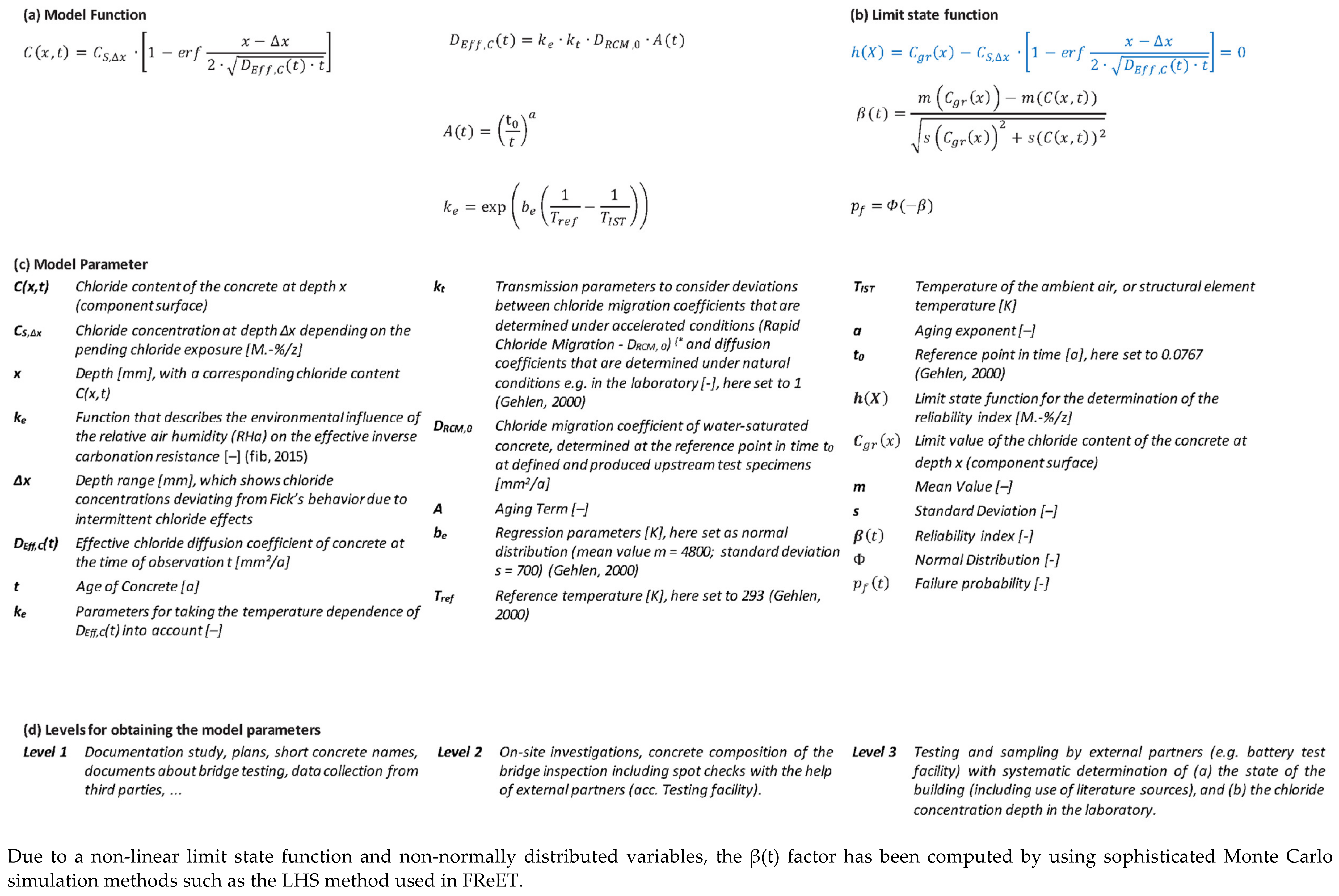
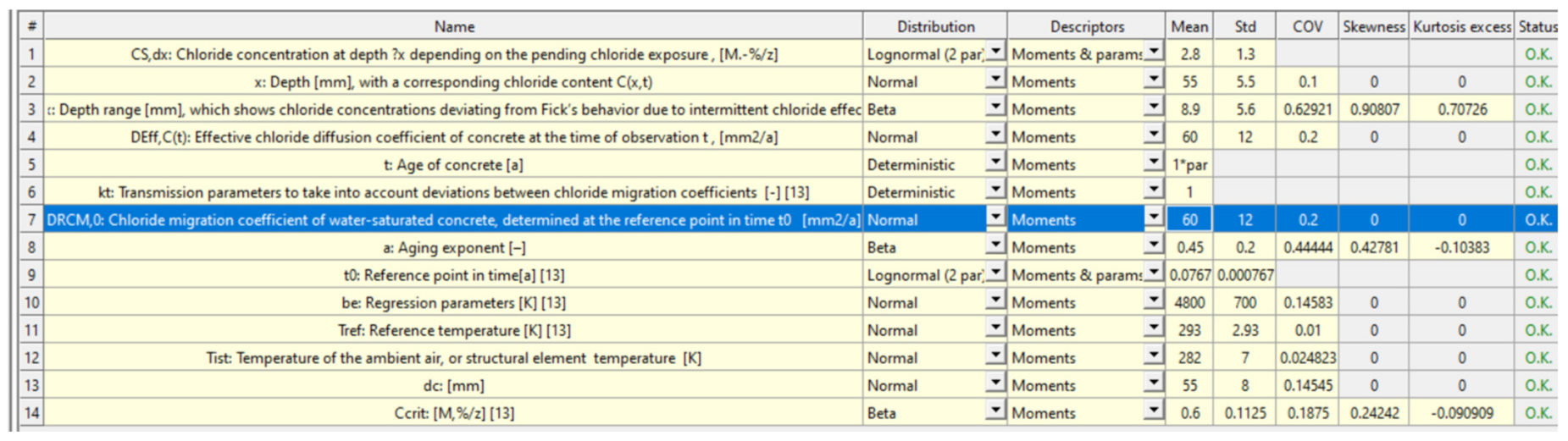
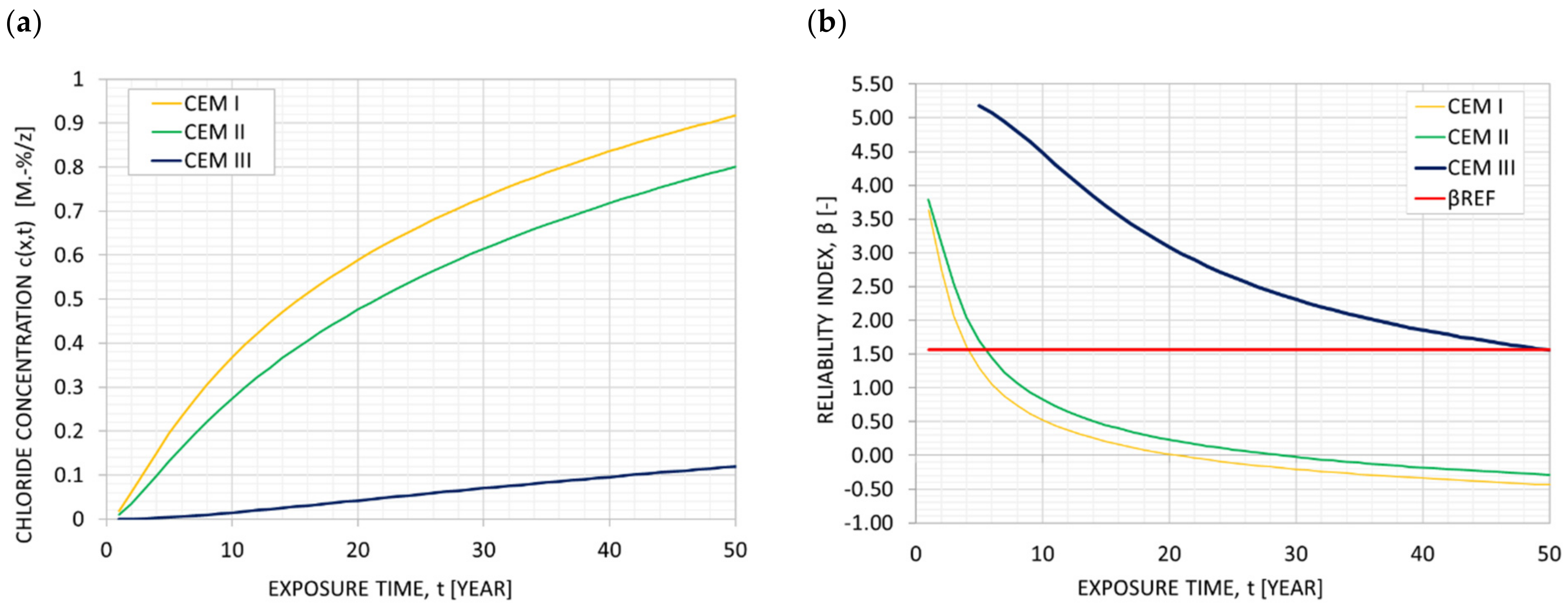
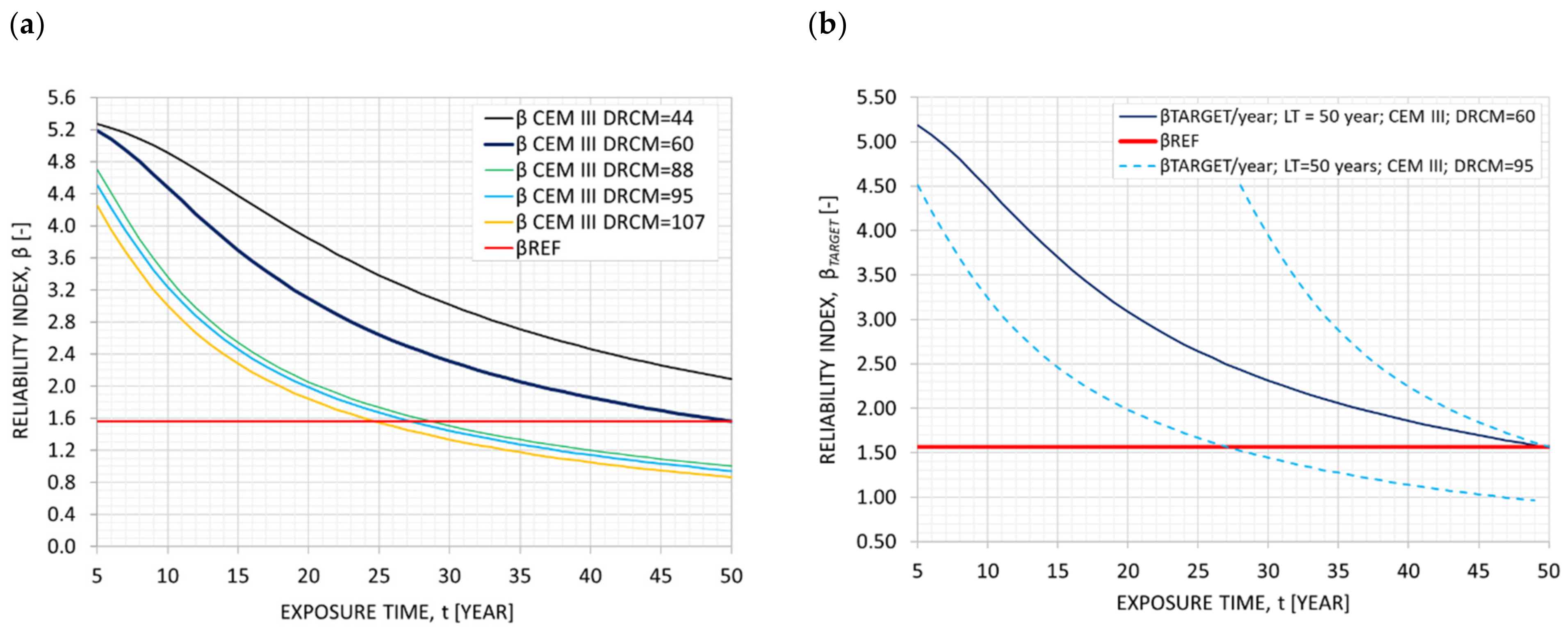
4.2. Chloride Ingress

There are several numerical models to describe chloride penetration in concrete, most of which are based on Fick’s second law of diffusion. In the current study, the modified DuraCRETE model [32] was applied for the time-dependent penetration of chloride in concrete. Specifically, Figure 7a shows the basic function of the chloride ingress formulation, which is also used in the fib Model Code for Service Life Design [9]. This basic function is transformed into a limit-state function for the definition of the β index (Figure 7b), according to the classical Basler–Cornell approach; therefore, it can be further used to define the failure probability p_f, as per Table 3. The necessary input variables, indices and parameters for the function of Figure 7a are listed in Figure 7c, together with their descriptions and suggested values as proposed in the literature. The input parameters of the models presented in Figure 7a,b can be derived through the same inspection levels as with carbonation, repeated in Figure 7d for completeness. A more detailed representation of the inspection levels to obtain the model parameters is presented in

Table 7. Model parameters of the chloride ingress model.

Variable	Symbol	Unit	Default Value	Level for Obtaining the Model	Test Procedure, Test Details	Literature and Background Information	Distribution *	Maximum Value	Minimum Value	Mean Value	Standard Deviation
①	②	③	④	⑤	⑥	⑦	⑧	⑨	⑩	⑪	⑫
(1) C(x,t)		M.-%/z	-	3(ii)		[9,27,28,29,30,31,32,33,34,35,36,37,38,39]	—	—	—	—	—
(2) CS,Δx		M.-%/z	-	3(ii)	[9,27,28,29,30,31,32,33,34,35,36,37,38]	[9,27,28,29,30,31,32,33,34,35,36,37,38,39]	LN	3	0.75	2.6	1.2
(3) x		mm	35	1 and 2		[9,27,28,29,30,31,32,33,34,35,36,37,38,39]	N	80	15	55	5
(4) Δx		mm	5	3(ii)		[9,27,28,29,30,31,32,33,34,35,36,37,38,39]	B	50	0	8.9	5.6
(5) DEff,C(t) (mm2/a)	ke	—	-	3(i) and 3(ii)	[33,39,40]	[9,27,28,29,30,31,32,33,34,35,36,37,38,39]	—	—	—	—	—
	kt	—	1	3(i) and 3(ii)		[9,27,28,29,30,31,32,33,34,35,36,37,38,39]	K	1	2.5	2.5	—
	DRCM,0 CEM I	mm2/a	60	3(i) and 3(ii)		[9,27,28,29,30,31,32,33,34,35,36,37,38,39,40]	N	280	789	320	64
	DRCM,0 CEM III/B	mm2/a	320	3(i) and 3(ii)		[9,27,28,29,30,31,32,33,34,35,36,37,38,39]	N	107	44	60	12
	A	—	-	3(i) and 3(ii)		[9,27,28,29,30,31,32,33,34,35,36,37,38,39]	—	—	—	—	—
(6) ke (-)	be	K	4800	3a	-	[9,27,28,29,30,31,32,33,34,35,36,37,38,39]	N	5950	3650	4800	700
	Tref	K	293	3(ii)	-	[9,27,28,29,30,31,32,33,34,35,36,37,38,39]	K	293		—	—
	TIST	K	280	1 and 2	-	[5,9,27,28,29,30,31,32,33,34,35,36,37,38,39]	N	293	271	282	7
(7) A(t) (-)	aCEM I	—	0.3	3(ii)	-	[9,27,28,29,30,31,32,33,34,35,36,37,38,39]	B	1	0.1	0.3	0.12
	aCEM III/B	—	0.45	3(ii)	-	[9,27,28,29,30,31,32,33,34,35,36,37,38,39]	B	1	0.1	0.45	0.20
	t0	a	0.076	3(i)	-	[9,27,28,29,30,31,32,33,34,35,36,37,38,39]	LN	0.088	0.065	0.0767	0.007

* Normal distribution, N; lognormal distribution, LN; beta distribution, B; constant, K.

.

In a similar way to Table 2, Table 7 also provides a general overview of the common default values used in the chloride ingress model function and the following analysis (column ④). Furthermore, the level of inspection for each parameter (column ⑤), the testing methods to obtain each model parameter (column ⑥) and the respective literature source in which the parameters are described (column ⑦) are presented. Furthermore, Table 7 provides the statistical descriptions of certain values (grey-highlighted areas, columns ⑧ to ⑫), such as the distribution type, the minimum and maximum values and each parameter’s first two statistical moments as used in the chloride ingress analysis herein.

The input parameters of the study below were chosen by assuming an exposure class XD3/XS3, with a minimum concrete cover of c_min = 40 mm and a value w/c = 0.45, according to [27]. The parameters used with the suggestive values for CEM III are shown in Figure 8 as an example of the software input. A durability calculation of the chloride penetration was carried out over a period of 50 years, and the critical chloride concentration was selected as equal to C_gr = 0.60 M.-%/z. Figure 9a shows the chloride concentration at the depth of the concrete cover in relation to the exposure time. The values of CEM III show an improved behaviour compared to CEM I and CEM II. Specifically, after an exposure time of 50 years, the chloride concentration values for CEM III are approximately 9 times lower than those for CEM I. A major factor that influences the durability calculations of concrete for chloride penetration is the chloride migration coefficient of water-saturated concrete D_RCM,0, which is further influenced by the w/c ratio. The results of the reliability index in relation to the exposure time are presented in Figure 9a. It can be seen that CEM III again shows the best performance and has a reliability index β = 1.56 after 50 years, with CEM I and CEM II reaching this reference value after 4 and 6 years of exposure time, respectively.

In a further analysis of durability, the influence of the w/c factor of CEM III on the D_RCM,0 was investigated. The variations in w/c values as an agent of D_RCM,0 were chosen according to Gehlen (2000), and they are presented in

Table 8. Chloride mitigation coefficient D_RCM,0 for CEM III/B used in the analyses displayed in Figure 10.

w/c (-)	DRCM,0 (10−12 m2/s)	DRCM,0 (mm2/year)
0.40	1.4	44
0.45	1.9	60
0.50	2.8	88
0.55	3.0	95
0.60	3.4	107

; the analysis results are shown in Figure 10a. It can be observed that increasing the chloride mitigation factor from 60 to 95 mm²/year reduces the reliability index after 50 years from β_REF = 1.56 to β = 0.94, with β_REF reached by 28 years of exposure time. As per the concept presented in Figure 2b, Figure 10b accounts for a periodic adjustment of the asset’s conditions through inspections, monitoring or non-destructive and destructive testing, which facilitates the extension of the structure’s expected service life. As illustrated in Figure 10b, this assessment process is applied every time the reliability level β exceeds the reference line of β₅₀ = 1.56, for example, at 28 years.

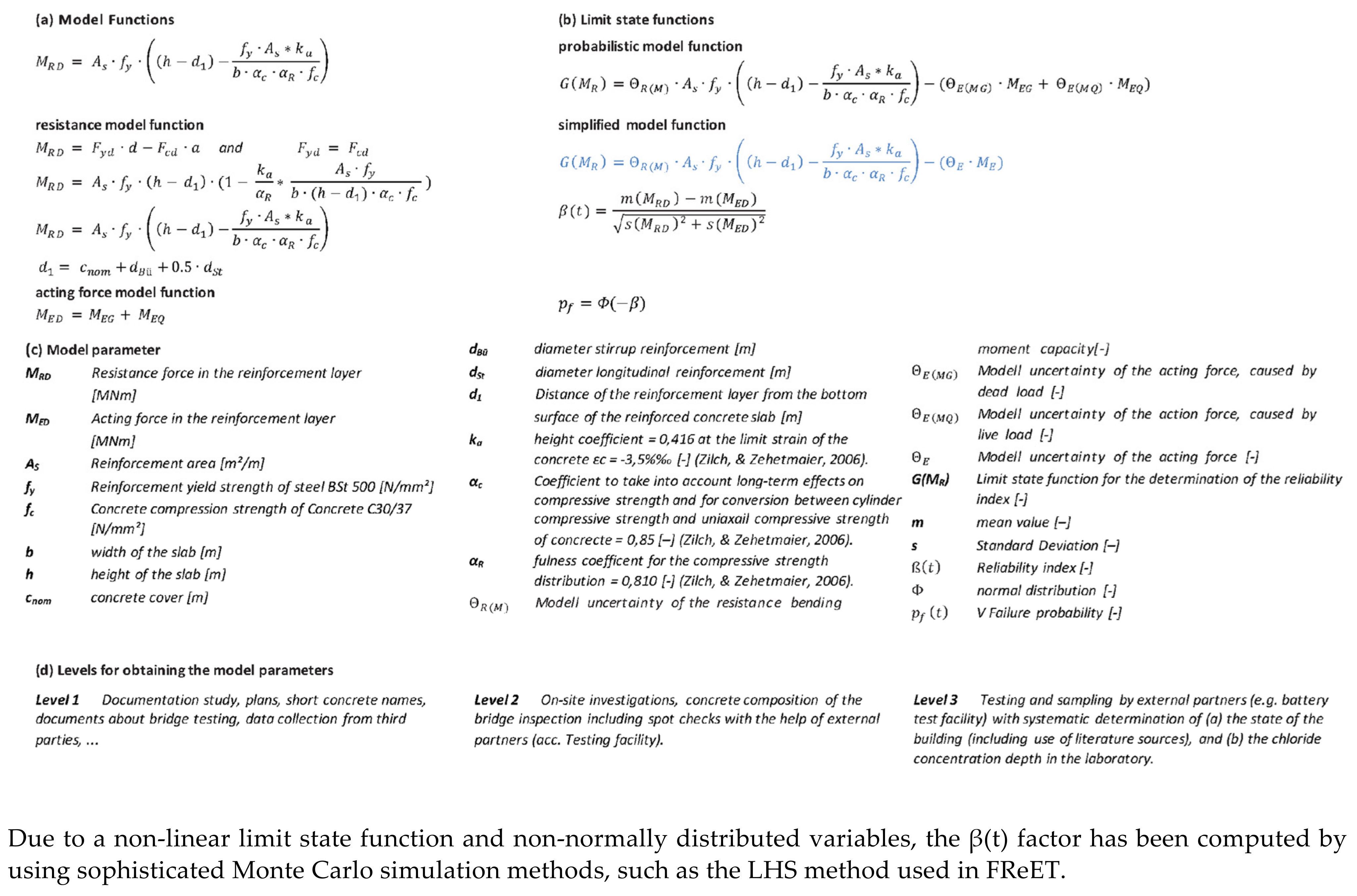
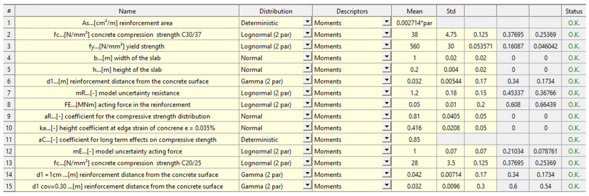
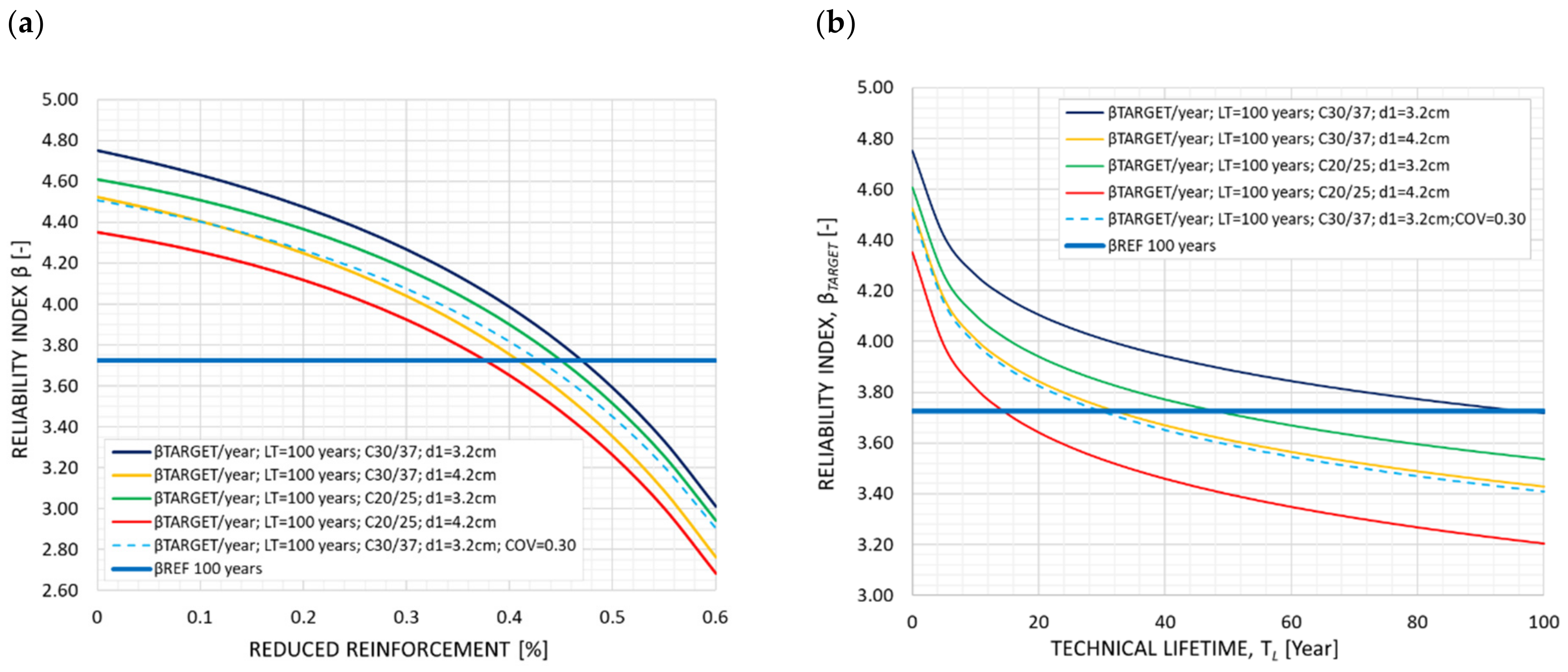
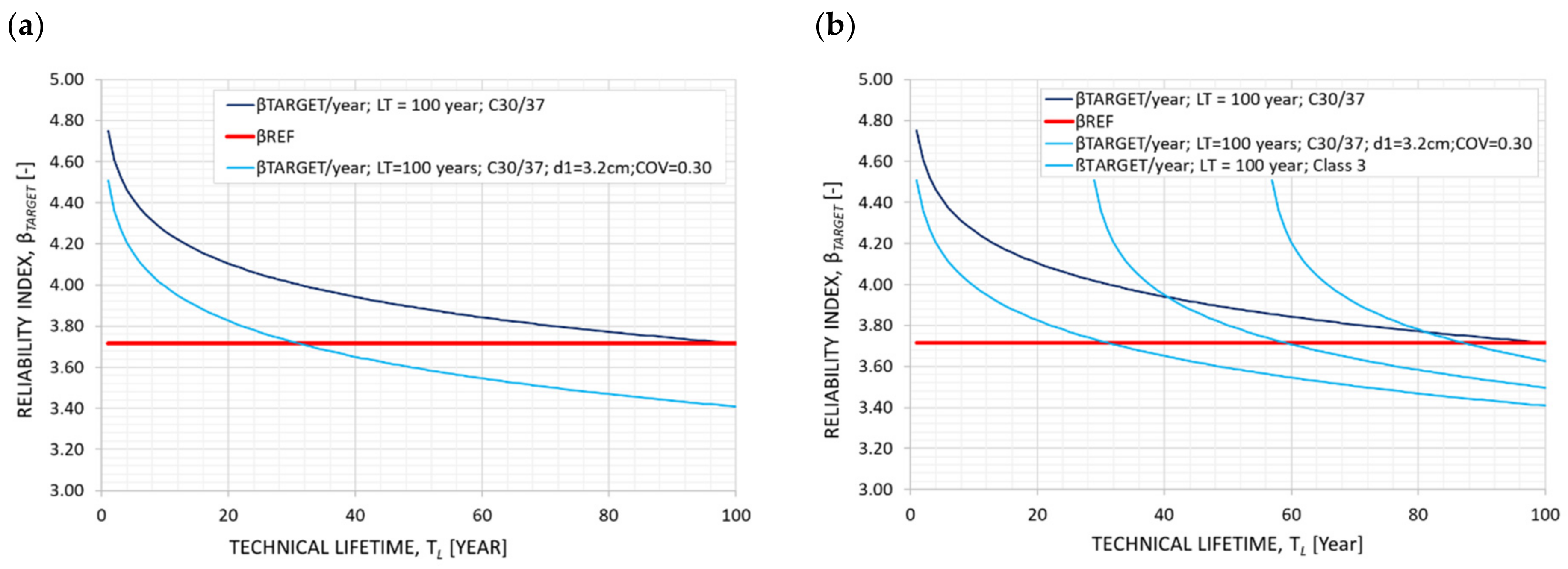
5. Case Study on Bearing Capacity

In this case study, a one-way-reinforced concrete slab was used, with a width of b = 1 m and a height h = 0.20 m. The calculation of the moment bearing capacity assumes a longitudinal reinforcement area of A_s = 27.14 cm²/m. The limit-state function (Equation (2)) is formulated with respect to the bending-tensile strength of the reinforcement on the ULS (ultimate limit state) level based on [41,42]. The geometrical dimension of the slab, the reinforcement area, the material properties and the applied load are elaborated on in the probabilistic analysis. The model uncertainty of the resistance bending moment capacity was characterised as 1.20, according to the JCSS Probabilistic Model Code [43]. The influence parameters addressed in this case are the static height of the reinforcement, depending on the reinforcement placement accuracy, and the loss of reinforcement action due to, e.g., corrosion and gradual bond loss as a result of an inadequate execution of the design. An additional influence parameter is the concrete class used, which also strongly affects the reliability assessment results.

Specifically, Figure 11a shows the basic function of the bearing capacity formulation, along with the complementary functions presented in [44]. The basic bearing-capacity function is transformed to a limit state function (Figure 11b) to be used as a basis for the definition of the β index, according to the classical Basler–Cornell approach, and it can therefore be used to define the failure probability (p_f). The necessary input variables, indices and parameters for the function of Figure 11a are presented in detail in Figure 11c. The models presented in Figure 11a,b and their input parameters can be obtained through various inspection levels, as shown in Figure 3d. As already mentioned in Section 4.1 and included in Figure 11 for consistency, a distinction can be made in the form of survey between the Level 1, Level 2 and Level 3 inspections.

Table 9. Model parameters of the bearing capacity model.

Variable Symbol	Unit	Literature and Background Information	Distribution *	Mean Value	Standard Deviation	COV
(1) MRD	(MNm)	[43,44,45]	-	-	-	-
(2) MED	(MNm)	[43,44,45]	LN	0.05	0.01	0.2
(3) AS	(cm2/m)	[43,44,45]	K	27.14	0.5428	0.02
(4) fy	(N/mm2)	[43,44,45]	LN	560	30	0.05357
(5.1) fc C30/37	(N/mm2)	[43,44,45]	LN	38	4.75	0.125
(5.1) fc C30/37	(N/mm2)	[43,44,45]	LN	27	3.5	0.125
(6) b	(m)	[43,44,45]	N	0.2	0.2	0.02
(7) h	(m)	[43,44,45]	N	1	0.004	0.02
(8.1) d1	(m)	[43,44,45]	G	0.032	0.0054	0.17
(8.2) d12	(m)	[43,44,45]	G	0.042	0.00714	0.17
(9) ka	(-)	[43,44,45]	N	0.416	0.0405	0.05
(10) αc	(-)	[43,44,45]	K	0.85	-	-
(11) αR	(-)	[43,44,45]	N	0.816	0.0208	0.05
$\left(12\right){\mathsf{\Theta }}_{R\left(M\right)}$	(-)	[43,44,45]	LN	1.2	0.18	0.15
$\left(13\right){\mathsf{\Theta }}_E$	(-)	[43,44,45]	LN	1	0.07	0.07

* Normal distribution, N; lognormal distribution, LN; constant, K; gamma distribution, G.

gives a general overview of the chosen input parameters that were used in the model function, with the respective literature sources in which the parameters are described. The table also presents the statistical model description of certain parameters (grey-highlighted area). In the analyses, the reinforcement area was taken as a constant variable, and it was multiplied by the parameters in the range of 0.4 to 1 to simulate the loss of reinforcement steel. The analysis was performed with two different types of concrete (C20/25 and C30/37), and for each type of concrete, the distance from the bottom of the slab to the reinforcement was varied between 32 and 42 mm. To calculate the limit-state excess probabilities and subsequently the reliability indices β, the software FReET was used and the first set of input parameters is shown in Figure 12.

Figure 13a demonstrates the development of the reliability index for a variation of reinforcement loss. It can be seen that the distance between the reinforcement and the concrete surface (d₁) is more important in terms of reliability than compression strength. As the reinforcement area A_s decreases, the influence of the concrete compression strength becomes less significant. For a concrete class C30/37 and d₁ = 32 mm (solid dark-blue line), the reliability index is β = 4.75, which corresponds to a failure probability of p_f = 1.01·10⁻⁶. For a lifetime of 100 years, the β_TARGET is reduced to 3.72, as seen in Figure 13b. For this assessment situation, and a loss of 45% reinforcement area, the β_TARGET would be critical for the flexural load-bearing assessment. For the same concrete type C30/37 but an increased distance between the reinforcement and the concrete surface with d₁ = 42 mm (solid orange line), a loss of 40% would already lead to the service life limit of β_TARGET = 3.72 after 30 years. On the contrary, a lower concrete class (C20/25) and the same distance between the reinforcement and the concrete surface d₁ = 32 mm (solid green line) would allow for a loss of 43% of the reinforcement area and the reliably index β_TARGET would be attained at 48 years.

In the baseline assessment and as shown in Figure 12, the COV for the positioning of the reinforcement is set to COV(d₁) = 0.17. For a COV(d₁) of 0.30, the reliability index without any loss of reinforcement drops to 4.52 (p_f = 3.07·10⁻⁶), with a notable consequence for the remaining expected service life, as shown in Figure 13a,b (dashed blue line).

The development of the system’s reliability with this change in the standard deviation in the reinforcement layer location (distance from the concrete surface), under the assumption of a lognormal distribution and the same concrete class (C30/37), is illustrated in Figure 14a. This represents a typical quality issue in construction, and the influence of quality on the structure’s reliability is reflected. Figure 14b shows that the system with reduced reliability, as the standard deviation in the reinforcement location needs to be updated more than two times throughout the asset’s lifetime in order to maintain the target reliability index for at least 100 years.

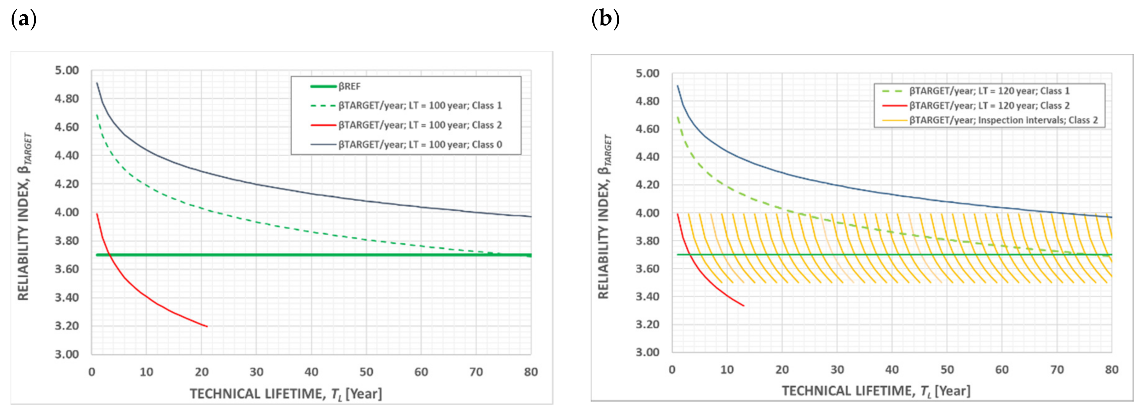
6. Case Study on Fastenings

Quality in fastening installation is known to have a substantial influence on the assembly’s load-bearing resistance and reliability, particularly for post-installed fastenings, which is also noted in the newly introduced Eurocode 2 part 4 EN 1992-4 “Design of fastenings for use in concrete” [46], see

Table 10. Excerpt from “Table 4.1—Recommended values of partial factors” from EN 1992-4:2018 [46].

Concrete Failure
Cone break-out failure, edge break-out failure, blow-out failure and pry-out failure	γΜc = γc * γinst. γc = 1.5a; see EN 1998 for seismic repair and strengthening. γinst = 1.0 for headed fasteners and anchor channels satisfying the requirement of 4.5 (in tension and shear), ≥1.0 for post-installed fasteners in tension; see relevant European Technical Product Specification, =1.0 for post-installed fasteners in shear.
Splitting failure	γΜsp = γMc
Pull-out Failure
Pull-out and combined pull-out and concrete failure	γΜp = γMc
a The values are in accordance with EN 1992-1-1.

. The design code is based on the typical partial factor design, while it considers that the partial safety factor for the resistance side is the product of the material safety factor γ_Μc familiar for concrete and the safety factor to account for the sensitivity to installation of post-installed fasteners γ_inst. The factor γ_inst is generally derived from standardised installation safety tests. The predecessor of EN 1992-4, namely the ETAG 001—Annex C [47], proposed the following values for the partial safety factor taking account of the installation safety of an anchor system as follows:

Tension loading

• γ₂ = 1.0 for systems with high installation safety;
•   = 1.2 for systems with normal installation safety;
•   = 1.4 for systems with low but still acceptable installation safety.

In many project specifications, the installers require training and certification. A typical procedure is presented in [48], while standardisation institutes provide detailed guidance for the installation of fastenings [49,50]. Notable failures with significant consequences have been attributed to design and installation errors, and it has also been reported that inspections could have helped avoid the incidents [51,52]. Site surveys have also indicated that the installation quality and the level of awareness for the exact installation procedures may strongly vary [53,54]. Inherent defects are also present during the production of fastening products, in the range of 2·10⁻⁵ [55], although factory QC processes may withhold most defective products from the market.

Based on test results for bonded anchors [56], the random variables are provided in

Table 11. Model parameters of the anchor pull-out probabilistic model; the range of values for the embedment depth equals the minimum and maximum boundary deviations of the variable, and it is equal to the standard deviation for the bond strength and the load.

Variable Symbol	Unit	Literature and Background Information	Distribution *	Mean Value	Range	COV	Distribution *	Mean Value	Range	COV
(1) Anchor diameter d	(mm)	-	K	16	-	-	K	16	-	-
(2) Embedment depth heff	(mm)	-	R	80	0.5	0.004	R	80	2	0.018
(3) Bond strength τ	(N/mm2)	[56]	LN	16.05	0.39	0.024	LN	15.25	0.41	0.027
(4) Load E	(N)	-	N	40,000	5000	0.125	N	40,000	5000	0.125

* Normal distribution, N; lognormal distribution, LN; rectangular distribution, R; constant, K.

for (a) an anchor with good installation quality (Class 1) and (b) an anchor with substandard quality (Class 2). The load is assumed from typical applications at 40 kN with a variation coefficient of COV(E) = 0.125. The worst-case scenario of hole cleaning (no hole cleaning) in tests led to a decrease in load bearing by 30%, which is roughly proportional to the added safety reserves represented by the installation factor of γ_inst = 1.4. However, this also leads to an increase in the standard deviation by a factor of 7.0, which automatically renders the reliability of the system below any acceptable level (β = 1.1; p_f = 0.135), and hence this case is not further considered. The random variables associated with substandard borehole preparation in the assessment below are taken with a multiplication factor of 0.95. For Class 1, and the results indicate a reliability index of 4.68, while for Class 2, although the differences are marginal, the results show a much lower reliability index of 3.99. Assuming an 80-year service life, the β_REF is assumed equal to the end-of-life reliability of the Class 1 system, equal to β₁₂₀ = 3.7, as shown in Figure 15. Consequently, for an 80-year lifetime of a Class 2 system, multiple inspections are needed in order to maintain the target reliability of 3.7, ideally every 3 years. In an idealised case, applying the mean values of Class 1 used as the deterministic input with an absolute absence of variation (Class 0) is also given in the graph for comparison. This set of parameters yields an origin reliability value of β₀ = 4.91.

7. Summary of Findings

In the carbonation analysis, it is made evident that the wrong selection of cement (CEM) type and the associated w/c ratio can reduce the component’s service life while an adequate selection of these parameters can increase the component’s service life. For example, although all investigated cases have a reliability index of the same orders of magnitude (between 4.27 and 4.66), assuming a target reliability index of β = 2.9, a service life of 50 years can be guaranteed for CEM I while the service life with a CEM III-based mix can reach just over 10 years. Inversely, for the same target service life, the CEM III component reaches a reliability index of only 1.59 for 50 years. With a variation of 5% in the w/c ratio of the CEM I mix, the service life of 50 years (β = 2.9) drops to only 27 years. Along the same lines, a chloride ingress analysis qualifies CEM III with an allowable exposure time of 50 years for a reliability index of β = 1.56, whereas structures with CEM I and CEM II are deemed to maintain this performance level for only 4 and 6 years of exposure, respectively. With regard to the load-bearing capacity of a one-way slab under flexural response and tolerances in the placement of reinforcement and its effective area, for a placement error (e.g., due to the lack of rebar support in the formwork) of only 10 mm, the estimated service life of the structure drops from 100 years to under 50 years. Finally, a minimal variation in the bond strength of the adhesive used, together with a common installation tolerance in the embedment depth, can reduce a typical bonded anchor’s service life from 80 years to only 3 years.

To counterbalance the significant loss of structural reliability, time intervals for periodic updating in the spirit of the fib Model Code 2020 are calculated. The inspection and updating intervals aim to maintain the reliability of the investigated systems above the reference value, which is estimated as the target reliability of a well-executed concrete specification or structural detail. These intervals were found to be 30 years in the case of the one-way slab and 3 years in the case of anchors. Depending on these results, a periodic adjustment procedure and the means used to perform this adjustment can be decided. This study distinguishes between three levels of updating the assessment parameters: documentation-based assessment, on-site investigations and inspections and systematic sampling (e.g., by using regular laboratory tests or monitoring).

8. Conclusions

In this paper, the structural reliability of typical engineering design situations is evaluated with regard to the structural component’s execution quality. In particular, it is shown on the basis of case studies that even marginal quality variations in the initial condition of the structure can dramatically affect the structure’s service-life duration. The strong sensitivity of the life-cycle reliability of structures and elements of QC and quality assurance at construction and along the service life of a structure is hence indicated. The quality criteria can be associated with structural reliability by means of the involved parameters’ statistical models, based on the novel methodology, using the reliability index β. This methodology was trialled on two realistic case studies of durability assessment (durability design for concrete carbonation and chloride ingress assessment), a typical flexural design for a one-way concrete slab and a design for a single bonded anchor in concrete. The method is applicable to all new concrete structures with on-site or off-site construction elements, particularly with special requirements in terms of life-cycle performance. However, although this concept was tested for each presented design situation, this study does not cover all possible aspects of advanced materials and the respective whole-life assessment and environmental influences. In future investigations, this concept can be applied not only to a wider range of modern civil engineering problems, such as construction materials under various environmental impacts, high- and ultra-high-performance concrete and advanced concrete composites in terms of resilience, durability and sustainability, but also extreme events, such as seismic actions, as discussed in [57,58,59,60,61,62,63,64,65,66,67,68,69,70].

As noted, marginal quality variations can lead to significant variations in the performance levels of the structure, for example, the residual service life. Considering the investigated cases, the reduction in service life can fluctuate from 20% to 95% of the envisaged target service life, which can translate to an equal loss of whole-life value of the asset. The monetary loss in this case can be represented by a reduced duration of the operational performance or by the inspection and upgrading activities. In all cases, the presented investigations affirm the importance of an adequate and effective quality management plan at the initial phases of a construction project, which is of minor expense but can lead to gain in terms whole-life costing and life-cycle performance perspective.

References

1. ISO 55000:2014; Asset Management—Overview, Principles and Terminology. ISO: Geneva, Switzerland, 2014.
2. Frangopol, D.M.; Strauss, A.; Kim, S. Bridge reliability assessment based on monitoring. J. Bridge Eng. 2008, 13, 258–270. [Google Scholar] [CrossRef]
3. Zambon, I.; Vidović, A.; Strauss, A.; Matos, J. Condition prediction of existing concrete bridges as a combination of visual inspection and analytical models of deterioration. Appl. Sci. 2019, 9, 148. [Google Scholar] [CrossRef] [Green Version]
4. Zimmermann, T.; Strauss, A.; Lehký, D.; Novák, D.; Keršner, Z. Stochastic fracture-mechanical characteristics of concrete based on experiments and inverse analysis. Constr. Build. Mater. 2014, 73, 535–543. [Google Scholar] [CrossRef]
5. Gehlen, C.; Schiessl, P.; Schiessl-Pecka, A. Background information on the DAfStb opinion paper on the implementation of the concept of performance-based design methods under consideration of DIN EN 206-1, Annex J, for problems relevant to durability. Beton-Und Stahlbetonbau 2018, 103, 840–851. [Google Scholar] [CrossRef]
6. Basler, E. Studies on the Concept of Safety of Structures. Ph.D. Thesis, ETH Zurich, Zurich, Switzerland, 1960. [Google Scholar]
7. Schneider, J. Introduction to Safety and Reliability of Structures; Structural Engineering Documents 5 (SED 5); International Association for Bridge and Structural Engineering (IABSE): Zurich, Switzerland, 1997. [Google Scholar]
8. Schneider, J.; Vrouwenvelder, T. Introduction to Safety and Reliability of Structures; Structural Engineering Documents 5-3rd reviewed and extended Edition; International Association for Bridge and Structural Engineering (IABSE): Zurich, Switzerland, 2017. [Google Scholar]
9. fib-International Federation for Structural Concrete. Bulletin 34: Model Code for Service Life Design; fib: Lausanne, Switzerland, 2006. [Google Scholar]
10. CEN-European Committee for Standardization. EN 1990: 2002-Basis of Structural Design (Eurocode 0); CEN: Brussels, Belgium, 2002. [Google Scholar]
11. ISO 13822:2010; Basis for Design of Structures—Assessment of Existing Structures. ISO: Geneva, Switzerland, 2010.
12. EN 13670:2009; Execution of Concrete Structures. CEN: Brussels, Belgium, 2009.
13. EN 1090-1:2012; Execution of Steel Structures and Aluminium Structures-Part 1: Requirements for Conformity Assessment of Structural Components. CEN: Brussels, Belgium, 2012.
14. FSV-Austrian Research Association for Roads, Railways and Transport. Guidelines and Regulations for the Road Sector: Supervision, Control and Testing of Civil Engineering Works-Road Bridges (RVS 13.71); FSV: Vienna, Austria, 1995. [Google Scholar]
15. fib-International Federation for Structural Concrete. Model Code 2010: Final Draft; fib: Lausanne, Switzerland, 2012. [Google Scholar]
16. Matthews, S.; Bigaj-van Vliet, A.; Walraven, J.; Mancini, G.; Dieteren, G. fib Model Code 2020: Towards a general code for both new and existing concrete structures. Struct. Concr. 2018, 19, 969–979. [Google Scholar] [CrossRef]
17. EN 12390-12; Testing Hardened Concrete-Part 12: Determination of the Carbonation Resistance of Concrete-Accelerated Carbonation Method. CEN: Brussels, Belgium, 2020.
18. EN 14630; Products and Systems for the Protection and Repair of Concrete Structures-Test Methods-Determination of Carbonation Depth in Hardened Concrete by the Phenolphthalein Method. CEN: Brussels, Belgium, 2006.
19. ISO 16204:2012; Durability—Service Life Design of Concrete Structures. ISO: Geneva, Switzerland, 2012.
20. CEB-European Committee for Concrete. Bulletin 238: New Approach to Durability Design: An Example for Carbonation Induced Corrosion; CEB: Lausanne, Switzerland, 1997. [Google Scholar]
21. CEB-European Committee for Concrete. Bulletin 152: Durability of Concrete Structures, State-of-the-Art; CEB: Paris, France, 1983. [Google Scholar]
22. CEB-European Committee for Concrete. Bulletin 182: Durable Concrete Structures, CEB Design Guide; CEB: Lausanne, Switzerland, 1989. [Google Scholar]
23. DAfStb-German Committee for Structural Concrete. Guideline for Improving the Durability of Exterior Reinforced Concrete Structures; DAfStb: Berlin, Germany, 1983. [Google Scholar]
24. DAfStb-German Committee for Structural Concrete. DafStb Guideline for the Curing of Concrete; DAfStb: Berlin, Germany, 1984. [Google Scholar]
25. von Greve-Dierfeld, S.; Gehlen, C. Performance based durability design, carbonation part 1–Benchmarking of European present design rules. Struct. Concr. 2016, 17, 309–328. [Google Scholar] [CrossRef]
26. von Greve-Dierfeld, S.; Gehlen, C. Performance-based durability design, carbonation, part 3: PSF approach and a proposal for the revision of deemed-to-satisfy rules. Struct. Concr. 2016, 17, 718–728. [Google Scholar] [CrossRef]
27. Gehlen, C. Probability-Based Service Life Design of Reinforced Concrete Structures–Reliability Studies for Prevention of Reinforcement Corrosion. DAfStb Bullettin 510; DAfStb: Berlin, Germany, 2000. [Google Scholar]
28. Ruixia, H. A study on carbonation for low calcium fly ash concrete under different temperature and relative humidity. Electron. J. Geotech. Eng. 2010, 15, 1871–1877. [Google Scholar]
29. RILEM-International Union of Testing and Research Laboratories for Materials and Structures. Corrosion of Steel in Concrete: Report of the Technical Committee 60 CSC, RILEM; Schiessl, P., Ed.; RILEM: London, UK, 1988. [Google Scholar]
30. Novák, D.; Vořechovský, M.; Teplý, B. FReET: Software for the statistical and reliability analysis of engineering problems and FReET-D: Degradation module. Adv. Eng. Softw. 2014, 72, 179–192. [Google Scholar] [CrossRef]
31. FREET (Feasible Reliability Engineering Tool). Publications. Available online: http://freet.cz/Publications.html (accessed on 20 April 2021).
32. DuraCRETE Consortium. Modelling of Degradation: Probabilistic Performance Based Durability Design of Concrete Structures; EU Project (Brite EuRam III) No. BE95-1347, Report No 4-5; Centre for Civil Engineering Research and Codes CUR: Gouda, The Netherlands, 1998. [Google Scholar]
33. fib-International Federation for Structural Concrete. Bulletin 76: Benchmarking of Deemed-To-Satisfy Provisions in Standards: Durability of Reinforced Concrete Structures Exposed to Chlorides; fib: Lausanne, Switzerland, 2015. [Google Scholar]
34. fib-International Federation for Structural Concrete. Bulletin 59: Condition Control and Assessment of Reinforced Concrete Structures: Exposed to Corrosive Environments (Carbonation/Chlorides); fib: Lausanne, Switzerland, 2011. [Google Scholar]
35. Zambon, I.; Vidović, A.; Strauss, A.; Matos, J. Use of chloride ingress model for condition assessment in bridge management. Građevinar 2019, 71, 359–373. [Google Scholar]
36. Zambon, I.; Vidović, A.; Strauss, A.; Matos, J.; Friedl, N. Prediction of the remaining service life of existing concrete bridges in infrastructural networks based on carbonation and chloride ingress. Smart Struct. Syst. 2018, 21, 305–320. [Google Scholar]
37. Šomodíková, M.; Strauss, A.; Zambon, I.; Teplý, B. Quantification of parameters for modeling of chloride ion ingress into concrete. Struct. Concr. 2019, 20, 519–536. [Google Scholar] [CrossRef]
38. Ferreira, R.M. Implications on RC structure performance of model parameter sensitivity: Effect of chlorides. J. Civ. Eng. Manag. 2010, 16, 561–566. [Google Scholar] [CrossRef] [Green Version]
39. EN 14629:2007; Products and Systems for the Protection and Repair of Concrete Structures-Test Methods-Determination of Chloride Content in Hardened Concrete. CEN: Brussels, Belgium, 2007.
40. EN 12390-11; Testing Hardened Concrete-Part 11: Determination of the Chloride Resistance of Concrete, Unidirectional Diffusion. CEN: Brussels, Belgium, 2010.
41. ONR 24008 (2014 03 01); Assessment of the Bearing Capacity of Existing Railway and Road Bridges. ASI: Vienna, Austria, 2014.
42. DIN 1045-1:2001-07; Concrete, reinforced and prestressed concrete structures-Part 1: Design. DIN: Berlin, Germany, 2001.
43. JCSS-Joint Committee on Structural Safety. JCSS Probabilistic Model Code; JCSS: Aalborg, Denmark, 2000. [Google Scholar]
44. Braml, T. On the Assessment of the Reliability of Concrete Bridges on the Basis of the Results of Structure Inspections. Ph.D. Thesis, Bundeswehr University Munich, Neubiberg, Germany, 2010. [Google Scholar]
45. Braml, T.; Keuser, M.; Bergmeister, K. Basics and Development of Stochastic Models for a Structural Reliability Assessment of Reinforced Concrete Bridges on the Basis of the Results from Bridge Inspection. Beton-Und Stahlbetonbau 2011, 106, 112–121. [Google Scholar] [CrossRef]
46. EN 1992-4; 2018 Design of Concrete Structures. Design of Fastenings for Use in Concrete (Eurocode 2–Part 4). CEN: Brussels, Belgium, 2018.
47. EOTA-European Organization for Technical Approvals. ETAG 001: Guideline for European Technical Approval of Metal Anchors for Use in Concrete, Annex C: Design Methods for Anchorages; 3rd Amendment; EOTA: Brussels, Belgium, 2010. [Google Scholar]
48. ACI-American Concrete Institute. Adhesive Anchor Installer Workbook; ACI: Farmington Hills, MI, USA, 2012. [Google Scholar]
49. BS 8539:2012; Code of Practice for the Selection and Installation of Post-Installed Anchors in Concrete and Masonry. BSI: London, UK, 2012.
50. German Institute for Construction Engineering. Instructions for the Installation of Dowel Anchors; DIBt: Berlin, Germany, 2010. [Google Scholar]
51. NTSB-National Transportation Safety Board. Highway Accident Report: Ceiling Collapse in the Interstate 90 Connector Tunnel at Boston, Massachusetts, July 10, 2006; NTSB: Washington, DC, USA, 2007. [Google Scholar]
52. Kawahara, S.; Shirato, M.; Kajifusa, N.; Kutsukake, T. Investigation of the tunnel ceiling collapse in the central expressway in Japan. In Transportation Research Board 93rd Annual Meeting; Transportation Research Board: Washington, DC, USA, 2014. [Google Scholar]
53. Grosser, P.; Fuchs, W.; Eligehausen, R. A field study of adhesive anchor installations. Concr. Int. 2011, 33, 57–63. [Google Scholar]
54. New Civil Engineer. Industry Fears over Fixings. Available online: www.newcivilengineer.com/latest/industry-fears-over-fixings-10-09-2015 (accessed on 15 January 2022).
55. Standring, P. Fastener and Fixings. A Consideration of Zero Defects. Available online: www.fastenerandfixing.com/technical/a-consideration-of-zero-defects (accessed on 15 January 2022).
56. Spyridis, P.; Walter, L.; Dreier, J.; Biermann, D. Laboratory investigations on the installation of fasteners in fiber reinforced concrete. In RILEM-Fib International Symposium on Fibre Reinforced Concrete; Springer International Publishing: Heidelberg, Germany, 2020. [Google Scholar]
57. Farzampour, A. Temperature and humidity effects on behavior of grouts. Adv. Concr. Constr. 2017, 5, 659–669. [Google Scholar]
58. Farzampour, A. Compressive Behavior of Concrete under Environmental Effects. In Compressive Strength of Concrete; Kryvenko, P., Ed.; IntechOpen: London, UK, 2019. [Google Scholar]
59. Chalangaran, N.; Farzampour, A.; Paslar, N.; Fatemi, H. Experimental investigation of sound transmission loss in concrete containing recycled rubber crumbs. Adv. Concr. Constr. 2021, 11, 447–454. [Google Scholar]
60. Chalangaran, N.; Farzampour, A.; Paslar, N. Nano silica and metakaolin effects on the behavior of concrete containing rubber crumbs. Civ. Eng. 2020, 1, 264–274. [Google Scholar] [CrossRef]
61. Liao, J.; Yang, K.Y.; Zeng, J.J.; Quach, W.M.; Ye, Y.Y.; Zhang, L. Compressive behavior of FRP-confined ultra-high performance concrete (UHPC) in circular columns. Eng. Struct. 2021, 249, 113246. [Google Scholar] [CrossRef]
62. Pan, B.; Liu, F.; Zhuge, Y.; Zeng, J.J.; Liao, J. ECCs/UHPFRCCs with and without FRP reinforcement for structural strengthening/repairing: A state-of-the-art review. Constr. Build. Mater. 2022, 316, 125824. [Google Scholar] [CrossRef]
63. Zeng, J.J.; Ye, Y.Y.; Quach, W.M.; Lin, G.; Zhuge, Y.; Zhou, J.K. Compressive and transverse shear behaviour of novel FRP-UHPC hybrid bars. Compos. Struct. 2021, 281, 115001. [Google Scholar] [CrossRef]
64. Ahmad, A.; Farooq, F.; Niewiadomski, P.; Ostrowski, K.; Akbar, A.; Aslam, F.; Alyousef, R. Prediction of compressive strength of fly ash based concrete using individual and ensemble algorithm. Materials 2021, 14, 794. [Google Scholar] [CrossRef] [PubMed]
65. Song, H.; Ahmad, A.; Farooq, F.; Ostrowski, K.A.; Maślak, M.; Czarnecki, S.; Aslam, F. Predicting the compressive strength of concrete with fly ash admixture using machine learning algorithms. Constr. Build. Mater. 2021, 308, 125021. [Google Scholar] [CrossRef]
66. Xu, Y.; Ahmad, W.; Ahmad, A.; Ostrowski, K.A.; Dudek, M.; Aslam, F.; Joyklad, P. Computation of High-Performance Concrete Compressive Strength Using Standalone and Ensembled Machine Learning Techniques. Materials 2021, 14, 7034. [Google Scholar] [CrossRef]
67. Farooq, F.; Nasir Amin, M.; Khan, K.; Rehan Sadiq, M.; Faisal Javed, M.; Aslam, F.; Alyousef, R. A comparative study of random forest and genetic engineering programming for the prediction of compressive strength of high strength concrete (HSC). Appl. Sci. 2020, 10, 7330. [Google Scholar] [CrossRef]
68. Farooq, F.; Ahmed, W.; Akbar, A.; Aslam, F.; Alyousef, R. Predictive modeling for sustainable high-performance concrete from industrial wastes: A comparison and optimization of models using ensemble learners. J. Clean. Prod. 2021, 292, 126032. [Google Scholar] [CrossRef]
69. Wendner, R.; Strauss, A.; Guggenberger, T.; Bergmeister, K.; Teplý, B. Approach for the assessment of concrete structures subjected to chloride induced deterioration. Beton-Und Stahlbetonbau 2010, 105, 778–786. [Google Scholar] [CrossRef]
70. Strauss, A.; Krug, B.; Slowik, O.; Novak, D. Combined shear and flexure performance of prestressing concrete T-shaped beams: Experiment and deterministic modelling. Struct. Concr. 2018, 19, 16–35. [Google Scholar] [CrossRef] [Green Version]
Figure 1. Ishikawa causal diagram with the analysis of causes and factors of material degradation.
Infrastructures 07 00024 g001
Figure 2. Quality assurance and technical service life. (a) Loss in lifetime and (b) monitoring or testing updating due to a reduced initial reliability index.
Infrastructures 07 00024 g002
Figure 3. Carbonation prediction model. (a) Mathematical formulations to assess concrete carbonation, (b) limit state function and reliability assessment formulations, (c) their basic variables and (d) the levels of inspection to obtain the respective parameter.
Infrastructures 07 00024 g003
Figure 4. Case studies of model parameters in software FReET used for (a) CEM I, (b) CEM II and (c) CEM III.
Infrastructures 07 00024 g004
Figure 5. (a) Carbonation depth vs. exposure time for CEM I, CEM II and CEM III and (b) reliability index vs. exposure time.
Infrastructures 07 00024 g005
Figure 6. Quality assurance and technical service life. (a) Loss in lifetime and (b) monitoring or testing updating due to a reduced initial reliability index.
Infrastructures 07 00024 g006
Figure 7. Chloride prediction model. (a) Mathematical formulations to assess concrete carbonation, (b) limit state function and reliability assessment formulations, (c) their basic variables and (d) the levels of inspection to obtain the respective parameters.
Infrastructures 07 00024 g007
Figure 8. Input parameters for CEM I, CEM II and CEM III assigned in software FReET.
Infrastructures 07 00024 g008
Figure 9. (a) Chloride concentration vs. exposure time and (b) reliability index vs. exposure time of CEM I, CEM II and CEM II for chloride concentration at the reinforcement level of 55 mm, according to [5].
Infrastructures 07 00024 g009
Figure 10. Quality assurance and technical service life for chloride ingress. (a) Loss in lifetime and (b) monitoring or testing updating due to a reduced initial reliability index.
Infrastructures 07 00024 g010
Figure 11. Bearing capacity prediction model. (a,b) Mathematical formulations, (c) their basic variables and (d) the levels of inspection to obtain them.
Infrastructures 07 00024 g011
Figure 12. Input parameters for the bearing capacity assigned in software FReET.
Infrastructures 07 00024 g012
Figure 13. (a) Development of the reliability index vs. the loss of reinforcement and (b) development of the reliability index over the lifetime of 100 years.
Infrastructures 07 00024 g013
Figure 14. Quality assurance and technical service life. (a) Loss in lifetime and (b) monitoring or testing updating due to a reduced initial reliability index.
Infrastructures 07 00024 g014
Figure 15. Quality assurance and technical service life. (a) Loss in lifetime and (b) monitoring or testing updating due to a reduced initial reliability index.
Infrastructures 07 00024 g015