Article

Surrogate-Based Calculation Method for Robust Design Optimization Considering the Fatigue Probability for Variable Service Loads of eBike Drive Units

1
Bosch eBike Systems, TU Ilmenau, Product and Systems Engineering Group, 98693 Ilmenau, Germany
2
TU Ilmenau, Product and Systems Engineering Group, 98693 Ilmenau, Germany
*
Authors to whom correspondence should be addressed.
Submission received: 23 November 2023 / Revised: 13 December 2023 / Accepted: 18 December 2023 / Published: 25 December 2023

Abstract

:
This paper proposes a robust design-optimization approach for eBike drive units that incorporates the highly variable driver-dependent load collectives and system conditions into a fatigue calculation. In an initial step, the relevant influences and loads on the investigated system are examined and reviewed in relation to the current normative requirements. From a methodical viewpoint, this paper presents a surrogate-based simulation-based approach to assess reliability across the entire geometry according to a probabilistic fatigue calculation. The probabilistic evaluation considers the several measured load collectives of different drivers and driving scenarios to enable a robust and type-oriented bike design. In addition to methods of fatigue calculation, this approach also includes common methods of order reduction and reliability-based design optimization. To avoid additional uncertainties in the calculation, this approach considers a complex critical-plane-based multiaxial-fatigue calculation to correctly evaluate the multiaxial and non-proportional stress state across the whole geometry. A data-based surrogate model that supports the fatigue calculation by predicting the load across the given uncertainties is the key to the efficient assessment of the service life of the eBike. Lastly, the identified uncertainties in the design of eBike drive units are investigated and evaluated by this method.

1. Introduction

In recent years, eBikes have become increasingly popular and have come to represent a significant percentage of all bikes used across bike categories. Due to the novelty of the product and a fast-growing market, engineers are striving to rapidly improve the design and functionality of eBike engines and batteries. The general focus is this on, e.g., extended range, supporting torque and power density, as well as on improving engine control and riding experience to stay competitive. As the bicycle industry has historically been only component-oriented, eBike engines, which are now highly complex mechatronic sub-systems of the eBike, are considered standard components. Therefore, they should fit into any bicycle system regardless of the mounting position and application, which makes it necessary to focus the design process primarily on the reliability of the product and a robust design. This factor is especially relevant in the category of middle engines or so-called drive units (DUs), which replace the classic crankshaft and act as an interface between the pedals, the rider and the bike frame by providing support for the drive torque. For this purpose, this compact mechatronic system consists of a sensor system that detects the rider’s torque, a control-and-power electronic system that applies additional engine torque via a multistage gearbox and a free-wheel system to the crankshaft in relation to the desired level of assistance. An example of such a DU can be seen in Figure 1.
Due to this integration of this mechatronic system as an interface between the pedaling forces of the rider and the bicycle frame, the DU (as shown in the simplified hierarchical product structure of the eBike in Figure 2) is subject to external loads from the rider that are influenced and transmitted by parameterizable parts of the eBike and DU system, in addition to the internal loads from the motor and gear transmission. One examples of these influencing parameters is different crankshaft geometries, which affect the leverage of the pedal forces and thus have a strong influence on the DU loading. Comparably, different frame stiffnesses and mounting positions apparently influence the DU load. For consistency in nomenclature, these factors are classified as:
  • eBike-system-dependent parameter like the frame stiffness, mounting angle and geometry of the crankset and chain blade.
  • DU-dependent design parameters like the geometry and assembly of the housing and gears.
  • Loads consisting of driver-dependent dynamic pedal loads and DU-internal thermal and mechanical engine and gear loads, as well as static loads or residual stresses from assembly and manufacturing.
With respect to the loads, tremendous uncertainties must be considered in the design of the DU. These uncertainties are mainly caused by the expected variety in driver-dependent loads across users and driving scenarios. This variance in loads is increased by the case distinction of motor-assisted and non-assisted operation and the associated internal thermal and mechanical loads on the DU. Additional sources of uncertainty originate from assembly and manufacturing tolerances and influence the static loading of the DU.
As the current normative requirements are derived from conventional bicycles, they do not consider effects of the additional engine, which potentially causes higher torques, as well as thermal or mechanical loads on the DU. Furthermore, these requirements are set only at a component level, neglecting the influences of the integration of the DU into the overall eBike-system [3,4]. Overall, it can be questioned whether the current normative requirements can account for the variety and uncertainty of these loads and the given dependencies on all the parameters across the whole eBike system, which results in challenges in the development and verification of eBike DUs [5,6].
To investigate and assess the gap between the state-of-the-art requirements for the DU and the requirements in connection with potential use-case scenarios, fundamental studies were performed to determine real load collectives, the influence of the bike frame, DU internal loads and additional bike components on the load on the DU. These investigations show that the current normative requirements do not cover the whole load spectrum that can be observed during eBike use-case scenarios [5].
Consequently, for the DU design it is essential to quantify the impact of these load and parameter dependent uncertainties arising from the required variability of the bike industry with regard to the durability and a required service life of the DU to assure their application. Therefore, the objective of the Robust Design approach is based on a reliability constraint and aims at a probabilistic assessment of fatigue damage for all potential superpositions of the potential loads, all variants of eBike and all DU parameters.
To consider and incorporate these uncertainties even in the early stages of the product design process, a simulation-based approach of Robust Design and fatigue calculation should be developed. Simulations provide a simpler and therefore more cost-effective and faster adaption of load and parameter combinations, as well as an easily attainable evaluation of stress and strain values necessary for reliability evaluation.
Against this background, the objective of this paper is to develop a simulation-based method for the Robust Design, optimization and validation of products subjected to many uncertainties and highly variable load collectives, like the eBike DU. In view of the variable loads, the focus of robust optimization lies in a design that is resistant to fatigue and that performs well in a service-life assessment. To reduce the computational cost, which is typically the biggest impediment to industrial and practical applications of Robust Design methods, the development and validation of a feasible simulation-based calculation procedure based on reduced-order modelling techniques and a data-based surrogate model is discussed. To adequately account for the multiaxial and non-proportional loads in a cycle-based fatigue assessment, further methods incorporating fracture mechanics and the fatigue calculation are included in the computation chain.
The housing of the DU, which can be seen as the key element interfering with all further components of the DU and the overall eBike system, will be used as the research subject for the reliability-based Robust Design approach. Finally, the deviations between the existing normative and component-based requirements are determined in relation to the load that can be realistically expected in different applications of DUs across all bike types.
For this purpose, the following research questions are addressed and discussed in this paper:
  • Which parameters and loads need to be considered in a reliability-focused Robust Design process for eBike Drive Units?
  • How can a fast-computing simulation model be formed that includes the fatigue and service-life calculation and considers the uncertainties of the diverse load collectives and influencing parameters?
  • How can a cyclic multiaxial-fatigue calculation based on existing load collectives be integrated into a simulation-based reliability-based optimization approach?

2. State of the Art

This chapter presents the essential insights of the bicycle industry and the currently established and applied normative requirements. Additionally, the fundamental ideas and existing methods for simulation-based Robust Design and surrogate-based simulation are explained. Subsequentially, the most important steps of a fatigue calculation are explained.

2.1. Normative Requirements for eBikes

With the introduction of eBikes, previously existing normative requirements for conventional bicycles, which consist of component tests, were transferred to eBikes and their components. These requirements are described in [3,4] and defined on a component level by specifying load cases and boundary conditions for the testing of key components of the bicycle. These components include, for example, the frame, the wheels, the brakes, the handlebars, the saddle, the fork and the crankshaft, whose requirements have been transferred to the entire DU in the case of the eBike. Regarding the safety of mechanical components, the normative requirements of the eBike DU consist of two test variants that represent an exclusively vertically-acting cyclic pedal force for a specific crank angle (see Figure 3). The two variations consist of applying a pedal force (Fp) up to 1800 N either alternately to the right and left in a motion similar to normal cycling, or simultaneously, which simulates the load imposed by the rider’s weight in e.g., downhill riding situations. The magnitude of the force is thereby varied depending on the type of bicycle. To conduct the test, the DU is attached to a bracket that is not further specified. In the variant of alternating pedal forces, the resulting torque is absorbed by a fixed chain. The target cycle number that must be withstood to pass both tests again varies depending on the type of bicycle and the test variant. For further details of this normative test, such as the exact number of cycles and load specifications of individual bicycle types, please refer to the standard itself [3].
Regarding the bike frame, several load situations are defined, such as forces on the saddle, pedaling forces and loads on the wheel axis due to uneven surfaces or braking maneuvers [4]. Simplified boundary conditions are given for the bearing of the frame on the wheel axles. These boundary conditions can be derived from the counter-torque of the rider on the handlebars and the two contact points of the tires with the ground (see Figure 4). The required numbers of cycles and amplitudes depend on the type of bicycle.
Comparable simplified test scenarios, which allow testing of individual bicycle components under a constant amplitude, which is presumably based on an estimated worst-case scenario, potential worst-case scenario and respective boundary conditions, can be found for other components of the bike.
The different loading situations of the frame can be considered as matching counterparts to the individual loading situations of the other bike components that are linked to the frame, like the saddle or the handlebars. Hence, specific definitions of the relevant range of requirements for components besides the DU can be restricted to the frame, as that is the only part directly connected to the DU. From the perspective of robust DU design, however, it must be questioned whether separate consideration of the DU and the frame is possible. The following two influences and load types must be distinguished:
  • Determination of the forces that result from external loads on the frame and that are transferred to the DU.
  • Characterization of the influence of DU mounting on different bike-frame geometries and stiffnesses or on a uniformly stiff testrig on the loading situation.
Regarding the pedal load, it is doubtful that the uniaxial cyclic load of the normative requirement is comparable to the pedal force loading seen in real-life bike applications. This normative load is especially questionable in the light of a previous study on existing pedal-force measurements, which showed a considerably more complex picture of the human pedal cycle [7,8,9].
Significant observations related to this question are explained in [8,9]. Those studies describe the relevant proportions of pedal forces in all three Cartesian coordinates. Such an approach is only logical when considering that riders should want to apply the highest possible tangential force to increase their pedaling efficiency. Therefore, multi-axis pedal loads should be expected. Likewise, different proportions of applied pedal force, generated torque and the associated chain force can be anticipated. The study of [7] revealed clear differences in pedal-force measurements for different riding situations and riders, with resultant forces of up to 2000 N and individual force-to-weight ratios of up to 2.9. Transferred to the normative requirements discussed above, these measurements show potentially higher forces and, more importantly, confirm the assumption of individual cycling motions and pedal loads. Furthermore, it should not be forgotten that in the case of eBike DUs, the distinction between engine-assisted and engine-unassisted driving and the associated thermal and mechanical loads increases the variance in the load collective, although this variance is not even considered in the normative requirement. Therefore, the question arises of what kinds of loads and variations due to different riders, riding scenarios and DU assistance need to be considered in Robust Design. With regard to Robust Design for a certain service life, the transferability of the existing test, which is performed at constant amplitude, compared to the obviously multi-axial and variable amplitudes of real service loads, must be examined.

2.2. Robust Design Based on Simulation Methods

2.2.1. Robust Design and Design of Experiment

In the field of engineering, design robustness is a widely used term and condition that generally intends to minimize the sensitivity of a product function (or other product properties) to certain changes through operational or environmental parameters [10]. This perspective has origins in the ideas of Taguchi [11], who proposed an experiment-based approach to investigating the effects of “noisy” or statistically scattered parameters in relation to their impact on a targeted functionality of a product. Thereby, Taguchi defined the terms of controllable parameters that can be deterministically set by the designer, as well as of noise parameters, which cannot be controlled but can be described by a probability density functions, as they underlie statistical variance. Based on these definitions, Taguchi’s approach aimed at setting of the controllable parameters in such a way that the variations in the noise parameter do not affect the function of the product and have minimal impact on it [12].
Driven by this basic concept, the methods of DoE (Design of Experiments), as well as the definition of the uncertainties of a system, are elementary components of Robust Design. In this context, DoE methods are mainly used to efficiently explore the outcome of potential parameter combinations while also considering statistical variations.
Regarding uncertainties, different categories exist and must be considered differently in the design process. Here, one of the most common classifications in the literature is the division into aleatoric and epistemic uncertainty. Epistemic uncertainty is understood as a lack of information and can therefore be reduced by obtaining more information, e.g., through a DoE approach or more accurate measurement methods. Aleatory uncertainty, on the other hand, is often caused by inherent statistical variability and can be characterized by an empirical quantity; it is consequently the most decisive factor in Robust Design [13].
Especially when robustness is considered in relation to the reliability and safety of the product, an accurate evaluation of aleatory uncertainties arising from the environment, the system and user behavior is of enormous importance [14].
This evaluation is particularly important because a consideration of the robustness should be integrated as early as possible in the design process to enable the best possible responses to statistical influences. In practice, however, this variation is often considered only in later stages of the product-design process, when most design parameters are already fixed. Thus, clearly, fewer possible combination must be considered and computed. Thus, possible optimizations are voluntarily given up in order to reduce computational and testing efforts [14].

2.2.2. Simulation in the Context of Robust Design

For the representation of uncertainties in optimization approaches with regard to reliability, several methods in the field of Reliability-Based Design Optimization (RBDO) have been published in recent years [15]. Thereby, the key idea of optimization problem, minimizing a cost function dependent on a vector of design parameters, was extended to include statistical scattering that needs to be evaluated based on a probabilistic constraint regarded to a limit-state function. As the name would already indicate, the limit-state function is a function of all random variables that describes the failure criterion for the RBDO. For optimization approaches incorporating component safety, the limit-state function is often described by static variables like the maximum stress or strain [15,16,17]. Most of these methods are based on a double-loop principle, with one loop solving the probabilistic reliability analysis and the second loop dealing with the structural optimization [15,17].
According to [15], the methods used can be divided into gradient-based analytical and numerical-sampling-based methods. The most commonly used gradient-based method is the First Order Reliability Method (FORM), which approximates the limit-state function (defined by the scattering variables) by a linear first-order Taylor series expansion to identify the most probable point of failure and its probability. Further information about this method and its extensions to e.g., second-order approximation or different and non-Gaussian-distributed random variables can be found in [15,17,18].
The greatest advantage of this method is the low computing time, which is particularly evident in analytically solvable explicit problems. Also, for implicit problems, the FORM method can efficiently provide results in combination with a numerical simulation determining the derivatives of the limit-state function, such as the FEM simulation.
This advantage can be observed using simple academic examples in e.g., [15,19,20,21]. However, there are also severe limitations to this method, which particularly affect nonlinear limit-state functions with multiple potential error domains. Consequently, sampling methods are more suitable for these applications, although they are associated with significantly higher computational costs. To avoid errors due to the disregarding of these limitations, the sample-based simulation approaches of RBDO, alongside some hybrid approaches (as in [16]), have become well established for practical designs.
These simulation-based approaches are based on sampling methods such as the Monte Carlo method to represent the variation in the scattering parameters in order to describe the probabilistic changes in the respective fatigue conditions. As MC sampling operates by selecting from distribution functions of individual parameters, it provides little variance and requires a large number of computations to achieve sufficient coverage, which raised the demand for more efficient sampling methods. Widely used alternatives are space-filling approaches like Latin Hypercube Sampling (LHS), which aims to cover every part of the cumulative density function equally, or adaptive sampling strategies, which iteratively and dynamically updates sampling density as the simulation proceeds [18,22].
Further difficulties arise with both approaches in their application to time-dependent problems, which are usually caused by dynamic loads or decreasing material and component properties, e.g., due to corrosion [17,23,24]. The limit-state function can be described by time-variable parameter distributions and time-invariant parameters. This approach gives rise to the main problem for the calculation of the reliability via to the additional dimension introduced by time variance. Therefore, several methods of RBDO have been developed to address time-variant optimization targets. With regard to analytical approaches, a number of methods, like outcrossing and the extreme-value-based methods, were proposed. These methods mainly affect the discretization of the time course in order to calculate individual time periods as time-invariant cases by existing methods like FORM. Overall, in the practical application of time-variant problems, sampling approaches based on simulation have become increasingly established [17,23,24].
Nevertheless, the application of simulation-based methods to more complex practical industrial problems is usually difficult and limited due to the enormous computational effort required [18]. To minimize exactly this computational effort in the optimization of robust products with increasingly complex high-fidelity simulation models, the use of surrogate models and so-called surrogate-model-based design optimization has become an established practice in product development [25,26].
In this case, the primary purpose of the surrogate model is to replace the computationally expensive simulation involved in numerical high-fidelity models, such as FEM-simulation, with less computationally expensive numerical, analytical, or statistical models.

2.2.3. Order-Reduction Approaches and Surrogate Modeling

Overall, there are different approaches to the simplification of highly detailed physical models. Due to the basic principle of reducing model complexity, the term “surrogate modeling” is heavily linked with order-reduction methods and order-reduced modeling techniques. According to [27], these methods for order reduction and generation of a surrogate model can be classified into three main types: projection-based reduced models, hierarchical models and data-fit models.
Projection-based models are typically defined by simplified mathematical relationships derived from the high-fidelity model. Examples include physically-based analytical equations, the results of a spectral or modal analysis and decomposition and principal component analysis.
In contrast, hierarchical surrogates, also called variable-fidelity models, are derived from simplifications of the higher-fidelity models by simplification of physics-based relationships. Transferred to the example of an FEM simulation, this approach would include a coarser discretization, other element orders, or relaxed solver tolerances. Data-fitting surrogate models are instead non-physically-based approximations based on a relatively small number of coherent input and output data, which are calculated by few of the expensive high-fidelity calculations [28]. Consequently, the formation of this type of surrogate model can also be regarded as an advanced type of post-processing [29]. However, this approach has the disadvantage that, due to the absence of a physical reference, reliable results can be expected only for an interpolation task inside the given parameter space [27]. Nevertheless, this method has already shown enormous potential for the exploitation of a known parameter space, with the following references given as examples [30,31,32,33].
To perform a suitable approximation of the system behavior based on a small number of input-output combinations, the use of data-fit surrogate models is again inevitably linked to appropriate sample selection and DoE methods. This approach requires detection of local changes in the target output throughout the entire input-parameter domain, which is particularly difficult for multidimensional data sets because the distances between the data points increase exponentially. This method thus demands an enormous amount of sample data [26]. This problem is therefore generally known as the curse of dimensionality [34].
For the previously described reasons, space-filling sampling or adaptive and actively expanding sampling methods, rather than classical factorial or fractional factorial DoE methods and MC sampling, have been established for the formation of surrogate models [29,35]. For further information on sampling methods, readers are referred to [25,35].
For the creation of data-fit-based regression models, a variety of methods with different methodical approaches and levels of complexity have been developed and established in recent years. A general overview of these methods can be found in the work of [28]. Here, different analytical and stochastic regression methods like the Respond Surface Method and Kriging, as well as more modern machine learning methods based on decision trees and neural networks, are discussed and explained. Despite the different mathematical and logical operations that characterize each of these methods, they all have in common that they need to be trained by a suitable strategy.
The most commonly used training strategy with regard to the generation of data-based surrogate models of physical simulation data is the so-called supervised learning method. This method is based on combined input and output data sets, which are taken from measurements or simulations. Subsequentially, the data set is divided into training, test and, in some cases, additional validation data. Then, training occurs via an optimization loop to adjust and weight the model parameters of the selected model type to minimize the error between the surrogate model’s prediction for a given set of input data and the output data [36]. To describe this model prediction error, typical metrics like the root mean square error (RMSE), the relative and absolute error, or the R 2 value are used as general measures of regression quality.
To maintain the robustness of the model and to prevent overfitting or memorizing of the input-output correlations in the training data, the unseen data from the test split are also integrated into the optimization loop during training. To prove the independence of a data sample, additional comparisons with further validation data or a certain number of different data splits within cross-validations are performed. Cross-validation is a technique wherein the original training data set is split into k equal parts. Training is then performed for several runs of k − 1 different parts, while testing is performed on the remaining kth part of the data. This approach thus guarantees independence from any particular data pair. Besides the selection of the input data, the quality of the surrogate model depends on the choice of the so-called hyperparameters, which describe, e.g., the structure or the learning procedure of the surrogate model.
As these hyperparameter settings drastically influence the performance of the model, their adjustment is crucial for the comparison of different model types. Aside from the influence of these settings on model performance, the need for their adjustment also implies that different model types are only comparable if they possess equally adjusted hyperparameters. When comparing different model types, a setting of the hyperparameters equally adapted to application to the use case and the data set is crucial. In the following section, commonly used model types for data-based surrogate models and supervised-learning algorithms will be addressed briefly [37].

Artificial Neural Network

The architecture of Artificial Neural Networks (ANN) is inspired by biological functions found in the brain or nervous system and transferred to mathematical and numerical operations to process and assess data. Their general structure consists of several layers with interconnected neurons (depicted in Figure 5). Data are processed from an input layer throughout several hidden layers to calculate probability values for neurons in an output layer. These values constitute the basis for the model’s prediction. To perform these calculations, connections with parameterizable weights, activation functions and a certain bias are formed between neurons of different layers [30,37].
For a supervised-learning algorithm, ANNs are trained in the so-called backward propagation, which works retrospectively from a given input-output dataset. Subsequently, forward propagation can be used for a trained model, starting from the input data to determine the output values based on probability. Throughout the training process, the entire training dataset is evaluated iteratively over multiple training cycles (epochs), repeating backward propagation in separate batches to fit the training parameters. This fit is driven by an optimization algorithm in which a loss function based on error metrics, such as the RMSE or MSE, should be minimized. Thereby, limiting the maximum possible adjustment of the weights per cycle by imposing a learning rate helps to prevent instabilities in the optimization. As a result, the performance of the ANN depends significantly on the model or on hyperparameters like the chosen structure (neurons and number of layers) of the mathematical approach function and on the training parameters (learning rate, batch size, epochs) [28].

Tree-Based Regressors

Decision trees are one of the most-used model types for machine learning. Reasons for their popularity include their straightforward structure, their robustness against noise and their good ratio between performance and computation time. In addition, they are universally applicable due to the variability of processing nominal, numerical and text-based data independent of missing or redundant data [38]. The basic principles of tree-based models are the partitioning of the feature space and the fitting of a simple model or constant for the output of this partition. Based on the outcome of those steps, a decision tree can be built on simple Boolean decisions regarding the partitioned feature space (see Figure 6) [37].
One of the most-used model types is the Random Forrest (RF) model, which was proposed by [40], wherein several uncorrelated decision trees are built by bootstrap aggregation, which generates multiple trees with a random split of the training data through independent and individual training routines. For application to unseen data, the output values of all these trees are aggregated to depict the model output value in the form of the average value (for regression tasks) or the majority of votes (for classification).
Although the creation of multiple decision trees is computationally intensive, it minimizes the variance of individual trees and helps to prevent overfitting of the model by the “Law of Large Numbers” and the randomness of the tree building, which explains the robustness that is the trademark of the Random Forrest algorithm. In comparison to the simultaneous generation of decision trees in the RF, gradient-boosting algorithms like XGBoost (XG) grow decision trees sequentially to minimize the loss function of the model with each new tree while keeping the model size and tree number as small as possible [41]. To achieve this minimization rapidly, the gradient of the loss function with the previous model output is determined to generate the next data split. This potentially increases learning power by reducing computation time and improving performance at the expense of robustness and vulnerability to overfitting [39].
The decisive hyperparameters of the tree-based algorithms are the maximum number, depth and width of the decision trees, as well as the sample selection for the training data. Additional parameters can be defined for the process of gradient boosting. The initial claims of very good results with reasonable computational effort can also be confirmed by the benchmark investigations of [42], which show a generally good performance in significantly less training time for tree-based regressors compared to deep learning approaches in the form of neural networks for heteroscedastic tabular datasets. These studies also demonstrated the good performance of the RF and XG models for both regression and classification.

2.3. Fatigue Calculation

As a consequence of the trend towards light-weight design and the additional demands of minimizing costs and time-to-market intervals, product safety and reliability are of immense and growing interest for engineering designers. For that reason, the amount of research in the field of fatigue calculation and reliability is steadily increasing [43].
However, a distinction must be made between the experimental test-based determination of fatigue strength, which is mainly carried out in the final phase of the development process for the validation of the design, and the fatigue calculation done during the design phase of the product. The latter is usually based on simulation data evaluated in a local concept, where fatigue is evaluated at a specific area of the geometry using (estimated) material behavior. Given the focus of this work on robust optimization, the simulation-based calculation of service life is discussed here.
The origins of fatigue calculation for components made from metallic materials were defined by Wöhler, who discovered that while high loads can cause the static failure of structures, lower but cyclic loads can also lead to structural failure and fatigue. To discover material-specific fatigue behavior, Wöhler used experimental methods to characterize different materials and loads. Now, practical fatigue calculations are still based on empirical tests of specified geometries and loads to define the material limits for cyclic loads at different amplitudes. These tests are then combined to form the S-N-Curve (see Figure 7), which represents the number of cyclic loads of a certain load type and amplitude that result in the fatigue of the component [44].
This general information regarding the material can then be used for a comparison with calculated or measured loads of the investigated design to estimate its service life, which can be considered to be the most important outcome of fatigue calculation. To better subdivide the wide range of amplitudes and material-dependent fatigue properties recorded in the SN curve, the diagram for metallic materials is divided into three sections:
  • low-cycle fatigue, representing material behavior with plastic deformation;
  • high-cycle or very-high-cycle fatigue, representing material behavior with elastic deformation;
  • finite life, representing permanent durability.
Typical loads for these assessments are tension, compression, torsion and bending loads that are applied with different constant mean loads or ratios in the range between a fully reversed alternating or pulsating profile [46]. This ratio is important, as it characterizes the mean stress level of the cyclic loading, which can have a significant effect on the fatigue behavior, depending on the loading situation and material type. This influence can generally be visualized by the Haigh diagram, although multiple models have been proposed to describe it [46,47]. Besides the load type and the material, several other influences of fatigue behavior must be considered to allow fair comparison of the load conditions and data-based prediction of the service life. Further examples include the hardness of the material, corrosion effects and the surface roughness or finish, which is an important factor in the nucleation of microcracks. Likewise, the effect of stress gradients, occurring in the wake of residual stresses or notch geometries, must to be addressed in the comparison. To save experimental costs, these additional factors are usually not taken into account during measurement of the SN-Curve and are subsequently adjusted by additional correction factors [46,48].
Thus, not every amplitude or sample is inevitably and directly comparable using the SN-curve, but if they are not, they can be transformed to that end. For the evaluation of the desired service life, however, cumulative information on uniaxial loads at constant amplitudes must be transferred to variable amplitudes of real load spectra and complex load conditions from superimposed load channels.
As real loads are usually not uniaxial and of constant amplitudes and R-ratios, the problem arises that comparison with the material limits of the SN curve for basic loads can no longer be carried out directly. In practice, several superimposed load channels and real component geometries result in complex multiaxial stress states and loads, and these combinations have different amplitudes depending on their load collective. In such cases, the goal is to convert the calculated load to a reference value comparable with the values on the SN-curve.
In general, strength hypotheses based on the idea of assigning a damage-equivalent uniaxial load to each multiaxial stress state can be used to determine fatigue damage under multiaxial loading. First, this equivalent stress drastically reduces the complexity of the three-dimensional stress state. Second, it allows the calculation of fatigue life based on the reference and fatigue limits for uniaxial test loading. Here, the equivalent stress is usually compared with a typical SN curve for the material to predict the damage associated with the load under consideration [46].
In the case of multiaxial loading, the separation into proportional and non-proportional load components is of great importance. This is because non-proportional changes result in a rotation of the principal stress system, which of course requires a different analysis. In this case, common equivalent-stress theories such as von Mises or Tresca [47] are not applicable. This distinction and the selection of the correct calculation model is particularly relevant since experimental studies have shown significant differences in fatigue behavior between non-proportional and proportional multiaxial loading, which is schematically shown in Figure 7 [45].
Therefore, when calculating non-proportional loads, the entire load time sequence and its effects must be considered and different types of strength hypotheses must be utilized to account for these effects. Similarly, the simple scaling of the amplitude with respect to the single load signal, which is often used for proportional variable amplitude loading, is not recommended. Further information on this recommendation can be found for example in [48].
In recent years, several proposals have been made concerning strength hypotheses to determine an equivalent stress for a time-dependent multi-axial non-proportional load cycle. Similar to the more common hypotheses for proportional loading, these hypotheses are related to the physical quantities that are considered critical for fracture and crack initiation. These hypotheses can be categorized into stress-, strain- and energy-related considerations focusing on application in the low-cycle, high-cycle or infinite-life range of the SN curve. They can be further subdivided for ductile or brittle materials in accordance with the material behavior, which generally has a major impact on the failure mechanism [49].
With regard to the damage mechanism, the main factor causing fatigue cracking is generally a combination of (cyclic) principal shear stress and the associated normal stress. The theory thus implies that shear stress or strain is responsible for the formation of microstructural cracks, which are further opened and enlarged by the normal stress component acting on the crack plane.
Based on this fundamental theory of the development of fatigue cracks from a certain cracking plane, the most-used hypotheses for the investigation of non-proportional loads are centered around the idea of evaluating the loads of the so-called critical plane. Such critical-plane methods are intended to calculate either the most critical plane or the aggregation of damage across all planes by a damage criterion derived from the normal and shear-stress histograms in multiple planes. This approach requires subdividing and evaluating the stress state, described by the stress tensor, at a specific location, for an arbitrarily fine discretization of the potential planes [49]. A more detailed description of this procedure can be found, e.g., in [49,50].
Subsequently, a resulting mean stress and amplitude can be determined for the relevant shear and normal stress at each of these planes. Based on these results, an equivalent stress amplitude for the selected load-time curve can be computed according to multiaxial damage criteria such as the SIH, Findley or Papadopolous and Van Dang criterion [51,52,53,54,55]. Thus, the amplitude of the equivalent stress for a respective load time sequence can be defined and compared to the nominal loads of the SN Curve.
To calculate the service life with regard to real component loading, the task involves dividing the given load into a collective consisting of load cycles with different amplitudes and frequencies. Typically, this subdivision is carried out by means of Rainflow counting, which examines the load sequence according to closed hysteresis curves to obtain a suitable material-mechanical measure for the cycle definition. For uniaxial or multiaxial proportional-load cases, Rainflow counting is clearly defined by a single load signal. For non-proportional loads, numerous variants have been published either focusing on the normal stress, shear stress or an equivalent stress or using a two-channel method representing both the shear- and normal stress components [56,57].
For the sake of a complete overview, it should also be noted that, in addition to time-dependent calculation methods, frequency-based spectral methods also exist. Such methods are used primarily for completely random loads and vibrations, e.g., for car suspensions on different ground properties and maritime or wind-induced loads. These methods can deliver good results at a lower computational cost compared with time-based methods. However, due to the difficulty of forming and subsequentially determining a cyclic pattern of loads, a problem for which numerous methods have been published [58], there are differing degrees of deviation compared to the direct evaluation of a given load-time series [59].
For the calculation of the overall damage and the correlated service life of the given load sequence with variable amplitudes, a method for damage accumulation is usually used to combine the use lifetime or the damage of each load level. The most common method is linear damage accumulation according to Miner, which linearly adds the proportional damage D i of each individual cycle to obtain a damage value D for the given load collective. Thereby, the damage associated with individual cycles is calculated by the ratio between the given number of cycles n i and the potential number of cycles N i that can be endured at a given amplitude. This calculation leads to the idealized scenario in which the failure of the component occurs when the proportional damage sum reaches a value greater than 1 [46].
D = i = 1 N i D i = i = 1 N i n i N i = 1
Thus, the information from the SN curve can be transferred to variable amplitudes and the Liftime curve or Gassner Line, which is fitted on the maximum amplitude of the investigated load collective and represents the service life for the given collective (see Figure 8) [48]. However, validation tests regarding the accuracy of linear damage accumulation have revealed significant mispredictions and systematic prediction errors for service loads.
Subsequentially, several adjustments were proposed to overcome the justified doubts that arose about this method. The most relevant adjustment in this regard was based on the observation from experimental investigations that load cycles of amplitudes below the fatigue limit continue to contribute to the fatigue limit if they are coupled with amplitudes above the fatigue limit. This conclusion arose from the fact that lower amplitudes can lengthen cracks initiated at higher amplitudes even if they would not be able to initiate them at a constant amplitude. To account for this effect, various methods, such as Miner Elementar [46], can be used to extend the slope of the SN curve over the fatigue–strength range, as indicated in Figure 8.
Further systematic deviations between the calculated and tested service life were observed depending on the shape of the load spectrum, the sequence of loading and non-linear damage behavior. These deviations are typically corrected with empirical factors or in comparison with an experimental fatigue test of the component and the given load spectrum [60]. As real tests have predominantly shown an unconservative damage sum below the D = 1 assumption of the linear damage accumulation, correcting the calculated damage using a real test has become common practice.
To account for the uncertainties in the load assumption and the variances that already occur in the experimental evaluation of the SN curve, in a last step, a failure probability is derived from the overlap of the distribution curves for the material and load side, as shown in Figure 9.

3. Preliminary Studies to Determine eBike Loads

The analysis of the state-of-the-art and existing normative requirements already revealed questions and uncertainties regarding the integration of the DU into the eBike or, more precisely, into its frame, as well as the load collective and additional loads from the engine support. This chapter presents the main results of three important investigations characterizing the DU service loads.
To evaluate the relevance of these loads, a first fundamental step was to record real load collectives for the pedaling forces and, in parallel, record DU characteristic data regarding driver assistance [5]. The simultaneous detection of DU assistance is decisive, as it provides information about the real drive torque, the resulting chain force and the gear transmission forces internally acting. Next, the influence of the bicycle frame was investigated by analyzing both the loads that the frame introduces into the DU due to external loads on the frame and the difference in DU loading for mounting in different frame types [6].

3.1. Load Collectives

The main goal of determining the load collectives was to measure the variety and the characteristics of the mechanical loads that are to be expected in real riding scenarios. As the mechanical loads are predominantly defined through the pedal forces and their generated torque, the determination of the pedal forces on both sides and for all three Cartesian-coordinate directions is of vital importance.
Therefore, strain gauges were applied to measure tangential, radial and axial forces of the crank. Additionally, the crank angle was tracked to account for the different crank orientations during its rotation and to determine the pedal forces in a global Cartesian coordinate system. To capture the variance among riders and riding situations, a DoE consisting of the body position, pedal type, motor assistance and the slope of the trail was defined. Besides the normal cycling motion, downhill rides were also measured to incorporate the variance in offroad and MTB cycling. These separate riding situations were tracked and divided into cycles of one crank rotation each to store them uniformly in a load collective. More detailed information on this measurement and the aggregation of different load collectives can be found in [5].
These measurements were generally aimed at investigating the upper limits of pedal loads that can be expected, for example, during acceleration or when driving uphill or with engine support. Therefore, the assumption was made that pedal loads and thus, DU loads, at high cadences or for long, constant rides on planar ground are not highly relevant to the fatigue calculation due to the limits of the human body. Despite the fact that even lower-load amplitudes of a load collective can contribute to fatigue damage, the work focused on a more precise definition of the higher-loaded parts of the load collective. This choice was based on the assumption that variation in the upper ranges of the load spectrum has a more significant influence on the uncertainty of the service-life calculation and thus plays a greater role in the reliability-based optimization of the DU housing. Furthermore, it was important to properly map the variance within this higher-load spectrum in a limited measurement program.
The key results of this measurement included the following:
  • Relevant forces were measured in each Cartesian orientation;
  • Resulting pedal forces were in the range of 1500–1600 N;
  • Comparable pedal forces can be measured even at maximum motor assistance;
  • Each rider shows individual differences and asymmetries for their pedal loads;
  • The torque acting on the crankshaft was massively increased by the engine support, while pedal forces remained nearly the same;
  • The results are generally in line with previous measurements of biomechanical cycling motion and resultant pedal forces.
To illustrate the potential differences across riders and riding situations, Figure 10 shows examples of the pedal loads for different crank rotations. This figure shows one of the main characteristics of human pedaling, the differences in horizontal pedal forces due to the change in body position during seated and standing cycling. A holistic overview is shown in Figure 11, which includes the minimum and maximum pedal loads of each component throughout the whole measurement.
Based on the results of this investigation, it can be stated with regard to Robust Design of the DU that the enormous variance of the driver-load spectra represents a large aleatory uncertainty and thus a potential noise factor that must be considered during the design process. Due to the limited scope of measurement, it cannot be assumed that there are no further epistemic uncertainties for the load collective. However, for the present work, given the variation and diversity presented, the decision was made to work with the current load collective, which is already challenging to incorporate into a reliability-based Robust Design approach. Once the diversity of the existing load spectrum can be methodically covered, further measurements can be integrated in a later step. From a mechanical point of view, the variety of the three-dimensional pedal forces cause different proportions of bending, torsional and tensile or compressive loads within the housing (see Figure 12). Therefore, multiple non-proportional multi-axial stress states are to be expected for the fatigue calculation. To accurately incorporate these conditions into the service-life calculation, the combinations and sequences of the individual load channels must be considered in a coherent sequence. For this reason, the formation of the load collective is based on the bundling of the measured load time sequences of all individual load channels (individual pedal forces, chain force, etc.).
With regard to the normative requirement, it can therefore be stated that the multiaxial nature of real cycling loads is not taken into account. In addition to the multiaxiality, the suitability of the constant amplitude test of the normative requirement must be questioned in light of the differences in the assessment of load collectives with variable amplitude loading and constant load amplitudes for the fatigue calculation (Section 2.3).
Comparable statements have already been made about conventional bicycles by [61], which demonstrates the need for a more detailed investigation of these eBike loads.

3.2. Relevance of the eBike Frame

To investigate the influence of the frame, the two load cases shown in Figure 4 of either a force transmission through the frame into the DU or the change of the load distribution inside the DU through the connection between the DU and the frame and the consideration of its boundary conditions were investigated in an FEM simulation.
For this purpose, the four different frame types shown in Figure 13 were investigated in a simulation-based study. The examples of these basic categories were intended to deliver at least a rudimentary representation of the diversity of real bicycle frames in terms of sizes and geometries. To ensure the comparability of the frame types, all example frames were selected with the material aluminum and similar DU mounting angles.
The relevant output quantities for the evaluation were the transversal loads of the four bolted connections between the DU and the frame interface, as well as stresses occurring within the DU geometry. Together, these values provide a quantitative measure that can be used to answer the two main questions about the load transfer across the interface of the DU and frame connection and its influence on the DU load. A study conducted on the effect of external forces that are transmitted to the DU via the frame showed marginal effects on the DU for both output quantities during testing for the loading on the seat post, as well as on the front and back axis. For this study, the load amplitudes were chosen according to the requirements in [4].
This result suggests that only the loading on the seat tubes of low-entry bike frames of type 1 caused a relevant transverse force component on the screws connecting the frame and the DU. This findings can be explained by the relatively low structural stiffness of this frame variant. Nevertheless, even with this variant, significant loads were not observed within the housing, where only marginal stresses arose. Consequently, it can be concluded that this type of loading has little to no influence on the DU loading.
In contrast, different frame types and their effects on the boundary conditions of the DU showed an enormous influence for different quasistatic pedal-force combinations. Here, the mounted DU was simulated for all selected frame variants and a DoE of characteristic pedal loads of the previously determined load collectives. To obtain a reference representing the existing normative requirements of the DU without a frame, a fixed boundary condition with constant stiffness at each mounting point was added in this study. For this loading, the evaluation of the bolt transverse forces showed significant amplitudes and, more importantly, striking differences between the different frame types. These differences were even more pronounced in comparison with the stiff test rig of the normative requirement. Thus, for all bicycle frames, strongly increased forces were observed at the front mounting point towards the handlebars and lower forces were observed at the rear mounting point. The most pronounced deviations were observed for the two low-entry variants, while incrementally decreasing differences could be observed from frame type 1 to frame type 4. It could also be observed that the differences in the bolt load depend on the loading situation, which is why the results indicate a load-dependent influence of the frame. A second glance at the loading situation inside of the DU housing reveals a similar picture, as the stresses of the maximally loaded areas around the front and rear mounting points behaved in a similar manner. Figure 14 shows the curve of the Mises equivalent stress of a higher-loaded point over a number of quasi-static measured pedal forces for each bicycle frame, as well as for the normative set-up.
These observations can be explained by the stiffnesses of the individual frame geometries and their boundary conditions. The loads on the drive unit and its crankshaft result in bending and torsional moments that can be absorbed only at the front axle and its given rotationally free boundary condition. Hence, an increased force is transmitted through the front screw if the rear mounting point shows significantly more compliance towards the frontal axis. In simplified terms, the force flow is defined by the ratio of the stiffness between the mounting points of the motor and the bearing point of the front wheel. Due to the dependence on the load type, this finding applies for the resulting stiffness at all degrees of freedom. For frame types with a rather low individual stiffness, the load dependence can also be attributed to the chain force and its reaction force and moment on the rear axis. As a result, the moment and the tensile force of the chain stays have a strong but asymmetric effect on the deformation of the frame, which characterizes the load situation within the DU.
The simulation clearly showed that the moment and the tensile force of the chain stays have a strong but asymmetric effect on the deformation of the frame and the load situation inside the DU. In general, these results show that the frame-free analysis of the present norm requirements for the drive unit represents a simplification that has enormous impact for calculation of the mechanical load on the eBike DU. Therefore, it can be concluded that the variance of the bike-frame stiffness and the according boundary conditions have to be included in the Robust Design approach. However, external loads on the bicycle frame exerted little to no influence, leading to the conclusion that these loads do not need to be considered in the uncertainty quantification.

3.3. DU Internal Loads

For the study of the DU internal loads, the worst-case thermal and mechanical effects of the motor support especially should be identified to derive their principal relevance and impact. To investigate the influence of the thermal loads, a CFD simulation of the DU was conducted to determine the distribution of the housing temperature.
It was assumed that the worst-case scenario was a DU covered due to design specifications and thus not cooled by any external airflow and forced convection. It would have been difficult to define a suitable outflow, as the weather and environmental conditions, as well as the geometry of the front wheel and the frame, would constitute too-large scattering factors. The dissipated heat flows of the stator and the power electronics served as the heat source. The connection to a bicycle frame was modelled as an additional heat sink. The transient simulation was then performed until the stationary temperature field was reached. The simulation was then run until the steady-state temperature field was reached. To consider the derating behavior of the drive control, a virtual sensor was included in the simulation to track the temperature and to control the heat sources comparable to the real DU.
Next, an FEM model of a prestressed DU mounted in the frame was mapped with the temperature field of the CFD simulation. A static simulation step was used to determine the load condition due to thermal expansion. Figure 15 shows the determined temperature field, as well as the mechanical loads caused by the expansion (with the stress level of pretensioning and mounting process subtracted) of the DU housing.
The quasi-static calculation of the mechanical stresses due to thermal expansion reveals noteworthy stress values in relation to the static yield strength of the housing, which in principle can have a significant influence on the load situation and fatigue. However, as this load type can be considered rather static in comparison with the driver-related loads, an estimation of the thermal impact on the otherwise dynamic and multiaxial cycling load remains impossible. For this reason, the uncertainty associated with the thermal expansion needs to be incorporated into the load variation of the Robust Design approach.
Regarding motor support, which is the core characteristic of the eBike DU, the abstract comparison of the nominal DU torque of 65–85 Nm with the more frequent upper torque limits of 200–250 Nm for unsupported cycling already shows a relevant influence of the mechanical loads. In this context, it should be noted that, unlike a rider, the engine applies a constant torque over the entire crank revolution. This difference is especially relevant regarding the cyclic multi-axial load situation, wherein the gear and chain force components are changing the typical load situation of the engine. Therefore, the effects of engine support on the mechanical load situation of the DU must be examined in combination with the driver torque, the pedal forces and the geometry of the crankset.

4. Methodological Approach for the Calculation and Optimization of eBike DUs

4.1. Deriving the Overall Approach

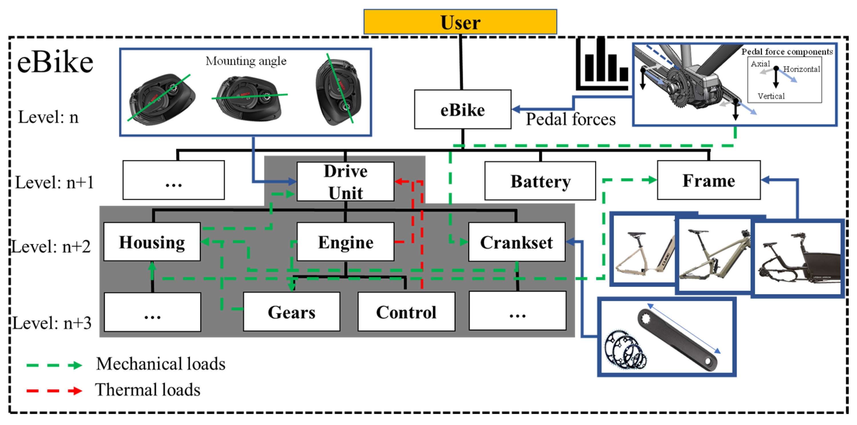
Based on the insights of the previous chapters, it can be stated that the Robust Design of a DU must consider the variance and noise of the load spectrum of both the external and internal DU loads, as well as the different system configurations of the eBike, consisting of its bicycle frame, the crank arrangement and the mounting angle. In Robust Design terminology, the load collective and manufacturing and assembly tolerances represent the noise and aleatory uncertainty and the topology of the housing represents the design parameters. The configurations of the eBike system constitute additional “system parameters”, like the frame or geometry data of the crankset, which must be varied to reduce epistemic uncertainties.
This necessity results in two potential optimization approaches. On the one hand, in order to meet the demand of the bicycle industry to install the DU as a standard component, the optimization of the design parameters can aim at reducing the impact of the noise parameters (or ensuring component safety) for as many system configurations as possible or for all system configurations. On the other hand, this necessity also opens up a new perspective wherein the system parameters can be restricted in order to find an optimal DU for a certain category of system parameters, e.g., based on the bicycle type. In the process, any objective can be selected for optimization, as can be seen in Formulas (2) and (3) below. Typical examples may include minimizing the component weight or dimensions and the product or manufacturing costs. However, as this paper is related to the formation of a probabilistic fatigue constraint, the objective function will not be discussed further. With regard to the targeted fatigue constraint, for each of the two approaches, the existing aleatory uncertainty regarding the diversity of static and rider-dependent dynamic loads must be considered to ensure component reliability.
Using differently sampled load sequences for each load channel, a certain failure probability can be determined across all assessed locations under consideration.
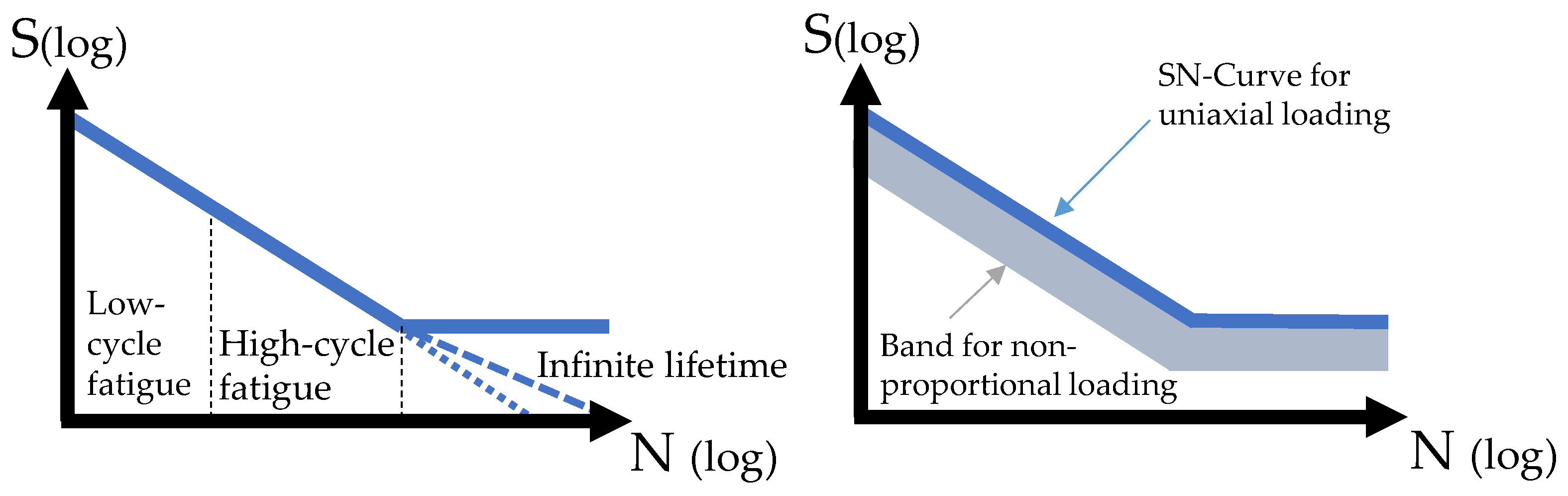
For the eBike DU, the objective is a design in the high-cycle fatigue range of the SN curve similar to the existing norm, which already defines the limit-state function for the fatigue constraint focused on the required service life of the DU. This constraint can be described by a fatigue calculation based on the damage accumulation in a local concept of a selected load sequence and the given design and system parameters. According to Formula (1), a limit for the fatigue constraint corresponding to the accumulated damage can be assumed from a damage sum of 1. The optimization problem can thus be formulated as follows:
minimize :   F ( d A )   or   F ( d A ( s A ) )
subjected   to :     P i ( D a c c ( L A ,   d A , s A ) < 1 f ) < P a l l o w a b l e
with
  • F = objective function describing, e.g., the component weight, manufacturing costs, etc.
  • L A = matrix of sampled load sequences for each load channel according to the desired runtime
  • d A = vector of design variables according to the required application (e.g., bike type)
  • s A , = vector of system variables according to the required application
  • f = scalar-valued safety factor
  • D a c c = damage accumulation
  • P i = vector of the failure probability for the i t h assessed location
  • P a l l o w a b l e = constraint for the tolerated failure probability
To convert this constraint of the service-life requirement into a suitable calculation chain for the evaluation of the limit-state function, the following must be considered with regard to the current state of research (see Section 2) on fatigue calculation:
  • Due to the complex geometry, the use of FEM methods is mandatory to evaluate the limit-state function based on fatigue lifetime.
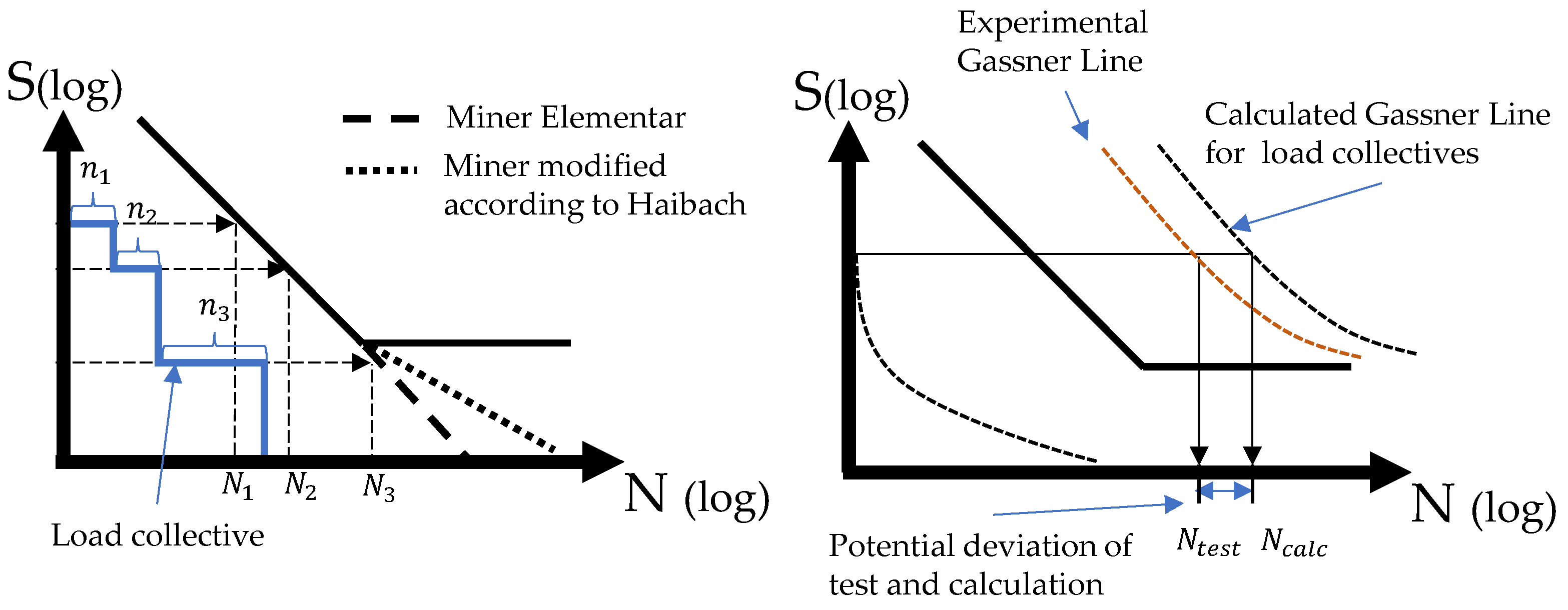
  • The fatigue calculation must be conducted in a cyclic and time-based calculation of realistic load collectives to address the effect of damage accumulation for the fatigue behavior.
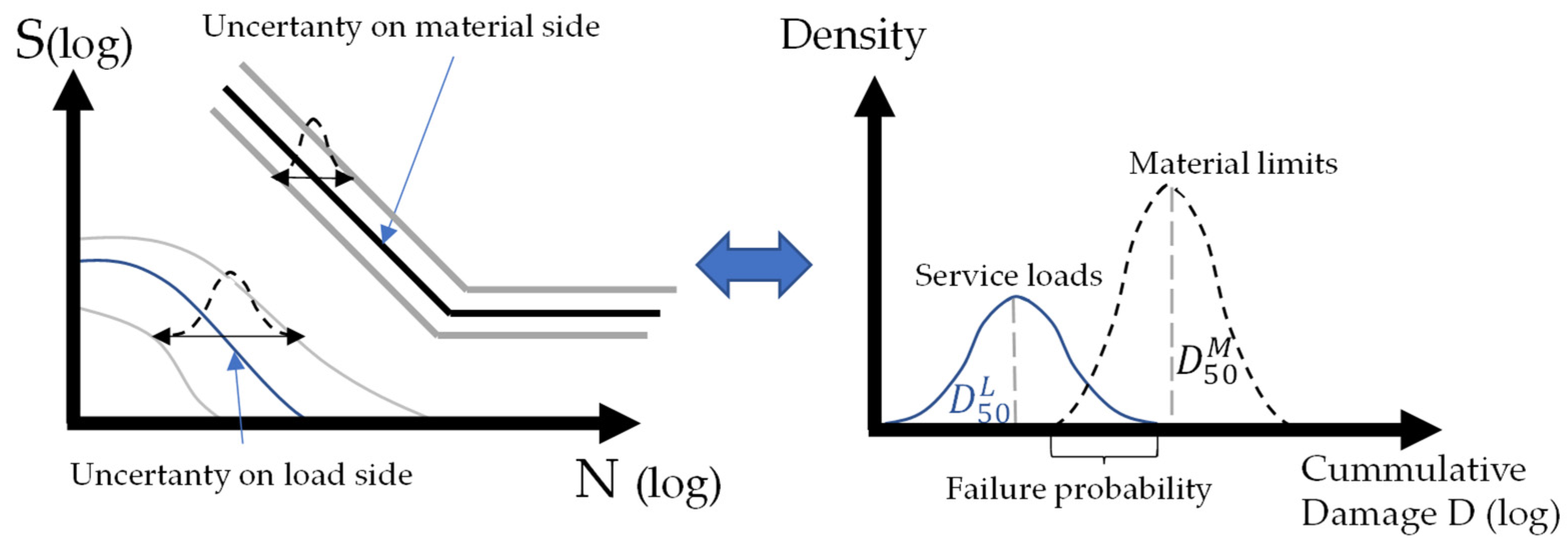
  • The variance of the effective damage in relation to various load-collective compositions associated with different riders and riding situations must be determined to derive the failure probability.
  • The information about the correlation of the different load channels already acquired by measurement can be taken into account in order to characterize the real driving load more precisely.
  • As detailed measurements of the potential loading on the DU are already available, these loads should be considered to form potential load collectives for the fatigue assessment.
  • The multi-axial and simultaneously acting load channels, in combination with different static loads and the complex geometry, imply that a multi-axial and non-proportional load case must be expected at many local areas.
  • A stress-based approach based on the critical planes must be applied with respect to the HCF area in order to perform a suitable fatigue calculation.
  • No general static stress- or strain-based constraints, like those common in examples of RBDO and especially in FORM methods [15,16,56,57], can be applied in service-life calculation. This conclusion arises from the fact that the proper evaluation of reliability must be treated as time-dependent regarding both the calculation of equivalent stress amplitudes for multiaxial non-proportional load cycles and the damage accumulation of potential load collectives.
  • The geometry of the DU housing must be evaluated by multiple local-concept fatigue calculations because no clear critical area and most-likely failure point can be defined prior to the investigation.
Due to the complexity of the eBike DU and the necessity of an accurate fatigue estimation to avoid overly conservative or, worse, unsafe designs, the focus of this paper is on the inner loop of the fatigue calculation. This necessity of a detailed fatigue calculation can be derived from the fact that an uncertainty quantification and a Robust Design approach are not feasible if an unknown error and uncertainty in the fatigue calculation are tolerated by a simplified calculation of the target variable.
Based on the previously defined requirements, a methodical approach for the calculation of fatigue damage based on a simulation and sample-based method, a collective of load time sequences and a critical plane approach can be derived. A sample-based RBDO methodology (see Section 2.2.2) was chosen because of the indisputable necessity of numerical FE simulation, the evaluation of multiple potential failure domains across the geometry and the requirement to evaluate a broadly distributed load collective instead of a single critical load combination. In the process, different load collectives must be formed by sampling techniques regardless of the methodology used.
Instead of the commonly used sampling methods based on statistical variation of individual load-channel amplitudes, samples are taken directly from the measured load sequences, wherein the correlation of each load cycle is already defined. On the one hand, this approach reduces the dimensions to be sampled from many load channels to one cycle, which makes it easier to estimate a representative sample number. On the other hand, unrealistic combinations of load channels and load-time sequences can be avoided, as the already-acquired correlations of the individual load channels are used, not discarded. Additionally, this variation across riders and riding scenarios enables a more explainable evaluation of the fatigue constraint and thus a bicycle-type-oriented design optimization.
To avoid inefficient MC sampling of all the measured load sequences, classifications of the ratio-load channels, the maximum pedal force or torque amplitude can be used to perform space-filling sampling techniques. These classifications can also depend on information about the measured driving situation or the rider, which may yield more interpretable results and the possibility of assessing different riding scenarios.
A probabilistic evaluation can then be obtained by calculating the equivalent stress amplitude for multiple load time sequences of crank cycles from different riding situations, bicycles and riders. In that way, the division into clearly defined sequences of pedal cycles can be seen as a natural separation of the load-time signal, without implementing further cycle-counting procedures. This approach directly enables fatigue calculation for different collectives of these cycles according to the linear damage accumulation.
For this subsequent step, it is crucial to assign the obtained equivalent stress amplitudes to a realistic frequency distribution reflecting the riding behavior. An incorrect frequency assignment will lead to over- or under-dimensioning in the probabilistic evaluation.
This step is decisive, as the main purpose of the existing measurements (Section 3.1) was to predominantly cover higher-loaded sequences. Therefore, finding a reference to realistic frequency values and the probability of occurrence of the more severe load cycles in the field application is highly relevant to generating a realistic fatigue calculation.
This reference value can be obtained from the maximum occurring torque over one pedal cycle, which is recorded by the DU control, thus delivering a representative distribution. Hence, the equivalent stress amplitudes of the sampled and measured crankshaft revolutions can be assigned to their respective frequencies, considering their maximum torques to account for them in a probabilistic fatigue-damage or service-life calculation. The resulting two-dimensional distribution of the potential stress amplitude and its probability of occurrence can further be used for the probabilistic evaluation of the fatigue constraint.
However, for the simulation-based time-based evaluation and calculation of these crank cycles, enormous computing capacities are required. This requirement suggests the need to use surrogate models. In such models, the majority of the computational cost is devoted to the FEM calculation to determine the stress tensor across the time sequence, while a relatively small proportion is required for the calculation of the damage criterion and the critical-planes method.
This use of the surrogate model is supported by the comparatively low computation time of the critical-plane model and the fact that a direct prediction of the surrogate model for the damage of different load cycles and the underlying load time histories for a multi-axial load case is difficult to realize. The reasons for this difficulty lie in the quantity and variety of possible load signals, which are both difficult to parameterize or categorize, and also have far too different properties to allow for training with reasonable effort.
For this reason, the surrogate model should serve as a regressor that can predict or interpolate the local stress-tensor values according to the sampled design, eBike system and load parameters. In this way, the surrogate model delivers the local stress-tensor components of all observed areas of the DU housing for a defined quasi-static load and parameter combination. This approach makes it possible to obtain the sequence of local stress tensors for the fatigue calculation of an arbitrary discretized load-time sequence. The reasons for this approach lie in the quantity and variety of possible load channels, which are both difficult to parameterize or categorize and also have far too many different properties to allow for training with reasonable effort. Thus, by starting with high initial computational effort for the adequate sampling of the selected parameter space and the training and validation of the surrogate model, a regressor can be defined that allows the efficient computation of many load-time sequences due to the extremely low computational effort required for each additional sequence. To further increase the efficiency of the whole approach, the basic but high-fidelity FEM model, as well as the initial parameter space that is used for the calculation of the sample points and the generation of the training data, is subjected to further order reductions. The focus is thus on projective methods that minimize the number of input dimensions in the model. This approach brings the advantages of faster computation time and the ability to compute more sample points to generate a better-performing data-based surrogate model in the same time period. Such a model is crucial if new training data for a new product geometry must be calculated repeatedly in an iterative optimization. On the other hand, this initial dimension reduction generally also increases the efficiency of the data-based surrogate model, as it is (given the same amount of training data) more capable of interpolating between a few dimensions with many expressions than between many dimensions with only one or a few expressions. This difference arises due to the curse of multidimensionality and the exponentially increasing distances between the used samples.
To calculate this fatigue constraint in a local concept across the whole geometry, it is crucial to discretize the complex housing geometry and to evaluate the relevant and critical local areas in separate calculations of the local cumulative damage distribution. This approach is necessary because the enormous diversity of the load spectrum and changes in design and system parameters make it impossible to identify the most critical point in advance of the presented fatigue assessment.
Regarding this discretization, the question naturally arises as to in which steps the geometry must be divided to avoid the disadvantages of a too-large loss of information in an almost global evaluation, as well as the excessive calculation effort required for a very fine grid. Concerning the surrogate-model approach, this discretization offers the possibility of data reduction via a gradient-based clustering procedure to minimize the number of locations for which the surrogate model has to be trained. In summary, the requirements for the computational method consist of computationally efficient simulation and a surrogate model, as well as reasonable discretization and the data structure of the input and output data. In addition, these calculation processes and data evaluations must be implemented with the maximum degree of automation.
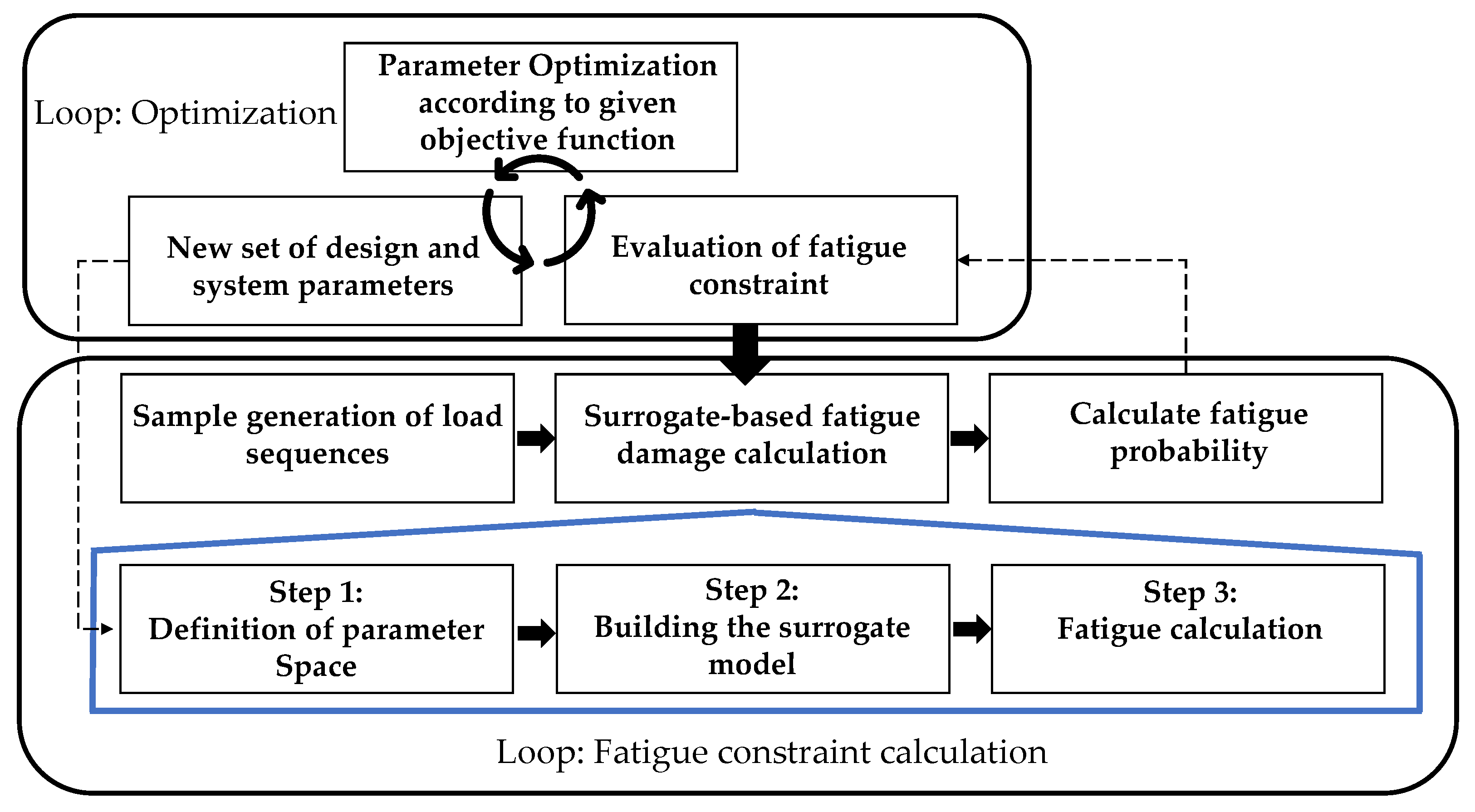
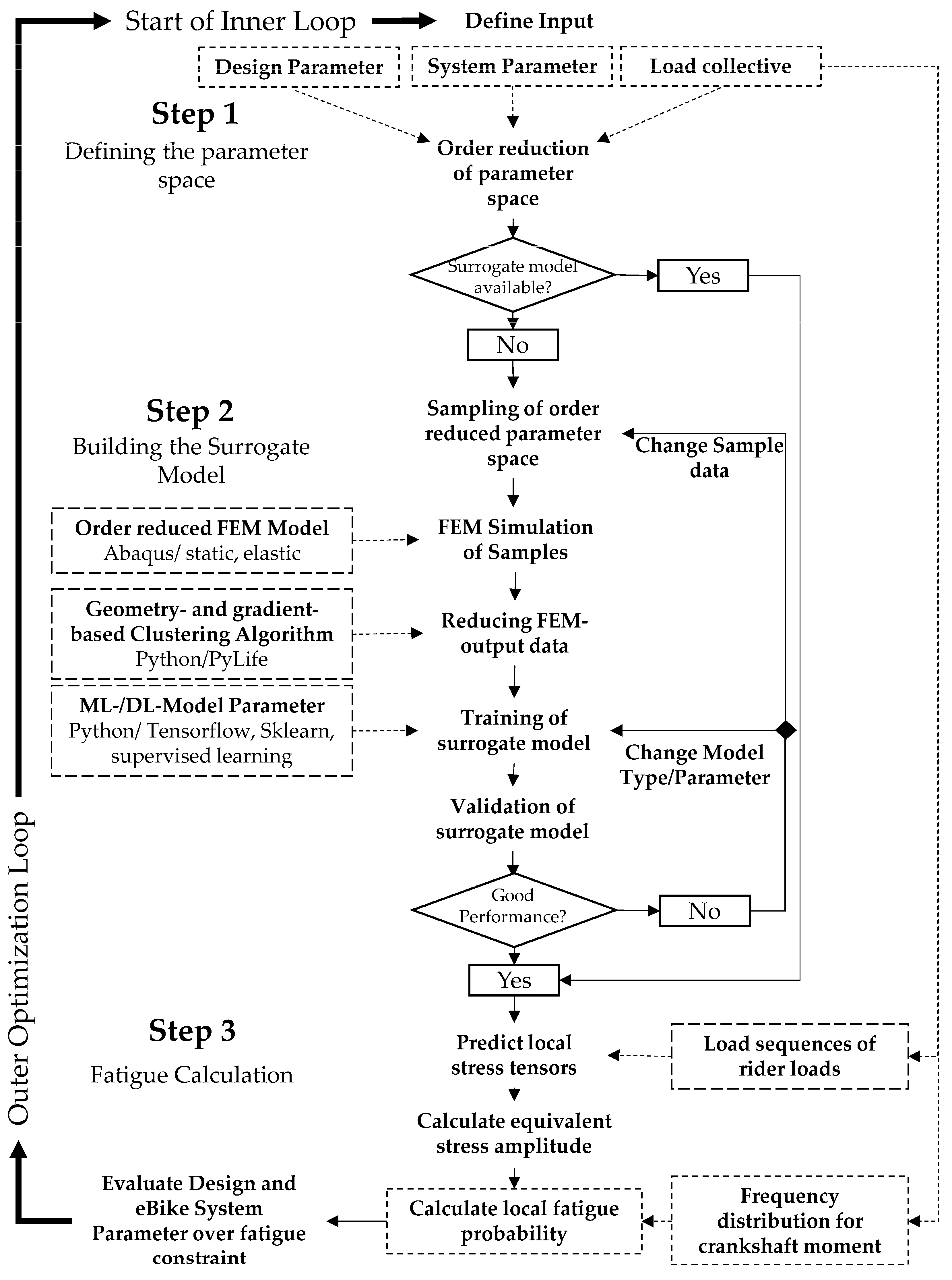
Overall, this necessity leads to a double-looped optimization approach wherein the inner loop calculates the fatigue probability, incorporating the variance in the load collective, and the outer loop is a deterministic parameter optimization of the system and design parameters that can be conducted, e.g., by an evolutionary optimization algorithm and a given objective function. This approach can be seen in Figure 16. A more detailed overview of the proposed procedure and the central topic of the surrogate-based fatigue calculation can be seen in Figure 17. Across the following sections, the individual areas of this methodical procedure and their application to the eBike case study will be addressed in detail.

4.2. Defining the Parameter Space

To avoid the curse of dimensionality and thus the need for an enormously increased amount of sample data, the parameter space for the generation of the training sample and the resulting surrogate model should be reduced as much as possible. To achieve this reduction of the input dimensions within the eBike system, substitute variables were identified inside the DU sub-system that can be described by a mathematical function and the combination of multiple input parameters without the loss of relevant information. To identify these variables, the top-down and bottom-up relationships between the individual components were investigated in a system analysis of the eBike system. The results of this analysis revealed that many relevant influences can be mapped via the stiffness at the frame interface and the resulting bearing load of the DU. With regard to the load and fatigue calculation, further dimension reductions can be achieved by separating the static and dynamic loads. The result is lower-dimension input.
A general overview of the eBike parameters and their dimensional reduction is shown in Figure 18. The applied methods and assumptions are further described below.
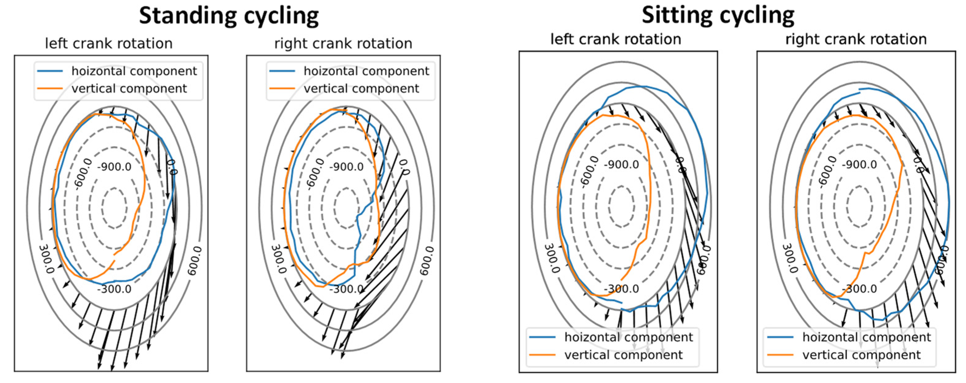
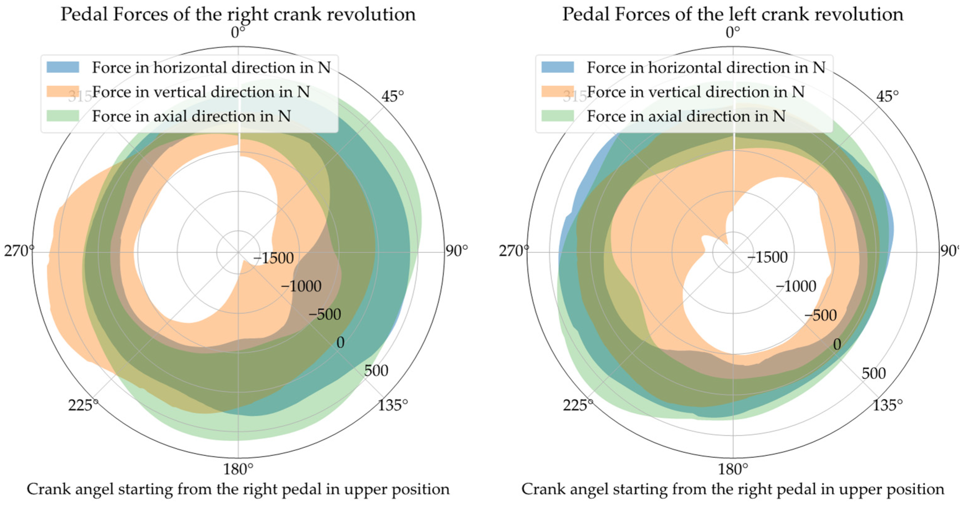
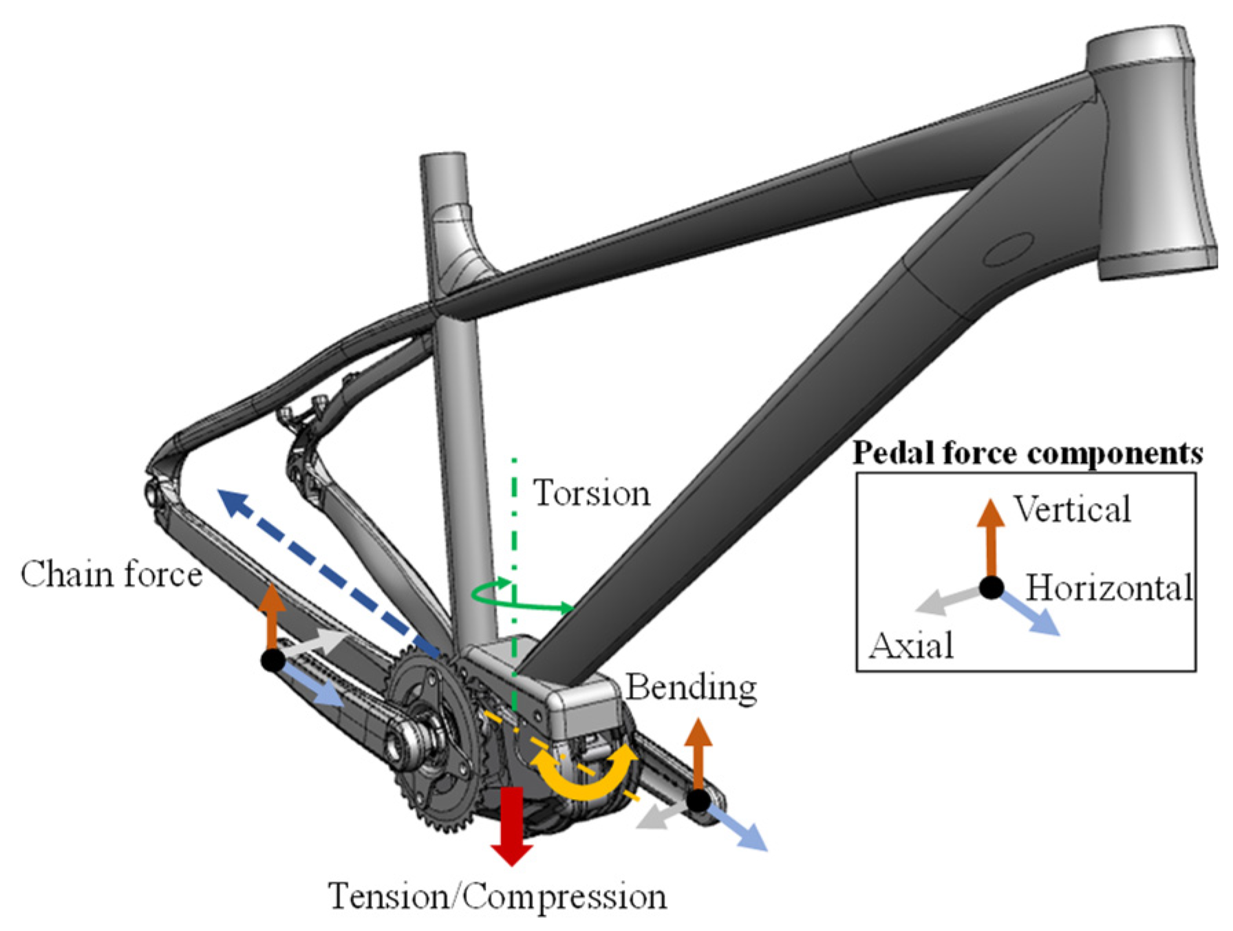
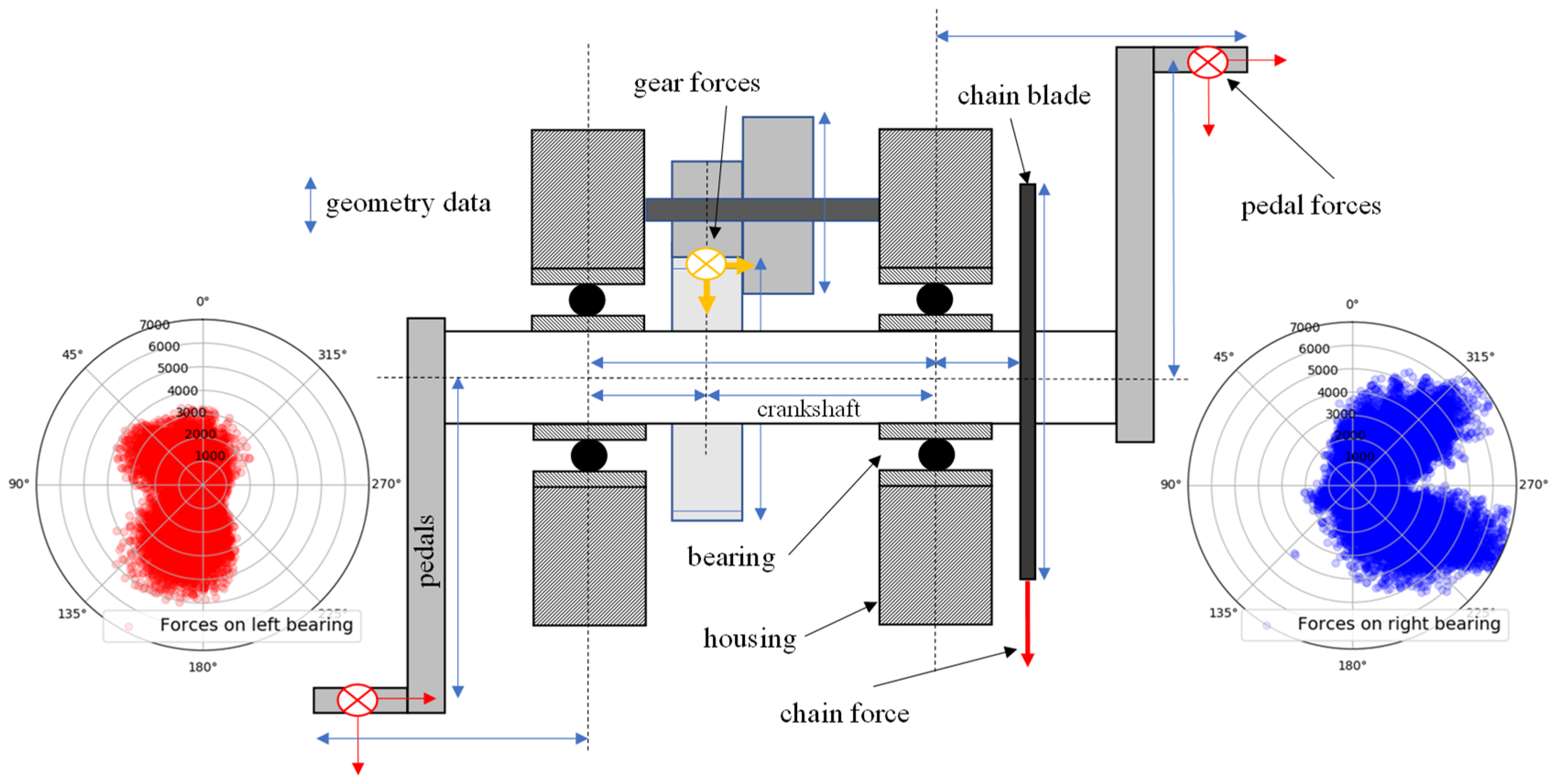
For the dimension reduction of the load channels, the high-resolution load-time sequences of the load-spectrum measurements were superimposed over all relevant geometry parameters of the crank setup and the DU in order to define a resulting radial-bearing load for each measured load situation based on its amplitude and orientation. The assumption was accordingly made that the axial bearing load can be neglected. The reason for this assumption was the low amplitude and relevance of the axial bearing load relative to the radial load. Regarding the overall DU load, the circumferential load resulting from the axial force and the adjusted bearing would be of negligible importance, but would require further input parameters to describe the load condition. Hence, the input dimension of the six pedal-force components, several geometry parameters and the DU engine support could be reduced to the five parameters of amplitude and orientation of the surface pressure in the right and left bearings, as well as the chain force (see Figure 18). These values could be calculated using fundamental mechanical equations. The chain force still must be considered because it introduces a reaction force into the frame via the rear axis. Figure 19, below, illustrates the mechanical forces and the relevant geometries around the crankshaft, as well as the potential range of loads on the right and left bearing. These values can be calculated by superimposing the channels of the measured load collective over all variable geometries of the DU Design. Because the mounting angle of the DU affects only the orientation of the bearing forces due to the rotation of the DU housing around the crankshaft, this system parameter can also be incorporated into the dimension reduction.
Hence, the input variable of the six pedal-force components, several geometry parameters and the DU motor support can be reduced to several correlated values of the five parameters for the amplitude and orientation of the surface pressure in the right and left bearings, as well as the chain force (see Figure 18).
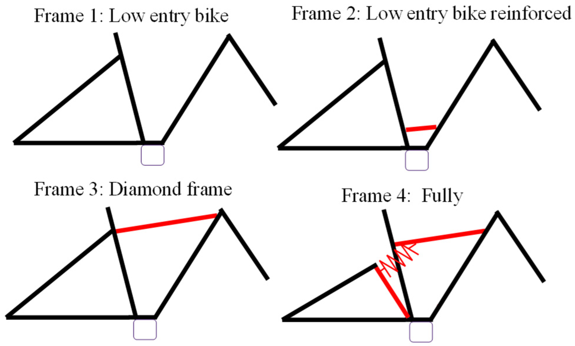
As a simplified description of the connection between the DU and the frame and its boundary conditions, a discrete equivalent-stiffness matrix can be derived for specific bicycle types as an alternative to considering different geometries and materials.
Further reductions can be achieved by the separate consideration of static (thermal and production-related stress conditions) and dynamic loads (depending on the load spectrum of the rider). Thus, the complexity and the size of the DoE can be significantly reduced. This approach is feasible because these two stress states can easily be superimposed in a later step. Obviously, this approach requires the assumption that static and dynamic loads have few to no dependencies and can be calculated separately.
Here it should be mentioned that pretensioning forces that define the contact between the housing parts and the frame interface were also modeled to calculate the dynamic loads in order to ensure a feasible simulation. Following the order reduction of the input parameters and the replacement variables, modifications were also made to the existing and already-validated Abaqus FEM model, which was used for the calculation of the norm requirements. This model consists of the housing, bearing and crank geometry of the DU, which are assembled and pre-tensioned in two initial calculation steps. In a first step, the geometry of the crankshaft and its contact definitions at the DU bearing position were replaced by an analytical description of the surface-pressure profile defined by the orientation, amplitude clearance and geometry of the bearing. This analytical profile was calculated using a Python routine and integrated using a Abaqus subroutine. These routines deliver an easily editable interface for the required automatization of the calculation. Compared to bearing-and-contact modeling, the direct calculation and use of surface pressure is a numerically less error-prone and, above all, more computationally efficient. A comparison with the previously existing FEM model, which had already been validated in detail within the company on the basis of the standard load case, showed no notable differences in results and a significantly minimized computing time.
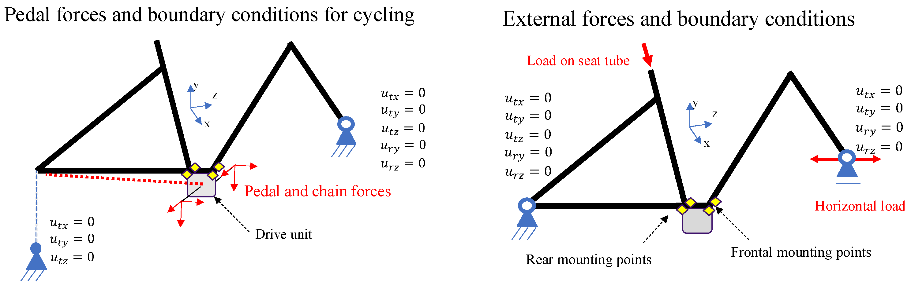
The Frame Interface was added and modeled by the aforementioned equivalent stiffness matrix, which was extracted by the Guyan-Reduction scheme [62]. This scheme represents a projection-based reduced-order modelling technique for the completely meshed bike frame geometry. The Guyan-Reduction condenses the whole stiffness matrix to a linearized stiffness matrix for only a few remaining degrees of freedom. In this case, the remaining degrees of freedom were defined for nodes at the mounting points of the DU, as well as the front and rear axes. The retained nodes were coupled to the rest of the respective geometry by a coupling constraint. Thus, the DU can be mounted and pretensioned at the interface and the boundary conditions can be enforced at the retained nodes of the axis. Further hierarchical simplifications were carried out regarding the material model, which was set to be purely elastic given the targeted fatigue range in the HCF area. Due to the focus on the methodological steps, the already existing FEM model will not be discussed further at this point.

4.3. Building the Surrogate Model

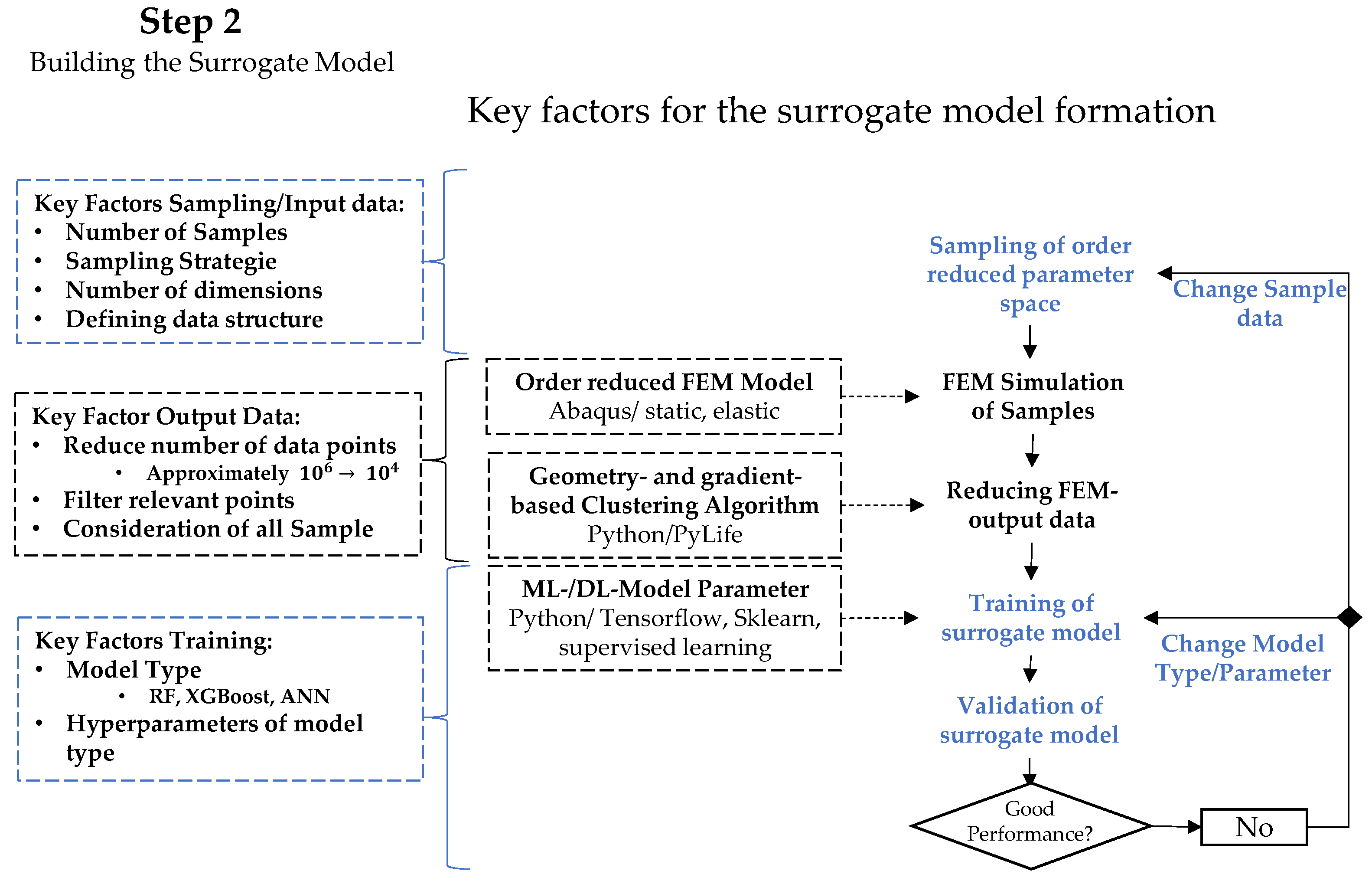
The formation of the surrogate model depends on the two major steps of data generation, including a data reduction to form the output data and the generation of the data-based model. These two steps, as well as their key factors, are highlighted in Figure 16 based on the general methodical approach shown in Figure 20.

4.3.1. Data Generation and Reduction

As an initial step for the creation of the surrogate model, sample data must be created and calculated according to sampled input data and the simulation model. For an adequate representation of the parameter space, the LHS was selected as a space-filling sampling algorithm. To ensure that the FEM simulation model yields sufficient accuracy, a fine discretization and a high element count of more than one million elements must be expected. For this size, data processing and storage, as well as the planned construction of a data-based surrogate model, can be completed only with enormous computational resources.
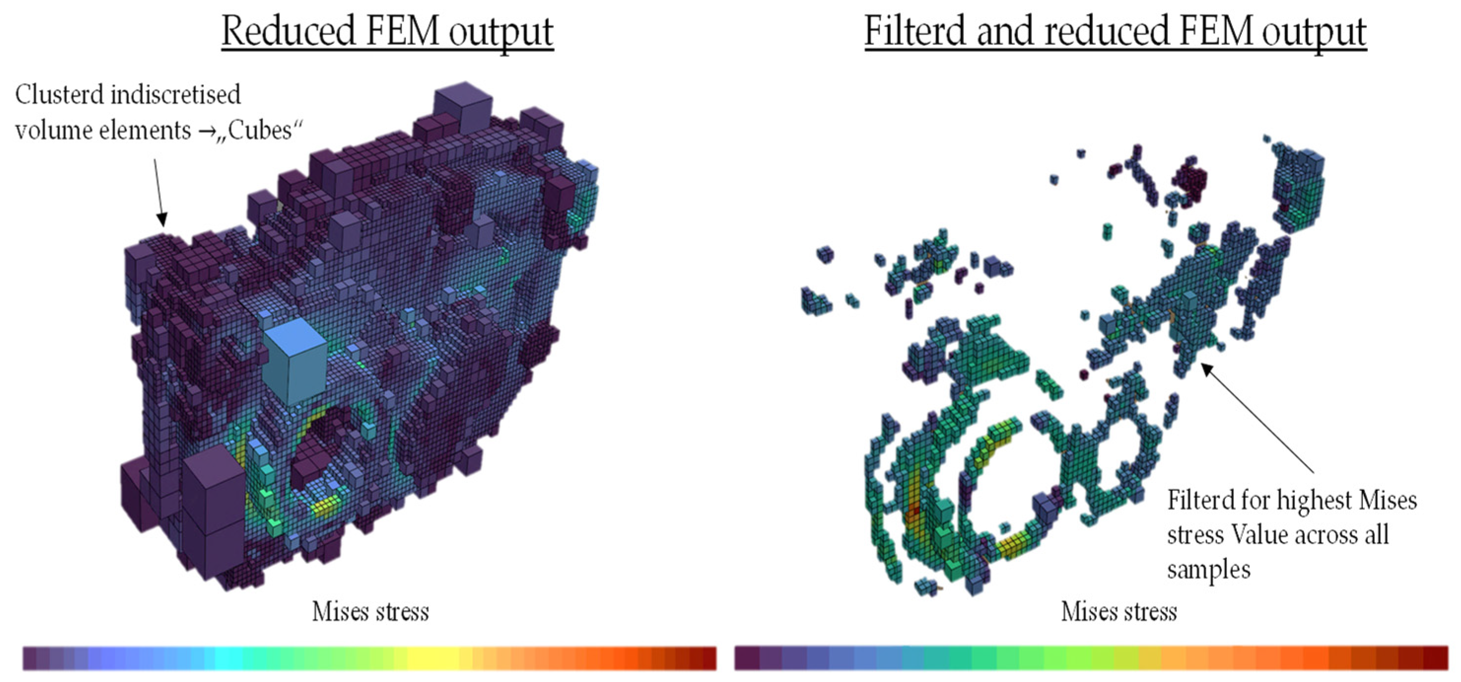
To achieve the required coordinate-based and simultaneously clustered and reduced data structure, a gradient- and volume-based clustering procedure was developed. This method identifies the local maxima of the selected target variable inside an observed volume to build a locally refined but generally coarser mesh via variable discretization. As a convergence condition for this algorithm, suitable threshold values for the gradient and the minimum value, as well as variable and maximum refinement steps of the discretization, are defined. The fundamental idea behind this method is that areas of the FEM mesh that possess nearly constant values over the entire output of the simulated samples can be clustered and described by only one representative value for this volume. Furthermore, areas associated with a very low target value and thus are not relevant to the fatigue calculation can be filtered and excluded.
To generate a clearly defined and coordinate-based discretization pattern of the geometry and the corresponding FEM output, the basic geometry of a cube covering the maximum component dimensions is defined as the starting volume. Subsequently, this initial volume is refined in a manner analogous to the scheme shown in Figure 21, by bisecting the edge lengths of the original cube and its children. The refinement is performed if more than one local maximum of the target value above a certain threshold is detected within an observed volume. This refinement is executed until either a convergence criterion regarding the minimum stress gradient or the minimal cube size is reached.
Finally, this algorithm is intended to provide a significantly reduced discretization with only a slightly reduced information density as a foundation for the training of the data-fit surrogate model. Hereby, of course, it is assumed that the previously simulation-generated sampling data is sufficient to be able to perform this clustering reasonably. However, as the formation of the data-fit surrogate model generally allows only the interpolation of the results, sufficient sampling is inevitable. Therefore, the derivation of the critical points based on the sampled data is seen as a reasonable assumption.
Thus, the relevant parts of the housing can be focused on and represented with a significantly smaller amount of data, leading to an efficient hierarchical order reduction for the database. The distinct algorithm of coordinate-dependent volumes additionally allows the integration of different meshes and simulations. Furthermore, the coordinate-related discretization allows the comparison of different geometries in different optimization loops. Although some cube volumes may be added or omitted due to the geometry change, a large part will remain and can thus contribute to the robust optimization process. Consequently, an application to arbitrary geometries is conceivable.
Each of these cube objects can then be assigned the output values of the target value, its coordinates and the exact parameter definitions of the simulation step, these being the essential information for the data-based surrogate model. Both the algorithm and the required data transfer from the Abaqus output file were programmed in Python. Figure 22, below, shows an example of the reduced discretization of a DU geometry that was simulated for 400 sample points.

4.3.2. Generation of the Data-Based Surrogate Model

For the creation of a surrogate model, the initial task consists of forming the input and output data for supervised learning and selecting an appropriate model type and algorithm. In this case, the input data are built from the load, eBike system and design parameters of the individual samples, which are supplemented on the output side with the evaluated stress-tensor components. The details of the data structure depend on the arrangement and processing of the coordinates-based data of the adapted discretization.
In this way, either individual regression models can be created for each discretized data point, or the adapted and filtered mesh can be considered collectively in one single surrogate model by incorporating the coordinates into the input data to guarantee an unambiguous assignment.
To create individual surrogate models, however, a rapidly increasing memory requirement and high computational costs for the training of the individual models arise for each additional considered location. In light of the filtered yet still respectable number of potentially relevant points (see Figure 19), the following assessment involves only the use of a cumulative data structure within a singular surrogate model, while the approach of several individual surrogate models is ruled out.
However, as this approach is associated with an increase in dimensionality due to the incorporation of the x-, y-, z-coordinates, this increased number of input dimensions is accompanied by a reduction in the sampling quality. The severity of this reduction depends on the number and density of the included data points. In addition to the pure number of incoming sampling points, their geometric distance in the x-, y-, z-coordinates is of particular importance, as this factor has an enormous effect on the spacing of the multidimensional dataset. As can be seen in Figure 21, filtering the data sets to highly loaded locations will lead to an uneven distribution of the sample data. As a result, the training data become increasingly heterogeneous due to the varying influence of geometrically adjacent data points. Therefore, the possible influence of differently finely-distributed data points must be accounted for in model-building and validation.
Besides the data structure, the performance of the surrogate model depends in particular on the model type and its hyperparameters, as well as on the number and selection of the initially calculated training data. To reach a decision in this context, different model types and sample data sets are evaluated by their performance. Due to the iterative application of this fatigue calculation within an optimization loop, the performance is evaluated qualitatively from the ratio of computing time and prediction accuracy.
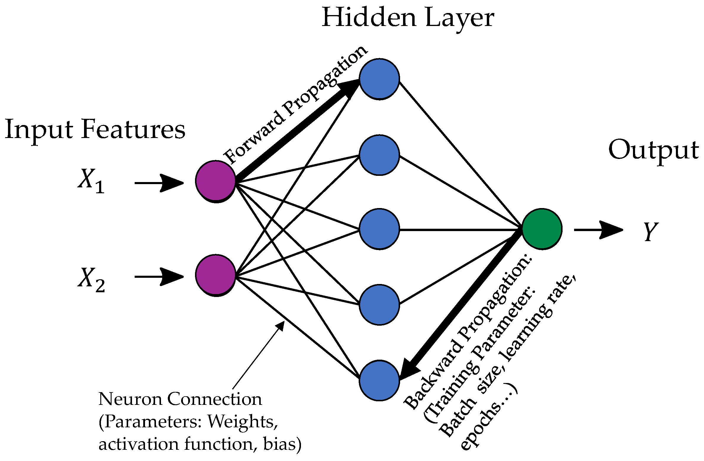
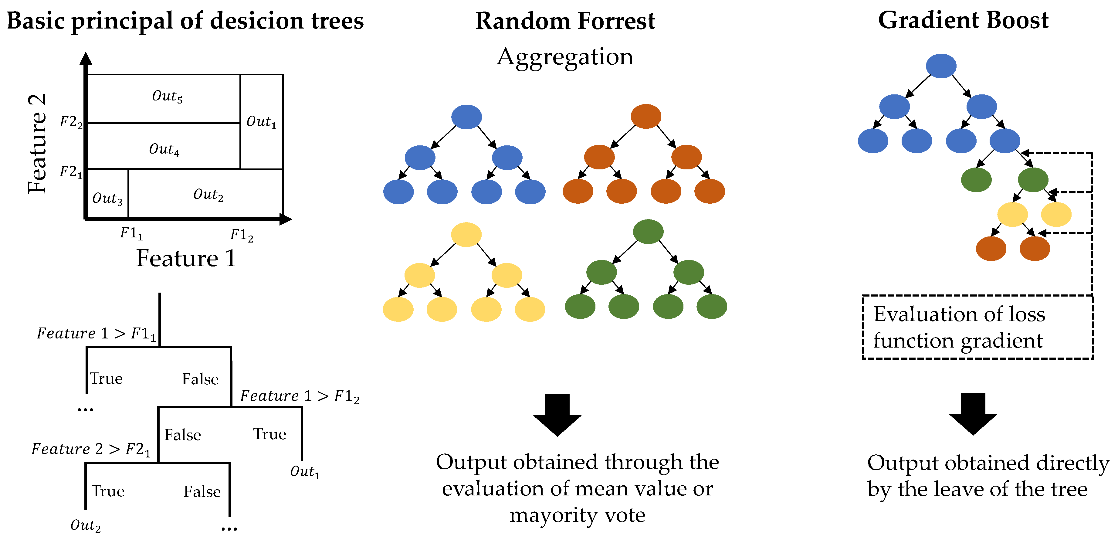
Regarding the algorithm used for building the surrogate model, this study considers supervised learning ML and DL approaches for regression, including tree-based machine learning algorithms in the form of XG and RF, as well as an ANN with multiple hidden layers, to explore this data-driven approach. The selection of these model types was derived from a literature study in which the most common algorithms were evaluated based on fundamental characteristics such as training time, prediction time, precision and their scope of application in terms of the number of features, data size and the number of outputs.
To define a suitable number of training samples, the metrics of the individual model types were evaluated for different sample sizes in steps of 100 FEM samples. This study revealed good model performance for the given input parameter space from a size of 400 sample data sets. The parameter space of this study was set for the entire driver load collective (including different crank-setup geometries), a bicycle frame and an installation position range of 20°. To eliminate the bias arising from different sampling variants, all of these samples were generated by the LHS method.
To evaluate the applicability of the method to different discretization filters and data sizes, the upper 5%, 12.5% and 20% of the data points were selected according to the height Mises equivalent stress across the sample range. Commonly, influences and dependencies from the chosen training and validation dataset were excluded by a ten-fold cross-validation. To evaluate the results, the common metrics of the RMSE and the R 2 value were considered. The RMSE was determined from the mean of all single-tensor component predictions, as well as their combination in the form of the equivalent von Mises stress. To ensure the comparability of the algorithms, an elementary hyperparameter optimization was performed. To keep the computing times for this optimization within a reasonable limit (that would also allow an iterative and practical application of the method), this hyperparameter optimization was carried out only for the lowest amount of data and, in the case of the ANN, only for a limited set of parameters. This approach was based on the assumption that the hyperparameter setting can also be applied to larger data sets without a significant reduction in performance.
The hyperparameter optimization was performed using a Bayesian Optimization algorithm based on the Python module Hyperopt. This optimization was based on minimizing the average RMSE value of the six output channels for the worst-performing data split of the cross-validation by adjusting the hyperparameter settings in a predefined range.
These computations were performed on a PC with a 12 Core CPU of 4,2 GHz and 32 Gb RAM. The data structure was processed using a Python code, and the model types for the ML and DL models were retrieved by the SKlearn and TensorFlow. The results are shown in Table 1.
Based on these results, it can be confirmed that in general, all model types yield good-quality predictions of the results and a sufficient R 2 coefficient. This result is evident regardless of the number of data points considered. However, a general trend of increasing error values can be observed for decreasing numbers of data points. Similarly, the R 2 value decreases for larger sample sizes. This result may be explained by the filtering of the data points according to their quasi-static equivalent stress amplitude, which leads to generally higher absolute values for the collection of filtered data points. Further explanations for this outcome could include the lower dependence on individual mispredictions and the denser quantity of training data for higher numbers of data points.
Nonetheless, it is striking that this trend is significantly weaker for the XG and the ANN than for the RF. Here, the RF shows a generally larger scatter, but also better performance compared to the XG and ANN applications for larger data sets. This result can presumably be explained by the lack of generalization in the XG and ANN model types, which were hyperparameter-optimized only for the smallest data set. In contrast, the RF regressor, which is generally less sensitive to overfitting, shows a more robust performance and the expected trend for a larger and less-filtered data set based on the extreme values. On the other hand, the hyperparameter-optimized XG is the better-performing model for the small data set containing generally higher and more heterogeneous values. Such a result highlights the importance of the hyperparameter optimization. At this point, it may be assumed that the XG also provides the best performance for other sample sizes if a corresponding hyperparameter optimization is used.
Regarding the general model types, lower RMSE values can be seen for the tree-based models of the RF and the XG compared to ANN. This is an important finding, especially because of the significantly longer computing time of the ANN. Thus, the superiority of the tree-based regressors over the ANN for tabular data can be proven based on this data set, in a finding analogous to that of the benchmark study of [42].
For all model types, the expected increase in the RMSE is apparent for the cumulative consideration of the output values based on the Mises stress. In view of the potential stress amplitudes, which amount to 0–200 MPa for this case study, this value also appears to represent a reasonable error. However, the results of the general cross-validation do not allow for a complete validation of the surrogate approach for the time-based assessment of a cyclic load. For this reason, a second validation loop was established to evaluate not only the performance of the surrogate model, but the results of the subsequential fatigue calculation for a series of predicted stress tensors. This validation consisted of a comparison of the results from the fatigue calculation of load sequences calculated by the surrogate model and an FEM simulation.
Therefore, the measurement data from two example crank rotations were discretized into 72 uniform sections of the crank angle and then processed by the FEM model to generate a validation data set for the evaluation of the entire calculation approach. Subsequently, these input data were also processed with the machine learning model of the XG and the RF. The use of the ANN was already excluded due to its poorer performance and the enormous computing time. The results of this second validation loop can be seen in Table 2. For more details of this validation, please refer to [50]. It became apparent that the evaluation of entire load sequences by the critical-planes model, which is fed by the surrogate model, results in even lower error values for the equivalent stress amplitude for this load cycle compared to the mean RMSE of the quasi-static mises equivalent stress of the general cross-validation. Therefore, the principle of a surrogate-based approach for fatigue calculation can be validated.
In addition, the influence of hyperparameter optimization on the two tree-based model types was considered in this second validation loop. For this purpose, both model types were used once with the default settings and once with the optimized hyperparameter settings. The results (Table 2) reveal the robustness of the RF and highlight the necessity and benefit of hyperparameter optimization for the XG.
Overall, it can therefore be concluded that the ANN is not suitable for such high sample sizes and input dimensions due to the enormous computing time it requires. It can be assumed that further performance improvements for the ANN would be possible due to the ability of this model type to learn. Such improvements can be achieved only through investing significantly increased effort in the hyperparameter optimizations, which is simply not cost-effective with the data volumes required for this particular method. The use of the XG regressor is therefore recommended for accurate evaluation. However, hyperparameter optimization is necessary to achieve the necessary generalization and good results. As the computational effort for hyperparameter optimization is rapidly increasing with the number of data points, the sample size should be chosen with respect to the intended objective. For faster estimations that do not focus on low prediction errors, the RF is recommended and can also be used appropriately without hyperparameter optimization. Transferring these findings to the application of this method in different development stages, the RF can be recommended for the concept phase and the rapid testing of different parameter combinations. Conversely, the XG is preferable for more mature designs and especially in the validation phase.

4.4. Fatigue Calculation

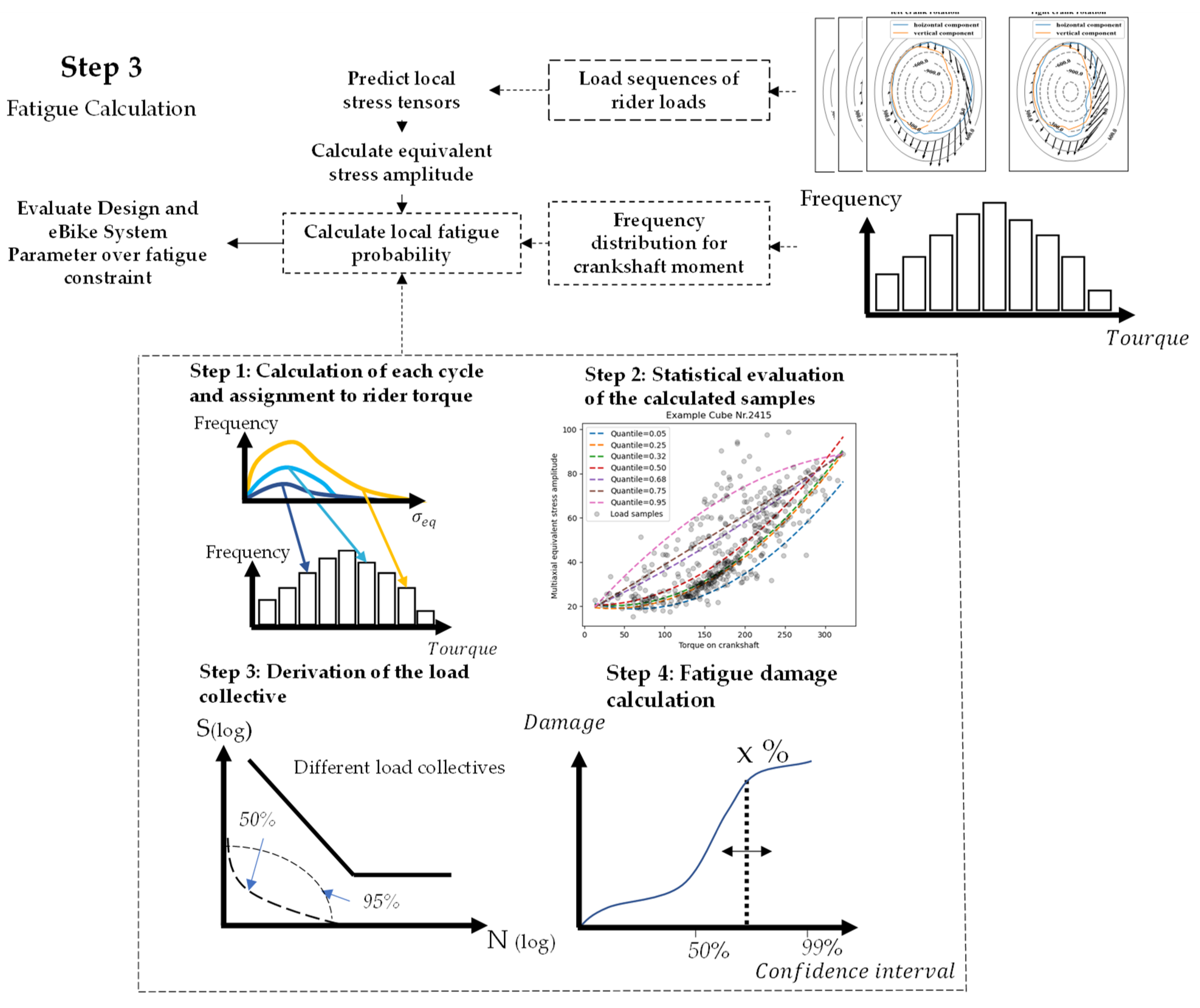
To calculate the service life and the probabilistic fatigue constraint, measured load-time sequences are discretized into a sequence of quasi-static single loads. Subsequently, these loads are combined with the system and DU parameters to generate a sequence of input data for the surrogate model. As a result, the data-based surrogate model provides a sequence of the stress-tensors components for each local area considered during surrogate generation. Based on this sequence, a fatigue calculation incorporating a multiaxial non-proportional damage criterion and based on the critical-plane approach is performed to convert the multiaxial loading sequence to an equivalent cyclic-stress amplitude that can be compared to existing material data from the SN-Curve. The further application of this calculation chain for the formation of a probabilistic fatigue constraint is described in Figure 23 and in the following section.
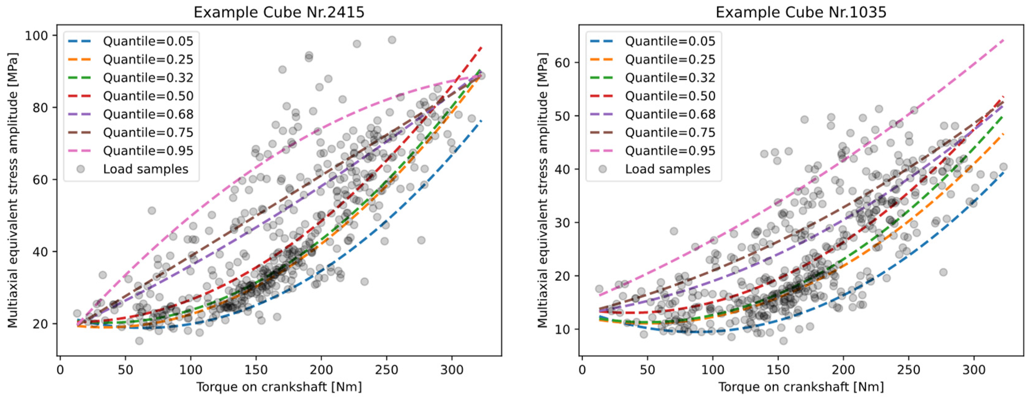
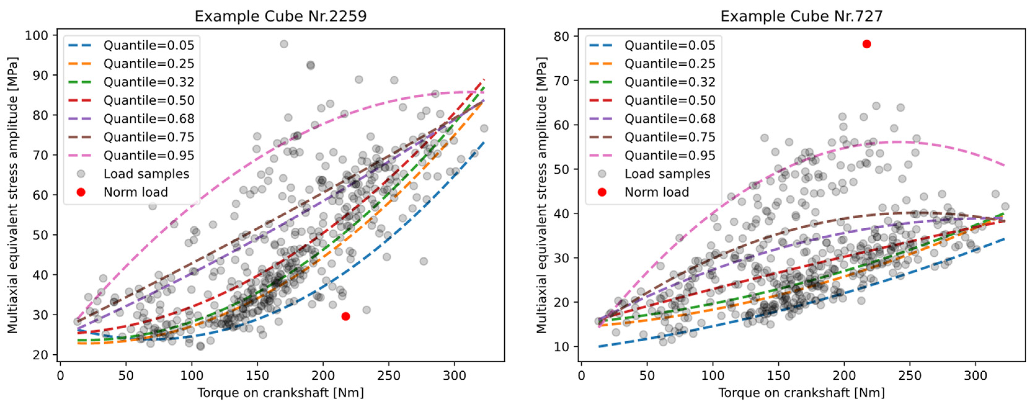
To represent the variance of the driver-load spectrum, multiple load sequences were sampled from the measurement data and evaluated for one configuration of the DU and the bicycle system. To obtain a reference value for the likelihood of occurrence of each load sequence, the maximum torque (where the distribution is known from the DU recording) on the crankshaft was captured for each sequence.
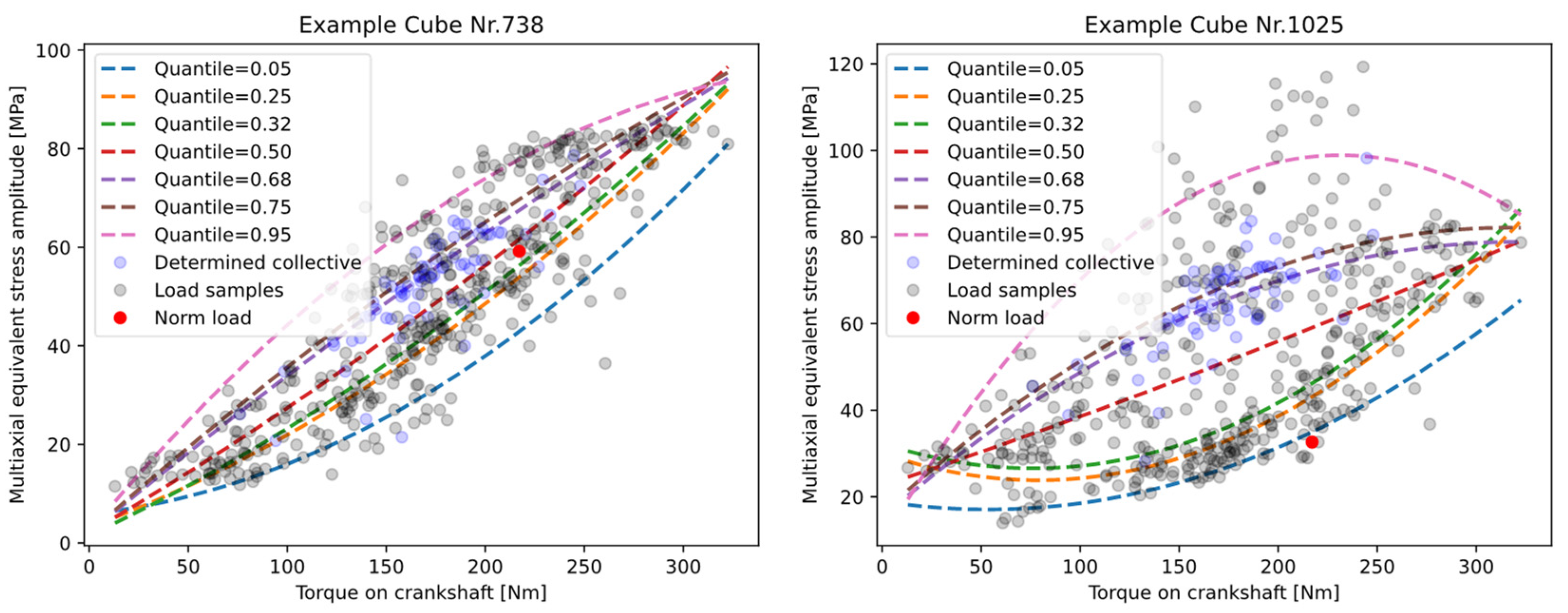
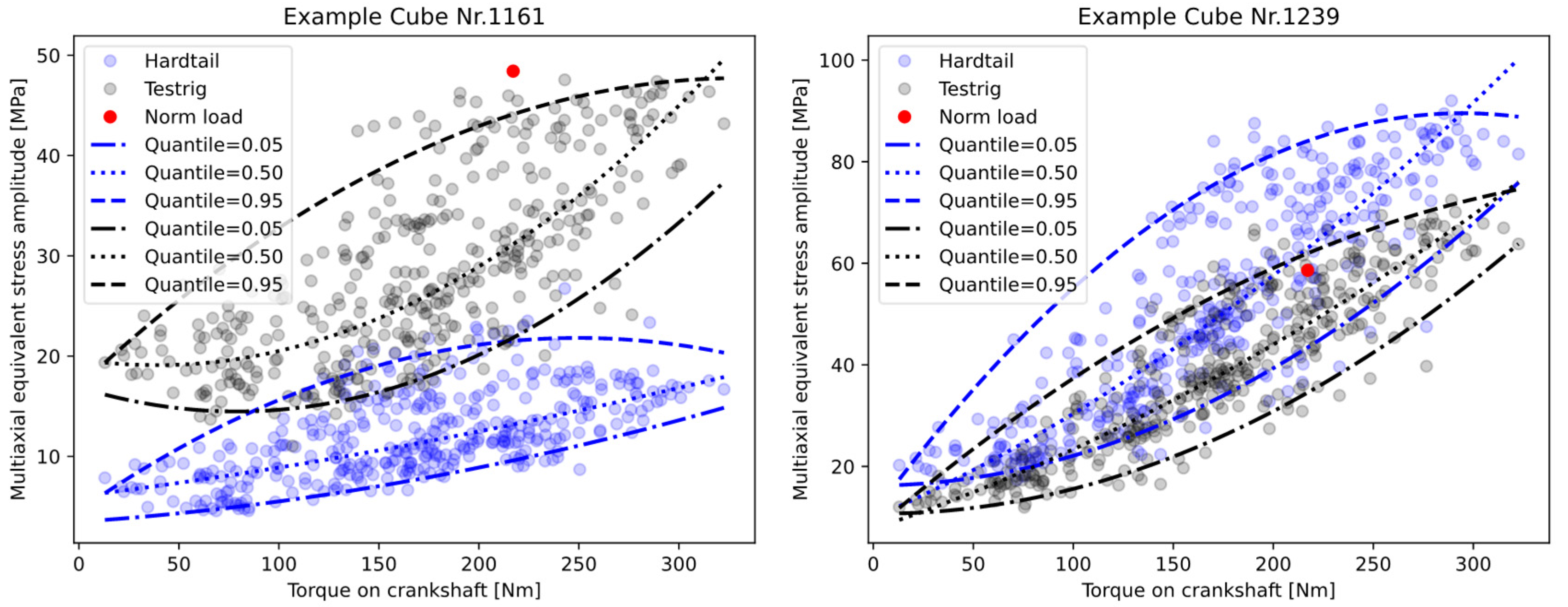
Subsequently, all the equivalent stress amplitudes of the selected load sequences wee assigned to their maximum torque. To evaluate this sample of a discrete 2D distribution, a regression fit based on the quantiles of this assignment was performed to evaluate and represent the variance. Thus, a system of functional descriptions was formed. This system extrapolates the statistical sample distribution to a continuously described distribution of equivalent stress amplitudes over the maximum acting crankshaft torque. Dependent on the order of the function type used for the regression, non-Gaussian distributions can also be determined along the driver torque. In the next step, these functions can be used to determine the load collective for an arbitrary confidence interval and a given torque distribution. This information can then be used to estimate the fatigue life for a given operating time or driving distance, which again can be converted to an effective damage value via the linear damage accumulation and the material data from the SN- curve. As this evaluation can be conducted for several confidence intervals, this information can be transferred to a probabilistic service-life constraint. Figure 24 illustrates this evaluation based on the evaluation of the quantile regression fits for selected local areas of the housing. The function type for the regression was quadratic and according to Formula (4), with m , a and t as the variables for the regression fit, can be represented as follows:
y = m x + a x 2 + t
Furthermore, this evaluation can provide vital information about the robustness of the evaluated local area of the housing to the potential load collectives. From the mean value and standard deviation of the accumulated damage over a given torque distribution and frequency, scalar values for the evaluation of the respective design and system parameter combinations can be determined. This evaluation of the damage must be performed based on the regression functions of a specified confidence interval or quantile, as a normal distribution cannot be assumed for this two-dimensional distribution. As an example, the damage evaluation of the 50% and 95% quantile can be conducted to derive the mean value and the variance. Next, the quantile functions can be used to calculate a load collective based on a required service life and torque distribution to obtain the load collective and the damage value according to the linear damage accumulation. Besides the binary information of failure or no failure for the fatigue constraint, this probability-based information can deliver key information for the evaluation and optimization of the robustness of the DU.

5. Results and Application

In addition to the potential application of this method to parameter optimization, the detailed damage calculation has been used for the evaluation of the normative load case, in contrast to the variance of the measured load collective. For this purpose, the equivalent stress amplitude of the norm load case, consisting of the left and right purely vertical pedal load, was added to the torque and equivalent stress distribution of 500 sample sequences of the load collective. To ensure that this investigation is comparable, no bicycle frame was considered and the test rig of the normative testing requirement was used for all load sequences. The results revealed many local areas of the housing where the loads of the norm load case do not cause critical equivalent stress amplitudes, while the variance of the load collective reveals significantly higher loads with more or less scattering of the distribution. Apart from a few exceptions, the results usually showed a less conservative loading of the normative load case, which was mostly within the scatter band or in its lesser-loaded areas. For the exceptions, however, the standard load case also revealed local areas with a higher stress amplitude than the scatter band of the real load spectra.
Examples of this evaluation are shown in Figure 25. It can thus be shown that the standard test, which is designed for a single worst-case load, shows an overspecification that can restrict the design and further optimizations. On the other hand, the norm proves to be non-conservative and not robust at several local spots when compared to real field loads of lower amplitude but different orientations. This finding is crucial in terms of component safety.
However, this result clearly shows that the cyclic but one-dimensional norm load case should not be applied as the only release criterion for a robust and safe design of an eBike DU.
As these results could be determined on two different DU housing geometries of different series and as the test requirements had already been questioned after the measurement of the load collectives and the literature review, it can be assumed that this observation can be transferred to the DU design generally.
A consideration of the complexity of the housing geometry reveals that multiple multi-axis load sequences result in a large spread for the equivalent stress amplitudes for individual local notches of the geometry. Obviously, this variance cannot be accommodated by a superposition of a single uniaxial alternating load case and its constant chain force. The discrepancy can be explained by the different load combinations caused by the inclusion of all Cartesian pedal-force components and a total crank rotation in contrast to a cyclic load at a constant crank angle. This discrepancy may not be as significant for the original norm application for the almost rotationally symmetrical crankshaft or bearing of conventional bicycles because the load conditions here are caused by cyclic bending and torsional loading independent of the pedal orientation. However, for eBike Dus, it is therefore recommended to avoid designing or optimizing and thus specializing the design based only on the norm load case; that case can be applied only to a limited extent to the non-rotationally symmetrical geometry of the DU housing and its boundary conditions.
In addition to the evaluation of the norm load, the results up to a specified and local threshold value show the expected correlation between higher equivalent stress amplitudes and increasing operating torque. This trend is more or less pronounced depending on the local point, a variation that is presumably attributable to the sensitivity of the individual points to either the chain force and the drive load or the pedal loads. However, different degrees of scattering of the equivalent stress amplitude across the torque range can be observed. Such variation across different riders and riding situations clearly shows the importance of considering a Robust Design approach to design a reliable eBike drive train. These results should therefore encourage the further development or extension of the existing normative requirements to provide the growing eBike market with a robust and safe product design.
To define an alternative load collective capable of extending the current normative load case, load sequences were sought that cause above-average cumulative damage across most of the locally assessed points of the geometry. Thus, a compact load-time series of multi-axis load channels should be defined to represent the range of driver loads for a robust and conservative design. This definition was approached using a straightforward optimization loop that determines the load cycle composition according to a desired damage level and incorporates a penalty for deviations from the desired damage or equivalent stress level for all considered local areas. An example of such an alternative load collective can be seen in Figure 26.
Apart from the pure evaluation of the load collectives with regard to service life, this method also opens the possibility of assessing other influences, like the static loads from assembly processes, thermal expansion or different frame types over the variation of the driver load collective. As an example, Figure 27 shows the effect of a bike frame for potential driver loads and at two chosen data points of the geometry. This result clearly demonstrates that the integration of a bicycle frame results in significant differences in loading. As in the evaluation of the load spectrum, it can be observed that the frame may result in both conservative and less-conservative loads. The modified boundary condition and the stiffness of the DU interface also show a clear influence on the dispersion of the cyclic load amplitude. Similarly, an over- or under-dimensioning is also possible due to a the disregard of the frame. In general, this result confirms the influence of the frame assumed by the preliminary investigation in [6]. Considering the results of these investigations, it can also be anticipated that testing of other frame types will result in further deviations in the results of a systematic test of the eBike compared to a pure component test. Thus, the bicycle frame should be included in any reliable assessment of the eBike as a complete system.
Comparable studies can be carried out for any other superpositions with system and design variables, as well as thermal- or manufacturing-related static load cases for each local discretized volume of the geometry. Based on the results, further methods such as a sensitivity analysis can be performed to gain information about critical loads and parameters for design. Due to the probabilistic evaluation, a suitable confidence interval can always be selected. The method thus proves to be a valuable and versatile analysis tool for robust optimization, as well as for the investigation of a system.

6. Conclusions

Overall, this paper presents the methodological procedure for Robust Design and uncertainty quantification, in which the variance of user- and riding situation-dependent load collectives for a reliability-based optimization can be considered using a probabilistic fatigue constraint regarding the service life. From a methodological point of view, the decisive factors here are the application to a real and complex geometry of the eBike DU and the detailed time- and cycle-dependent calculation of different samples of the multi-axis non-proportional loads to obtain a probabilistic fatigue constraint. The enormous computational effort, which is generally seen as the biggest constraint in both time-based fatigue calculations and the application of RBDO methods for industrial problems, could be reduced to a reasonable scale by combining suitable data- and order-reduction methods.
The key factors to achieving this result (compared to the common computational limitations) were the implementation of a decision tree-based surrogate model for the prediction of the stress tensor and the data—reduced discretization that was derived from quasi-static equivalent stresses of the training samples. Together, these changes enable the examination of the entire geometry with significantly less computational effort. For the selection and validation of this surrogate model type, common cross-validations and hyperparameter-oriented model types were applied. This analysis was conducted to determine the required sample size for the initial training and to validate the surrogate approach for the fatigue calculation. The results showed the superiority of tree-based regressor models considering computation time and robustness, as well as performance, which was determined based on the loss function. This finding is in accordance with existing benchmarks for large amounts of heterogenous tabular data.
The secondary validation loop, in which the desired fatigue calculation was performed using the surrogate model and two FEM-simulated load sequences, validated the application of the surrogate prediction to the fatigue calculation and showed no major mismatches due to the effect of a summed error of the individual tensor component predictions. Thus, the application of this method to the probabilistic consideration of variable load collectives in a time-based fatigue calculation can be verified. Based on the results and the typical requirements of a product-development cycle, recommendations could be made for the use of the robust and rapidly trained RF for the early development phases, with the potentially more accurate but more computationally intensive XG reserved for the later development phases, wherein its potentially higher accuracy is more important. The implementation of a hyperparameter optimization for the XG seemed to increase the performance.
From a product-development point of view, it should be emphasized that the use of real load collectives provides a huge advantage in terms of the interpretability of the results. As a result, certain use cases can be evaluated and used for optimization. In addition, this finding opens the possibility of using a sensitivity analysis to identify the critical factors and loading situations.
With regard to the case study, the eBike DU, the influencing factors that were initially identified in individual investigations were also investigated in a holistic analysis using the proposed method. Overall, these investigations showed relevant differences in the complex and real loading situation in comparison to the existing normative requirements. Therefore, an extension of the norm requirements is recommended. In addition to considering different pedal and chain forces, real-world boundary conditions and frame stiffnesses should also be considered in constructing systematic eBike requirements. Obviously, this approach would result in a more complex testing procedure for the bicycle industry. However, in light of the rapid development and electrification of the bicycle industry, such a change is probably indispensable to ensure product safety and the progress of the industry.

Author Contributions

Conceptualization, M.S. and S.H.; methodology, M.S.; software, M.S.; validation, M.S.; formal analysis, M.S.; investigation, M.S.; data curation, M.S.; writing—original draft preparation, M.S.; writing—review and editing, S.H.; visualization, M.S.; supervision, S.H. All authors have read and agreed to the published version of the manuscript.

Funding

This research received no external funding.

Data Availability Statement

Data available on request due to restrictions e.g., privacy or ethical. The data presented in this study are available on request from the corresponding author. The data are not publicly available due to Company related data.

Acknowledgments

This work would not have been possible without the financial support and the provided resources of Robert Bosch GmbH.

Conflicts of Interest

Author M.S. was employed by the company Robert Bosch GmbH. Author S.H. declares that the research was conducted in the absence of any financial relationships that could be construed as a potential conflict of interest.

References

  1. Bosch eBike Systems. Performance Line SX. Available online: https://www.bosch-ebike.com/de/produkte/performance-line-sx (accessed on 30 June 2023).
  2. Steck, M.; Husung, S. SYSTEMATIC OPTIMISATION PROCESS FOR AN EBIKE DRIVE UNIT IN A HIGHLY VARIABLE ENVIRONMENT. Proc. Des. Soc. 2023, 3, 3305–3314. [Google Scholar] [CrossRef]
  3. DIN EN ISO 4210-8; Cycles—Safety Requirements for Bicycles—Part 8: Pedal and Drive System Test Methods. Beuth Standards Solutions: Berlin, Germany, 2014.
  4. DIN EN 15194; Cycles—Electrically Power Assisted Cycles—EPAC Bicycles—E-PAC. Beuth Standards Solutions: Berlin, Germany, 2017.
  5. Steck, M.; Husung, S.; Hassler, J. Determination and systematization of load situations for eBike drive units as basis for their design and optimization. In Proceedings of the 8th IFToMM-D-A-CH Konferenz, Online, 24–25 February 2022. [Google Scholar] [CrossRef]
  6. Steck, M.; Husung, S.; Hassler, J. Determination and characterization of the influences of the bike frame on eBike drive units as the basis for their design and optimization. In Proceedings of the 9th IFToMM-D-A-CH Konferenz, Basel, Switzerland, 16–17 March 2023. [Google Scholar] [CrossRef]
  7. Soden, P.D.; Adeyefa, B.A. Forces Applied to a Bicycle during normal Cycling. J. Biomech. 1979, 12, 527–541. [Google Scholar] [CrossRef] [PubMed]
  8. Davis, R.; Hull, M. Measurement of pedal loading in bicycling: II. Analysis and results. J. Biomech. 1981, 14, 857–872. [Google Scholar] [CrossRef] [PubMed]
  9. Mimmi, G.; Rottenbacher, C.; Bonandrini, G. Pedalling Strength Analysis in Pathological and Non-pathological Subjects on Cycle-ergometer Instrumented with Three-components Pedals. In Proceedings of the 12th IFToMM World Congress, Besançon, France, 17–21 June 2007. [Google Scholar]
  10. Jurecka, F. Robust Design Optimization Based on Metamodeling Techniques; Schriftenreihe des Lehrstuhls für Statik TU München; Shaker Verlag: Aachen, Germany, 2007; ISBN 9783832263904. [Google Scholar]
  11. Taguchi, G.; Chowdhury, S.; Wu, Y. Taguchi’s Quality Engineering Handbook; John Wiley & Sons Inc.: Hoboken, NJ, USA, 2005. [Google Scholar]
  12. Eifler, T.; Campean, F.; Husung, S.; Schleich, B. Perspectives on Robust Design—An Overview of Challenges and Research Areas across Industry Fields. Proc. Des. Soc. 2023, 3, 2885–2894. [Google Scholar] [CrossRef]
  13. Welzbacher, P.; Puchtler, S.; Geipl, A.; Kirchner, E. Uncertainty Analysis of a Calculation Model for Electric Bearing Impedance. Proc. Des. Soc. 2022, 2, 653–662. [Google Scholar] [CrossRef]
  14. Campean, F.; Delaux, D.; Sharma, S.; Bridges, J. Reliability research roadmapping workshop: Implications for engineering design. Proc. Des. Soc. Design Conf. 2020, 1, 2465–2474. [Google Scholar] [CrossRef]
  15. Lopez, R.; Beck, A. Reliability-Based Design Optimization Strategies Based on FORM: A Review. J. Braz. Soc. Mech. Sci. Eng. 2012, 34, 506–514. [Google Scholar] [CrossRef]
  16. Haupin, R.J.; Hou, G.J.-W. A Unit-Load Approach for Reliability-Based Design Optimization of Linear Structures under Random Loads and Boundary Conditions. Designs 2023, 7, 96. [Google Scholar] [CrossRef]
  17. Chao, H.; Byeng, D.Y.; Wang, P. Engineering Design under Uncertainty and Health Prognostics; Springer Series in Reliability Engineering; Springer: Cham, Switzerland, 2019. [Google Scholar] [CrossRef]
  18. Shittu, A.A.; Kolios, A.; Mehmanparast, A. A Systematic Review of Structural Reliability Methods for Deformation and Fatigue Analysis of Offshore Jacket Structures. Metals 2020, 11, 50. [Google Scholar] [CrossRef]
  19. Chun, J. Reliability-Based Design Optimization of Structures Using the Second-Order Reliability Method and Complex-Step Derivative Approximation. Appl. Sci. 2021, 11, 5312. [Google Scholar] [CrossRef]
  20. Ni, P.; Li, J.; Hao, H.; Yan, W.; Du, X.; Zhou, H. Reliability analysis and design optimization of nonlinear structures. Reliab. Eng. Syst. Saf. 2020, 198, 106860. [Google Scholar] [CrossRef]
  21. Dudzik, A. Reliability Assessment of Steel-Aluminium Lattice Tower. IOP Conf. Ser. Mater. Sci. Eng. 2017, 245, 032072. [Google Scholar] [CrossRef]
  22. Tabandeh, A.; Jia, G.; Gardoni, P. A review and assessment of importance sampling methods for reliability analysis. Struct. Saf. 2022, 97, 102216. [Google Scholar] [CrossRef]
  23. Gong, C.; Dan, M.F. An efficient time-dependent reliability method. Struct. Saf. 2019, 81, 102216. [Google Scholar] [CrossRef]
  24. Hu, Y.; Lu, Z.; Jiang, X.; Wei, N.; Zhou, C. Time-dependent structural system reliability analysis model and its efficiency solution. Reliab. Eng. Syst. Saf. 2021, 216, 108029. [Google Scholar] [CrossRef]
  25. Simpson, T.W.; Peplinski, J.D.; Koch, P.N.; Allen, J.K. Metamodels for computer-based engineering design: Survey and recommendations. Eng. Comput. 2001, 17, 129–150. [Google Scholar] [CrossRef]
  26. Wang, G.G.; Shan, S. Review of metamodeling techniques in support of engineering design optimization. J. Mech. Des. 2007, 129, 370–380. [Google Scholar] [CrossRef]
  27. Eldred, M.; Dunlavy, D. Formulations for Surrogate-Based Optimization with Data Fit Multifidelity and Reduced-Order Models. In Proceedings of the 11th AIAA/ISSMO Multidisciplinary Analysis and Optimization Conference, Portsmouth, VA, USA, 6–8 September 2006. [Google Scholar] [CrossRef]
  28. Kudela, J.; Matousek, R. Recent advances and applications of surrogate models for finite element method computations: A review. Soft Comput. 2022, 26, 13709–13733. [Google Scholar] [CrossRef]
  29. Sudret, B.; Marelli, S.; Wiart, J. Surrogate models for uncertainty quantification: An overview. In Proceedings of the 11th European Conference on Antennas and Propagation, Paris, France, 19–24 March 2017; pp. 793–797. [Google Scholar] [CrossRef]
  30. Koeppe, A. Deep Learning in the Finite Element Method. Ph.D. Thesis, Rheinisch-Westfälische Technische Hochschule Aachen University, Aachen, Germany, 2021. [Google Scholar] [CrossRef]
  31. Hoffer, J.G.; Geiger, B.C.; Ofner, P.; Kern, R. Mesh-Free Surrogate Models for Structural Mechanic FEM Simulation: A Comparative Study of Approaches. Appl. Sci. 2021, 11, 9411. [Google Scholar] [CrossRef]
  32. Greve, L.; van de Weg, B.P. Surrogate modeling of parametrized finite element simulations with varying mesh topology using recurrent neural networks. Array 2022, 14, 100137. [Google Scholar] [CrossRef]
  33. Kohar, C.P.; Greve, L.; Eller, T.K.; Connolly, D.S.; Inal, K. A machine learning framework for accelerating the design process using CAE simulations: An application to finite element analysis in structural crashworthiness. Comput. Methods Appl. Mech. Eng. 2021, 385, 114008. [Google Scholar] [CrossRef]
  34. Shan, S.; Wang, G.G. Survey of modelling and optimization strategies to solve high-dimensional design problems with computationally-expensive black-box functions. Struct. Multidisc. Optim. 2010, 41, 219–241. [Google Scholar] [CrossRef]
  35. Shina, S. Industrial Design of Experiments—A Case Study Approach for Design and Process Optimization; Springer: Cham, Switzerland, 2022. [Google Scholar] [CrossRef]
  36. Nelles, O. Nonlinear System Identification—From Classical Approaches to Neural Networks, Fuzzy Models, and Gaussian Processes; Springer: Cham, Switzerland, 2020. [Google Scholar] [CrossRef]
  37. Hastie, T.; Tibshirani, R.; Friedman, J. The Elements of Statistical Learning—Data Mining, Inference, and Prediction, 2nd ed.; Springer Series in Statistics; Springer: New York, NY, USA, 2009. [Google Scholar] [CrossRef]
  38. Singh, A.; Thakur, N.; Sharma, A. A review of supervised machine learning algorithms. In Proceedings of the 3rd International Conference on Computing for Sustainable Global Development (INDIACom), New Delhi, India, 16–18 March 2016. [Google Scholar]
  39. Yao, S.; Kronenburg, A.; Shamooni, A.; Stein, O.T.; Zhang, W. Gradient boosted decision trees for combustion chemistry integration. Appl. Energy Combust. Sci. 2022, 11, 100077. [Google Scholar] [CrossRef]
  40. Breiman, L. Random Forests. Mach. Learn. 2001, 45, 5–32. [Google Scholar] [CrossRef]
  41. Chen, T.; Guestrin, C. XGBoost: A Scalable Tree Boosting System. In Proceedings of the 22nd ACM SIGKDD International Conference on Knowledge Discovery and Data Mining, New York, NY, USA, 13–17 August 2016; Association for Computing Machinery: New York, NY, USA, 2016; pp. 785–794. [Google Scholar]
  42. Grinsztajn, L.; Oyallon, E.; Varoquaux, G. Why do tree-based models still outperform deep learning on tabular data? arXiv 2022. [Google Scholar] [CrossRef]
  43. Berger, C.; Eulitz, K.-G.; Heuler, P.; Kotte, K.L.; Naundorf, H.; Schuetz, W.; Sonsino, C.M.; Wimmer, A.; Zenner, H. Betriebsfestigkeit in Germany—An overview. Int. J. Fatigue 2002, 24, 603–625. [Google Scholar] [CrossRef]
  44. DIN50100; Schwingfestigkeitsversuch—Durchführung und Auswertung von Zyklischen Versuchen mit Konstanter Lastamplitude für Metallische Werkstoffproben und Bauteile. Beuth Standards Solutions: Berlin, Germany, 2022.
  45. Skibicki, D. Phenomena and Computational Models of Non-Proportional Fatigue of Materials; Springer Briefs in Applied Sciences and Technology; Springer: Cham, Switzerland, 2014. [Google Scholar] [CrossRef]
  46. Haibach, E. Betriebsfestigkeit—Verfahren und Daten zur Bauteilberechnung; Springer: Berlin/Heidelberg, Germany, 2006. [Google Scholar] [CrossRef]
  47. Forschungskuratorium Maschinenbau (FKM). FKM Guideline Analytical Strength Assessment of Components Made of Steel, Cast Iron and Aluminum Materials in Mechanical Engineering 6th Revised Edition; Forschungskuratorium Maschinenbau (FKM): Frankfurt, Germany, 2012. [Google Scholar]
  48. Radaj, D. Ermüdungsfestigkeit—Grundlagen für Leichtbau, Maschinen- und Stahlbau; Springer: Berlin/Heidelberg, Germany, 2013. [Google Scholar] [CrossRef]
  49. Papadopoulos, I.V. Critical plane approaches in high-cycle fatigue: On the definition of the amplitude and mean value of the shear stress acting on the critical plane. Fatigue Fract. Eng. Mater. Struct. 1998, 21, 269–285. [Google Scholar] [CrossRef]
  50. Steck, M.; Husung, S.; Schmid, C. Methodical procedure for a surrogate model based fatigue calculation to support the design process of eBike drive units. In Proceedings of the Engineering for a Changing World: The 60th Ilmenau Scientific Colloquium (ISC), Ilmenau, Germany, 4–8 September 2023. [Google Scholar] [CrossRef]
  51. Papadopoulos, I.V. A comparative study of multiaxial high-cycle fatigue criteria for metals. Int. J. Fatigue 1997, 19, 219–235. [Google Scholar] [CrossRef]
  52. Findley, W. A theory for the effect of mean stress on fatigue of metals under combined torsion and axial load or bending. J. Eng. Ind. 1959, 81, 301–306. [Google Scholar] [CrossRef]
  53. Liu, J.; Zenner, H. Berechnung der Dauerschwingfestigkeit bei mehrachsiger Beanspruchung—Teil 1. Mater. Werkst. 1993, 24, 240–249. [Google Scholar] [CrossRef]
  54. Dang Van, K. Macro-Micro Approach in High Cycle Multiaxial Fatigue. Adv. Multiaxial Fatigue 1993, 1191, 120–130. [Google Scholar]
  55. Fatemi, A.; Shamsaei, N. Multiaxial fatigue: An overview and some approximation models for life estimation. Int. J. Fatigue 2011, 33, 948–958. [Google Scholar] [CrossRef]
  56. Bibbo, N.D.; Larsen, M.L.; Baumgartner, J.; Arora, V. An improved rainflow counting method for multiaxial stress states using the minimum circumscribed circle method to identify shear stress ranges. Int. J. Fatigue 2022, 163, 106997. [Google Scholar] [CrossRef]
  57. Langlais, T.E.; Vogel, J.H.; Chase, T.R. Multiaxial cycle counting for critical plane methods. Int. J. Fatigue 2003, 25, 641–647. [Google Scholar] [CrossRef]
  58. Muñiz-Calvente, M.; Álvarez-Vázquez, A.; Pelayo, F.; Aenlle, M.; García-Fernández, N.; Lamela-Rey, M.J. A comparative review of time- and frequency-domain methods for fatigue damage assessment. Int. J. Fatigue 2022, 163, 107069. [Google Scholar] [CrossRef]
  59. Mohammadi, S.F.; Galgoul, N.S.; Starossek, U.; Videiro, P.M. An efficient time domain fatigue analysis and its comparison to spectral fatigue assessment for an offshore jacket structure. Mar. Struct. 2016, 49, 97–115. [Google Scholar] [CrossRef]
  60. Hinkelmann, K.; Esderts, A.; Zenner, H. Ein verbessertes Verfahren zur Lebensdauerabschätzung mittels linearer Schadensakkumulation. Mater. Test. 2010, 52, 282–291. [Google Scholar] [CrossRef]
  61. Köhler, M.; Jenne, S.; Pötter, K.; Zenner, H. Zählverfahren und Lastannahme in der Betriebsfestigkeit; Springer: Berlin/Heidelberg, Germany, 2012. [Google Scholar] [CrossRef]
  62. Guyan, J. Reduction of stiffness and mass matrices. AIAA J. 1965, 3, 380. [Google Scholar] [CrossRef]
Figure 1. Bosch eBike Systems “Performance Line SX” [1].
Designs 08 00004 g001
Figure 2. Hierarchical overview of the product architecture of eBikes and relevant influences on the DU, according to [2].
Designs 08 00004 g002
Figure 3. Schematic illustration of the normative load case for eBike DUs and crankshafts (according to [3]).
Designs 08 00004 g003
Figure 4. Different load situations for the bicycle frame and its simplified boundary conditions (according to [4,6]).
Designs 08 00004 g004
Figure 5. Principal structure of an ANN.
Designs 08 00004 g005
Figure 6. Schematic illustration of decision-tree principles (left), bootstrap aggregation (middle) and the gradient-boost scheme (right) (according to [37,39]).
Designs 08 00004 g006
Figure 7. Illustration of an SN-Curve and the effect of non-proportional loading (according to [45,46]).
Designs 08 00004 g007
Figure 8. Illustration of linear damage accumulation (left) and the assessment of the service lifetime for variable amplitude load collectives (according to [60,61]).
Designs 08 00004 g008
Figure 9. Statistical variance on the load and material sides and the resulting failure probability (according to [46]).
Designs 08 00004 g009
Figure 10. Radial plot of horizontal and vertical pedal forces in N over a crank revolution in different cycling positions.
Designs 08 00004 g010
Figure 11. Maximum and minimum pedal forces for all measurements in a radial projection of the crank angle for the right and left crank revolutions.
Designs 08 00004 g011
Figure 12. Load types on eBike DU and the respective coordinate system for the measurement [5].
Designs 08 00004 g012
Figure 13. Schematic representation of investigated bike-frame types [6].
Designs 08 00004 g013
Figure 14. Stress amplitude at the maximum loaded point of the DU housing for different frames and across a time series of loads [6].
Designs 08 00004 g014
Figure 15. Temperature field of the DU housing (left) and the resulting mechanical loads due to heat expansion (right).
Designs 08 00004 g015
Figure 16. Interaction between the loops for the optimization and the fatigue-constraint calculation.
Designs 08 00004 g016
Figure 17. Detailed flowchart of the presented method, with a focus on the surrogate-based probabilistic service-life calculation.
Designs 08 00004 g017
Figure 18. Order reduction of the input parameters for the eBike DU.
Designs 08 00004 g018
Figure 19. Schematic representation of the calculation of the bearing forces.
Designs 08 00004 g019
Figure 20. Illustration of the important steps and factors for data generation/reduction (black) and the generation of the data-based surrogate model (blue).
Designs 08 00004 g020
Figure 21. Schematic illustration of the clustering process.
Designs 08 00004 g021
Figure 22. Illustration of the clustered and cube-based discretization.
Designs 08 00004 g022
Figure 23. Methodical procedure to obtain the probabilistic fatigue constraint.
Designs 08 00004 g023
Figure 24. Examples for the probability assessment of equivalent stress amplitudes for given samples of load sequences.
Designs 08 00004 g024
Figure 25. Comparison of the local equivalent stress amplitude for the current norm loading and cycles of measured cycling loads.
Designs 08 00004 g025
Figure 26. Illustration of the exemplary generated load profile in comparison to other measured load time sequences.
Designs 08 00004 g026
Figure 27. Influence of the bike frame compared to the testrig of the normative requirement evaluated over the driver load collective.
Designs 08 00004 g027
Table 1. Overview of calculation time and performance metrics of different surrogate model types and data slices.
RFXGANN
Data Base 400 Samples400 Samples400 Samples
Highest loaded 5% of all discretizations
(1500 data points)
Training Timet [min]6740
Metrics average over 10-fold cross-validation R 2 0.9740.9790.971
RMSE2.542.3792.67
Std. RMSE0.8310.1770.171
RMSE Mises5.0854.454.62
Std. RMSE Mises1.230.3350.39
Highest loaded 12.5% of all discretizationsTraining Timet [min]1113170
Metrics average over 10-fold cross-validation R 2 0.9720.9720.969
RMSE2.132.1862.49
Std. RMSE0.510.350.32
RMSE Mises4.13.914.31
Std. RMSE Mises0.740.60.49
Highest loaded 20% of all discretizationsTraining Timet [min]2423325
Metrics average over 10-fold cross-validation R 2 0.9720.9690.968
RMSE1.8512.12.41
Std. RMSE0.270.190.24
RMSE Mises3.613.974.17
Std. RMSE Mises0.540.430.39
Table 2. Results of the validation loop regarding for the fatigue calculation for hyperparameter optimized and default RF and XG model.
Validation of Surrogate-Based Models
XG OptimizedRF OptimizedXG DefaultRF Default
RMSE3.323.42513.813.63
R 2 0.9670.9510.2590.947
Disclaimer/Publisher’s Note: The statements, opinions and data contained in all publications are solely those of the individual author(s) and contributor(s) and not of MDPI and/or the editor(s). MDPI and/or the editor(s) disclaim responsibility for any injury to people or property resulting from any ideas, methods, instructions or products referred to in the content.

