Article

A Dynamic Matrix for the Study of Free Vibrations of Thin Circular Cylindrical Shells under Different Boundary Conditions

by
Marco Cammalleri
* and
Antonella Castellano
Department of Engineering, University of Palermo, 90128 Palermo, Italy
*
Author to whom correspondence should be addressed.
Designs 2023, 7(6), 122; https://doi.org/10.3390/designs7060122
Submission received: 30 August 2023 / Revised: 6 October 2023 / Accepted: 22 October 2023 / Published: 26 October 2023
(This article belongs to the Section Civil Engineering Design)

Abstract

:
Although free vibrations of thin-walled cylinders have been extensively addressed in the relevant literature, finding a good balance between accuracy and simplicity of the procedures used for natural frequency assessment is still an open issue. This paper proposes a novel approach with a high potential for practical application for rapid esteem of natural frequencies of thin-walled cylinders under different boundary conditions. Starting from Donnell–Mushtari’s shell theory, the differential problem is simplified by using the principle of virtual work and introducing the flexural waveforms of a beam as constrained as the cylinder. Hence, the formulation is reduced to the eigenvalue problem of an equivalent 3 × 3 dynamic matrix, which depends on the cylinder geometry, material, and boundary conditions. Several comparisons with experimental, numerical, and analytical approaches are presented to prove model reliability and practical interest. An excellent balance between fast usability and accuracy is achieved. The user-friendliness of the model makes it suitable to be implemented during the design stage without requiring any deep knowledge of the topic.

1. Introduction

Thanks to their light weight and structural efficiency, cylindrical shells have been used in several engineering applications, ranging from pressure vessels, piping systems, and heat exchangers to the latest employment in the aerospace industry, such as aircraft fuselage and rocket bodies. Besides developing mathematical models to address the mechanical behaviour of thin-walled cylinders under static loads, characterising their dynamic response to free vibrations has attracted researchers’ interest since the nineteenth century, intending to predict their natural frequencies already during the design stage to prevent time-varying loads from causing severe faults during the manufacturing process or normal use [1,2].
The first theories on the elastic behaviour of homogeneous and isotropic cylindrical shells that have laid the basis for the natural vibrations analysis were proposed by Love [3], Flügge [4], Timoshenko [5], Sanders [6], Reissner [7], Donnell [8], and Mushtari [9]. In a monography of 1973, Leissa [10] reviewed the state of the research on the vibrations of shells up to that point. Flügge [4] was the first to find exact solutions for natural frequencies of shells of infinite length with simply supported ends. Flügge’s approach was used by Arnold and Warburton [11], who instead used Timoshenko’s equations and proposed some of the first experimental results of simply supported thin cylinders. Nonetheless, this was the only possible exact solution that could be solved before the advent of high-speed digital calculators. For instance, Warburton [12] discussed an exact general theory to determine natural frequencies for cylindrical shells with any end conditions. Still, it is unsuitable for rapid estimates since it is based on an iterative approach requiring the reasonable assumption of an initial natural frequency. Indeed, due to the continuous nature of the problem, finding the exact eigenfunctions by integrating the equations of motion, which constitute a system of partial differential equations, is far from trivial.
Therefore, some early approximated approaches based on energy minimisation were proposed, such as the Rayleigh–Ritz method [13] that relies on Lagrange’s equations written for displacements in the three fundamental directions, i.e., the axial, circumferential, and radial, after the assumption of a reasonable waveform as eigenfunction. According to Rayleigh’s principle, Arnold and Warburton [14] proved that performing a variables separation in the eigenfunctions and introducing the beam flexural waveform in the vibrational displacements for clamped-ended and simply supported cylinders results in simplified calculation and yet rather accurate results. Sewall and Naumann [15] provided experimental and analytical results obtained by a similar approach. Koval and Cranch [16] and Smith and Haft [17] focused their works on the clamped/clamped cylinders from an experimental and numerical point of view, respectively. Among the contributions of the second half of the twentieth century, it is worth mentioning the research of Sharma on the free vibration of clamped/free cylinders based on an iterative approach derived from Flügge’s equations [18] and an approximated closed-form solution derived from Sanders’ equations based on Rayleigh’s approach starting from the vibrational mode of a cantilever beam [19].
After the first pioneering studies on the natural vibration of thin cylindrical shells, it became clear that a trade-off between accuracy and fast calculation was necessary to integrate the partial differential equations underpinning the problem of free vibrations of cylinders with any boundary condition [20,21,22]. In 1966, Forsberg [23] compared three methods to predict the natural frequencies of thin cylinders: an exact solution, a finite difference solution, and an energetic approach. The latter was the only one yielding an explicit expression.
The rapid development of high-speed automatic calculators over the last decades has fostered the introduction of new algorithms to solve the free vibrations problem of thin circular cylindrical shells iteratively or numerically [24]. Chung [25] obtained the expression of the frequency equation for any boundary condition using Sanders’ shell equations with the axial displacements represented as Fourier series, but an iterative numerical method is required. Bert and Malik [26] proposed a semi-analytical approach based on the differential quadrature method applied to Flügge’s equations, while Loy et al. [27] presented an improved version of the same algorithm. Still, in both cases, a convergence analysis is necessary. Zhang et al. [28] used the local adaptive differential quadrature method, which employs localised interpolating basis functions and exterior grid points for boundary treatments. Pellicano [29] proposed a method for analysing linear and nonlinear vibrations of circular cylindrical shells with different boundary constraints, using harmonic functions and Chebyshev polynomials for displacements and a numerical technique for the resolution. Xuebin [30] used variables separation for any boundary conditions and applied the Newton–Raphson iteration method to solve a coupled polynomial eigenvalue problem based on Flügge’s equations. Khalili et al. [31] formulated a 3D refined higher-order shear deformation theory for the free vibration analysis of simply supported and clamped-ended cylindrical shells; the solution was obtained by the Galerkin numerical method. Xie et al. [32] used the Haar wavelet discretisation method. Xing et al. [33] presented an exact solution for different constraints from Donnell–Mushtari’s equations using variables separation and Newton’s iterative method. A similar approach was used by Fakkaew et al. [34]. Lastly, the latest contributions focus on the finite element method (FEM) using the block Lanczos iteration method [35], the reverberation-ray matrix approach [36], Galerkin projections of the partial differential equations governing the shell equations of motion [37], the symplectic approach [38,39], and the isogeometric analysis [40] to extend the theory of natural vibrations to various thin-walled structures, also in composite materials [41].
The reduction or even absence of simplifying assumptions in the above numerical methods yields more accurate solutions. Nevertheless, the calculation procedure is often cumbersome: adequate knowledge of the employed numerical method is required to ensure the algorithm convergence, and the computing process may be computationally intense and time-consuming, sometimes requiring a first-attempt solution reasonably close to the unknown exact one. As a result, higher accuracy is achieved at the expense of usability and immediacy. Therefore, simplified approaches leading to more straightforward explicit formulations are still deemed worthy of investigation, not only for the free vibration problem, but also in other analysis of the dynamic stability, e.g., the vibration buckling problem of shells under pulsating external loads [42,43,44]. Moreover, the solution achieved through a simplified rapid procedure can be used as the initial guess value for the numerical methods.
The simplifying assumptions can concern the formulation of the equations of motion for thin cylinders [8,9,45,46,47,48,49] or the approach for solving the partial differential equations by using energetic methods such as Rayleigh–Ritz’s [50,51] or Hamilton’s principle [46,48,52] and introducing the beam flexural vibrations in the displacements eigenfunctions for thin cylinders [10,14,15,20,21,45,46,47,53,54,55]. However, despite the simplification, a closed-form solution is not always ensured [48,51]. Moreover, a more immediate mathematical treatment is achieved at the expense of accuracy, which should be ensured within practical thresholds [23]. Nonetheless, these authors believe that a practical and fast explicit formulation is vital to predict the natural frequencies of thin-walled cylinders in various boundary conditions with sufficient accuracy and without requiring deep expertise on the topic, which is clearly rather challenging, so as to be easily integrated into a wider research framework. For instance, the approximated closed-form solution for clamped-ended cylinders addressed in [46] and based on a series of cascaded equations derived from the application of Hamilton’s principle to Love’s equations have been exploited as a starting point for later more complex studies to analyse a cylindrical shell containing a variably oriented semi-elliptical surface crack [56] and the transient elastodynamic behaviour of cylindrical tubes under moving pressures [57].
Hence, this paper proposes a novel, straightforward, closed-form solution for the natural vibrations of thin cylindrical shells with different boundary conditions. The main scope is to provide scholars and engineers with an easy-to-use mathematical tool which, to the authors’ knowledge, is not yet available in the relevant literature. Starting from Love’s theory, the equations of motion are approximated by Donnell–Mushtari’s assumptions and introduced in the principle of virtual work. After normalising the resulting system to the cylinder length, the eigenfunctions of displacements are assumed as separate-variables functions of the corresponding flexural waveform of a beam subject to the same constraints. The final mathematical formulation is reduced to the eigenvalue problem of a 3 × 3 matrix, made up of real elements whose identification is fast and immediate, depending on the type of constraints and on the cylinder geometrical and material properties. The high usability of this tool makes it suitable to be implemented without requiring any specific knowledge of the topic, fostering its adoption over a wide range of engineering fields. Moreover, it could be exploited for any combination of boundary conditions. Still, only simply supported and clamped ends are considered in this work, being the ones with the higher practical interest since the natural frequencies of any cylinder under an arbitrary degree of fixing, such as through flanges or end-plates, lie between the corresponding natural frequencies occurring with simply supported and clamped ends [14].
Section 2 outlines the equations of motion underpinning the new mathematical treatment to study the free vibrations problem for thin-walled cylinders. The proposed novel formulation to predict the natural frequencies is described in Section 3. Section 4 tests the model accuracy and its validity range by several comparisons with results obtained by the finite element method or available in the literature. Section 5 concludes this paper.

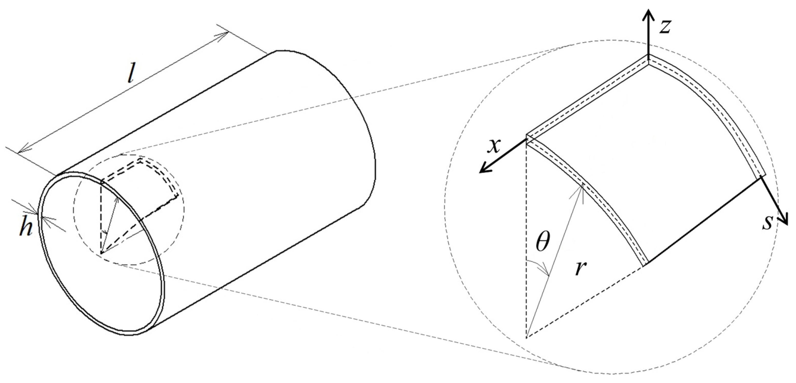
2. Equations of Motion for Thin Circular Cylindrical Shells

Consider an isotropic and homogeneous thin circular cylindrical shell with length l , uniform thickness h , mean radius r , Young’s modulus E , Poisson’s ratio ν , and density ρ . Figure 1 shows the coordinate system defined for the middle surface by the axial direction x , the circumferential direction s , and the radial direction z . θ is the angular circumferential coordinate.
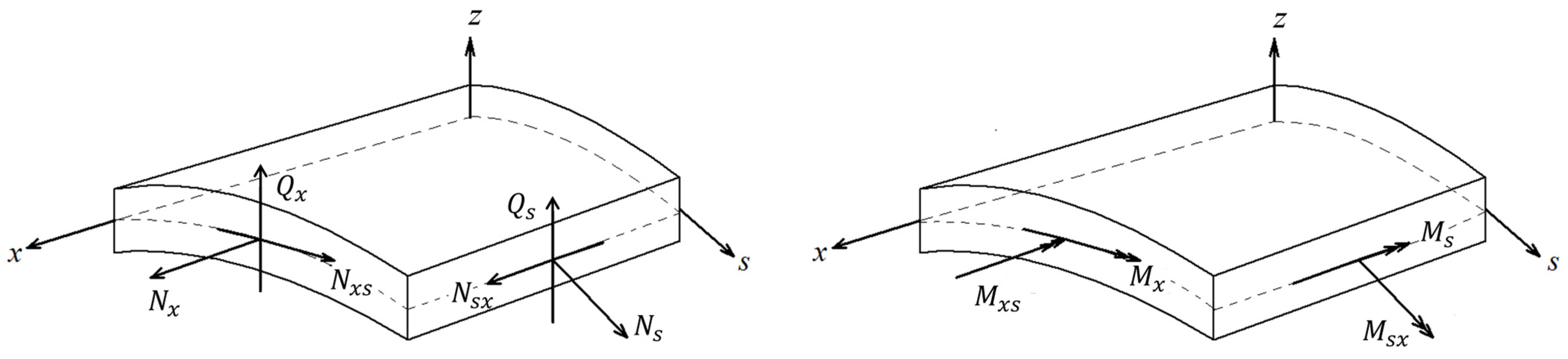
Considering a differential element of the cylindrical shell, the positive forces and moments acting per unit length are shown in Figure 2. For the face with normal along the x direction, N x and N x s are the in-plane normal and shear forces, Q x is the out-of-plane shear force, a n d   M x and M x s are the bending moment and torsional moment. The same considerations are valid, respectively, for N s , N s x , Q s , M s x , and M s for the face with normal along the s direction.
The cylindrical shell theory adopted in the present research and outlined in this section is the Donnell–Mushtari version of Love’s theory.
The resulting equations of motion derived from the translational equilibrium along x , s , and z are as follows:
N x x + N s x s = ρ h d 2 u x d t 2 N s s + N x s x = ρ h d 2 u s d t 2 Q s s + Q x x N s r = ρ h d 2 u z d t 2
From the rotational equilibrium with respect to x and s , the relations between the transverse shear force resultants and the moment resultants reduce to:
M s s + M x s x Q s = 0 M x x + M s x s Q x = 0
By substituting Equation (2) into the last of Equation (1), the latter reduces to:
2 M x x 2 + 2 2 M x s x s + 2 M s s 2 N s r = ρ h d 2 u z d t 2
The strain–displacement relations are:
ε x = u x x ε s = u s s + u z r γ x s = u s x + u x s k x = 2 u z x 2 k s = 2 u z s 2 τ = 2 2 u z x s
where u x , u s , and u z are the displacement components of a point on the middle surface along the axial, circumferential, and radial directions; ε x and ε s are the normal strains along x and s directions; γ x s is the in-plane shear strain; k x and k s are the changes in the curvature of the mid-surface; and τ is the mid-surface twist. Note that ε r = γ s r = γ x r = 0 for Love’s hypotheses.
Lastly, the resultants of forces and moments are related to the stresses, which in turn are related to the strains by Hooke’s law. Hence, the resulting forces and moments are reduced to the following functions of strains:
N x = K ε x + ν ε s N s = K ε s + ν ε x N x s = N s x = K 1 ν 2 γ x s M x = D k x + ν k s M s = D k s + ν k x M x s = M s x = K 1 ν 2 τ
where K = E h 1 ν 2 and D = E h 3 12 ( 1 ν 2 ) are, respectively, the tensile and bending stiffness of the cylindrical shell.
After substituting the strain–displacement relation of Equation (4) into Equation (5) and then introducing the latter into the first two equations of motion of Equation (1) and in Equation (3), considering that d s = r · d θ , the final equations of motion expressed as functions of displacements are:
K 2 u x x 2 + 1 ν 2 r 2 2 u x θ 2 + 1 + ν 2 r 2 u s x θ + ν r u z x = ρ h d 2 u x d t 2 K 1 r 2 2 u s θ 2 + 1 ν 2 2 u s x 2 + 1 + ν 2 r 2 u x x θ + 1 r 2 u z θ = ρ h d 2 u s d t 2 K ν r u x x 1 r 2 u s θ u z r 2 h 2 12 4 u z x 4 + 1 r 4 4 u z θ 4 + 2 r 2 4 u z x 2 θ 2 = ρ h d 2 u z d t 2
Equation (6) constitute an eighth-order system of coupled partial differential equations in terms of the three displacement components. Under the hypothesis of a small thickness, the dependence of the three displacement components from the radial coordinate can be neglected; thus, the general expression of the eigenfunctions of the problem is:
u x = F x x , θ , t u s = F s ( x , θ , t ) u z = F z ( x , θ , t )
where t is the time coordinate. Four boundary conditions for each cylinder end must be introduced to solve the problem. Nevertheless, an exact solution is not available in an explicit form for any combination of boundary constraints. Thus, an approximated resolution based on an energetic method is described in the next section.

3. Generalised Eigenvalue Problem for Natural Frequencies

The most common methods to simplify the free vibrations problem of thin-walled cylinders are based on energetic variational approaches similarly to the Rayleigh–Ritz method. The system of partial differential equations derived from the fundamental theories of thin cylindrical shells (Equation (6)) is reduced to a simpler system of ordinary differential equations by assuming reasonable eigenfunctions for the three displacement components so as not to violate the end conditions, and introducing the equations of motion and the assumed eigenfunctions in an energetic principle. Hence, the resulting solution is not exact but approximately correct on the whole domain.
From the experimental evidence, each vibrational mode of a cylindrical shell is characterised by the number of transverse half-waves, denoted by the positive integer m , and the number of circumferential waves, indicated by the positive integer n . The relevant literature reports several applications proving that fairly accurate results are achieved if a particular solution for a given mode, identified by specific m and n values, is derived by performing a variables separation in the displacements eigenfunctions while ensuring the compliance with the end conditions and the periodicity of the circumferential waveform. Thus, the three coordinates x , θ , and t can be decoupled as follows:
u x ( x , θ , t ) = A x d F m X d X cos n θ cos ω t u s ( x , θ , t ) = A s F m X sin n θ cos ω t u z x , θ , t = A z F m X cos n θ cos ω t
where X = x / l is the axial coordinate normalised to the cylinder length; A x , A s , and A z are constant displacement amplitudes; and F m X is the m th transverse waveform of a beam constrained as the cylinder under analysis, which can be generalised as:
F m X = C 1 cos β m X + C 2 cosh β m X + C 3 sin β m X + C 4 sinh β m X
where C 1 , C 2 , C 3 , and C 4 are constant values depending on m and the boundary constraints. For a simply supported end, the latter result in the following conditions is:
u s = u z = N x = M x = 0
For a clamped end, it is:
u x = u s = u z = u z x = 0
Table 1 lists the flexural waveforms and the frequency equations for a beam subject to the boundary conditions of interest, which are well-established in the relevant literature [20]. For given constraints, each m th waveform of the beam depends on the m th root of the transcendental frequency equation, denoted by β m . Note that the transverse waveform is the same for both ends clamped or one clamped and one simply supported, but the frequency equation and the related solutions differ.
At this point, the equations of motion of Equation (6) are introduced in the principle of virtual work, according to which the virtual work δ W of all the forces acting on the system, including the inertial actions, is null for any virtual displacements δ u x , δ u s , and δ u z that do not violate the boundary conditions:
δ W = r K 0 2 π 0 l 2 u x x 2 + 1 ν 2 r 2 2 u x θ 2 + 1 + ν 2 r 2 u s x θ + ν r u z x 1 ν 2 E   ρ d 2 u x d t 2 δ u x + 1 r 2 2 u s θ 2 + 1 ν 2 2 u s x 2 + 1 + ν 2 r 2 u x x θ + 1 r 2 u z θ 1 ν 2 E ρ d 2 u s d t 2 δ u s ν r u x x + 1 r 2 u s θ + u z r 2 + h 2 12 4 u z x 4 + 1 r 4 4 u z θ 4 + 2 r 2 4 u z x 2 θ 2 + 1 ν 2 E ρ d 2 u z d t 2 δ u z d x d θ = 0
Given the arbitrariness of the virtual displacements δ u x , δ u s , and δ u z , Equation (12) can be satisfied if each of the three addends is null. Thus, the problem is reduced to the following three-equation system, obtained by normalising to the cylinder length l :
0 2 π 0 1 2 u x X 2 + 1 ν 2 R 2 2 u x 2 + 1 + ν 2 R 2 u s X θ + ν R u z X 1 ν 2 E ρ l 2 d 2 u x d t 2 δ u x d X d θ = 0 0 2 π 0 1 1 R 2 2 u s θ 2 + 1 ν 2 2 u s X 2 + 1 + ν 2 R 2 u x X θ + 1 R 2 u z θ 1 ν 2 E ρ l 2 d 2 u s d t 2 δ u s d X d θ = 0 0 2 π 0 1 ν R u x X + 1 R 2 u s θ + u z R 2 + H 2 12 4 u z X 4 + 1 R 4 4 u z θ 4 + 2 R 2 4 u z X 2 θ 2 + 1 ν 2 E ρ l 2 d 2 u z d t 2 δ u z d X d θ = 0
where R = r / l is the cylinder mean radius normalised to the length and H = h / l is the normalised thickness.
The system of Equation (13) can be reduced by introducing the assumed eigenfunctions of Equation (8) for the displacement components and their partial derivatives. In particular, consider that for each displacement component d 2 u i d t 2 = ω 2 u i and δ u i = δ A i u i / A i where δ A i is arbitrary, the reduced system does not depend on the time coordinate t ; indeed, each term of the equations would be multiplied by cos 2 ω t , which is constant within the integration domain and thus can be simplified. Moreover, the dependence on the circumferential coordinate θ can also be eliminated, because it reduces to 0 2 π cos 2 n θ d θ = π for the first and the third equation and to 0 2 π sin 2 n θ d θ = π for the second one. Hence, after some mathematical manipulation, Equation (13) is reduced to the following homogeneous linear system:
I 13 A x 1 ν 2 R 2 n 2 I 11 A x + 1 + ν 2 R n I 11 A s + ν R I 11 A z +   I 11 A x = 0 n 2 R 2 I 00 A s + 1 ν 2 I 02 A s 1 + ν 2 R n I 02 A x n R 2 I 00 A z +   I 00 A s = 0 ν R I 02 A x + n R 2 I 00 A s + 1 R 2 I 00 A z + H 2 12 I 04 A z + n 4 R 4 I 00 A z 2 n 2 R 2 I 02 A z   I 00 A z = 0
where = 1 ν 2 E ρ l 2 ω 2 . The notation I i j is the definite integral from 0 to 1 of the product between the i th- and j th-order derivatives of the function F m X for a given number m of flexural half-waves:
I i j = 0 1 d i d X i F m X · d j d X j F m X d X f o r   i = 0,1   a n d   j = 0,1 , 2,3 , 4
The zero-order derivative is the function F m X itself.
After simple mathematical manipulation, Equation (14) reduces to the following matrix formulation:
D   ̿ I ̿   A = 0
where A = { A x ; A s ; A z } is the unknown vector containing the displacements amplitudes in the three directions, I ̿ is the identity matrix, and D ̿ is the following matrix:
D ̿ = I 13 I 11 + 1 ν 2 R 2 n 2 n 1 + ν 2 R ν R 1 + ν 2 n R I 02 I 00 1 ν 2 I 02 I 00 + n 2 R 2 n R 2 ν R I 02 I 00 n R 2 1 R 2 + H 2 12 I 04 I 00 + n 4 R 4 2 R 2 n 2 I 02 I 00
As it is apparent from Equation (16), the natural frequency of any thin-walled cylinder can be easily calculated by solving the eigenvalue problem of the matrix D ̿ , which, thus, is equivalent to a typical dynamic matrix in the modal analysis of discreet systems. From the three eigenvalues 1 , 2 , and 3 , the natural frequency is obtained as follows:
f i = 1 2 π E i 1 ν 2 ρ l 2 f o r   i = 1 ,   2 ,   3
The eigenvectors corresponding to each eigenvalue determine the ratios between the amplitude of the axial, circumferential, and radial displacements for any mode shape.
It is crucial to notice that the integrals of Equation (15) are univocally defined only by the specific m and the cylinder boundary conditions because of the normalisation to the cylinder length. Moreover, from Equations (9) and (15), it can be easily derived that:
I 04 I 00 = β m 4
where β m can be derived from Table 1. Hence, only the following ratios must be calculated:
I 13 I 11 = 0 1 d F m X d X · d 3 F m X d X 3 d X 0 1 d F m X d X 2 d X I 02 I 00 = 0 1 F m X · d 2 F m X d X 2 d X 0 1 F m 2 X d X
Table 2, Table 3 and Table 4 list the values of interest of Equation (20), which are derived from the beam flexural waveforms of Table 1 for the corresponding end condition and can be used in Equation (17) for any thin cylindrical shell.
As a result, populating the dynamic matrix D ̿ and solving its eigenvalue problem is immediate and straightforward once the cylinder geometry ( R , H , l ), the material properties ( ν , E , ρ ), the vibrational mode ( m , n ), and the end constraints (Table 2, Table 3 and Table 4) are known.

4. Results and Discussion

The procedure described in Section 3 was carried out for cylinders with different geometry and material under the three end conditions of interest, i.e., two simply supported ends, two clamped ends, and one clamped and one simply supported end. The eigenvalue problem for the dynamic matrix D ̿ was performed in MATLAB R2022a numerical software.
Firstly, the natural frequencies and the displacement amplitudes’ ratios of a steel cylinder ( ρ = 7833 kg/m3, E = 207 kN/mm2, ν = 0.3) with mean radius r = 76 mm, length l = 305 mm, and thickness h = 0.254 mm were assessed in the three scenarios. The trend of the resulting natural frequencies agrees with the vibrational behaviour of thin-walled cylinders predicted by the relevant literature [11,15,16,17,29,33,35,46,50,52,54,56]; therefore, the results of this first analysis, discussed in Section 4.1, are listed in the Appendix A. On the contrary, the numerical and graphical results presented in the current section focus on the model validation.
The same steel cylinder defined above was considered to test the model accuracy by assuming the results of an FEM analysis as a benchmark, as addressed in Section 4.2. Section 4.3 proposes a sensitivity analysis of the present model with respect to cylinder geometry and material, presenting a validity range whereby the maximum error against FEM is approximately 10%. Lastly, Section 4.4 compares the present model with the results obtained by some experimental, numerical, and analytical methods available in the literature.
For Section 4.1, Section 4.2 and Section 4.3, all the mode shapes with m 8 and n 14 were examined. Nonetheless, the natural frequencies for m > 4 are not listed in the Appendix A and in Section 4.2 for brevity, but the general considerations made in Section 4.1 and Section 4.2 remain valid also for m 4 . Moreover, as it is common in the literature on the topic, only the first natural frequency is considered for the model validation carried out in Section 4.2, Section 4.3 and Section 4.4, being the lowest natural frequency as it is addressed in Section 4.1, and thus the one to be monitored to prevent the undesired risk of resonance phenomena.

4.1. Natural Frequencies and Amplitude Ratios

Table A1, Table A2 and Table A3 list the results for the natural frequencies associated with each mode shape ( m , n ) for every boundary condition derived from the eigenvalues of the dynamic matrix. It is apparent that the first frequency f 1 is lower than f 2 and f 3 by up to two orders of magnitude. Moreover, it is worth noting that f 2 and f 3 are monotonically increasing for increasing m and n , while f 1 shows a minimum for a number n of circumferential waves that increases with the considered number m of transverse half-waves. In Table A1, Table A2 and Table A3, the minimum value of f 1 for a given number m of transverse half-waves is underlined. This general trend for the frequency f 1 was explained by Arnold and Warburton in [11] by the opposite variation of the stretching energy, which decreases with the number of circumferential waves, and the bending energy, which, on the contrary, increases; as a result, the minimum of the lowest natural frequency f 1 for a given number m of transverse half-waves is due to a minimum in the total strain energy. Nonetheless, depending on the cylinder geometry, f 1 can show a monotonic trend for a low number of transverse half-waves. The global minimum of f 1 , highlighted in bold in Table A1, Table A2 and Table A3, occurs for m = 1 and n = 5 if the cylinder has one or two simply supported ends; instead, it occurs for m = 1 and n = 6 for the clamped/clamped cylinder. Furthermore, for each mode shape ( m , n ), the natural frequencies of the clamped/simply supported cylinder (Table A3) are intermediate between those of the simply supported/simply supported cylinder (Table A1), which are the lowest, and clamped/clamped cylinder (Table A2), which are the highest. This evidence validates the hypothesis that the natural frequencies of any cylinder under an arbitrary degree of fixing lie between the natural frequencies achieved for simply supported and clamped ends [14], corroborating the generality of this work.
Table A4, Table A5 and Table A6 show the amplitude ratios derived from the eigenvectors of each mode shape only for n 7 , for brevity. The amplitude of the radial displacement A z is chosen as the normalising term. The predominant motion associated with the frequency f 1 is the radial one, while the circumferential displacement and, above all, the axial displacement are small. Thus, the first frequency implies a transverse vibrational mode, whose displacement amplitude increases for increasing m and n . On the contrary, for f 2 and f 3 , the amplitude of the radial displacement decreases for increasing m and n . Nonetheless, for the second frequency f 2 , A x grows faster than A s for m = 1; thus, an axial motion is predominant for any n for a simply supported/simply supported cylinder, n 4 for a clamped/clamped cylinder, and n 3 for a clamped/simply supported cylinder. For m 2, f 2 mainly involves a predominant circumferential motion. The third frequency f 3 is always associated with a predominant circumferential motion. Similar trends were obtained in [46] for the amplitude ratios of a clamped/clamped cylinder.

4.2. Comparison with FEM Results

To test the accuracy of the novel approximated method, the results of a simulations campaign carried out in the commercial software Ansys 22.1, based on the finite element method, were considered as a benchmark. For this purpose, SHELL181 linear elements were used for the modal analysis. Table 5, Table 6 and Table 7 compare the first frequency f 1 obtained by the approximated method and the FEM analysis, reporting the percentage error between the two approaches. Overall, for the cylinder with two simply supported ends, the error is far lower than ± 1% and mainly negative, which means that the first natural frequency is slightly underestimated on average. On the contrary, the error is higher and mainly positive for the other two end conditions. In Table 5, Table 6 and Table 7, the error related to the global minimum of f 1 is underlined in bold, while an asterisk indicates the maximum error. In this regard, the maximum error between the fast approximated method and the FEM for the simply supported/simply supported cylinder is 2.07% and occurs for m = 1 and n = 6 ; instead, the maximum error is 9.82% and 11.9% for the clamped/clamped or clamped/simply supported cylinder, respectively; in both cases, it occurs for m = n = 1 . Nonetheless, the error occurring for the global minimum frequency, the most potentially dangerous, is just 2.01%, 3.05%, and 3.66%, respectively. Therefore, the level of accuracy is satisfactory.
Figure 3 graphically summarises the results of the comparison with the FEM analysis, showing the trend of f 1 for m 8 and n 14. The minimum value of f 1 for each m is indicated by a black dot.

4.3. Influence of Cylinder Geometry and Material on Model Accuracy

To further explore the potentiality of the model, its accuracy was tested for different cylinder geometry and material within m 8 and n 14. Starting from the reference steel cylinder with l / r = 4 and h / r = 1/300, cylinder length and thickness were changed in turn to assess how they affect model performance for any boundary condition. The observed ranges of variation are 2 l / r 10 and 1/400 h / r 1/20. For this purpose, it was sufficient to accordingly change R or H in the dynamic matrix D ̿ and repeat the resolution of the eigenvalue problem. FEM simulations were conducted to obtain the benchmark values for the first frequency f 1 .
Table 8 lists the acceptable range of variation of l / r and h / r to comply with a maximum error of the model against the FEM results of approximately 10%. It also reports the maximum error for the global minimum frequency observed within the acceptable range. For any boundary conditions, the model accuracy increases for thinner cylinders. All other conditions being equal, the maximum acceptable value of the thickness/radius ratios is higher for the simply supported/simply supported cylinder, accordingly to the higher model accuracy observed for this boundary condition. On the contrary, the model accuracy improves for long cylinders with two clamped ends and for short cylinders with two simply supported ends. This trend affects the accuracy for a clamped/simply supported cylinder, which shows an intermediate behaviour. Even though the acceptable ranges listed in Table 8 involve a maximum error of approximately 10%, the error related to the global minimum frequency is approximately 5% only.
Table 9 compares the maximum error and the error for the lowest f 1 for a steel and an aluminium cylinder ( ρ = 2700 kg/m3, E = 68.2 kN/mm2, ν = 0.33) with r = 76 mm, l = 305 mm, a n d   h = 0.254 mm. There are no significant differences, suggesting that the model performance is not affected by the cylinder material.

4.4. Comparison with the Literature

A further test on the validity of the proposed model is performed by considering data available in the literature. This section compares several experimental, numerical, and analytical methods of simply supported/simply supported and clamped/clamped thin-walled cylinders. Different cylinder geometry and material are considered. Experimental or FEM results are always assumed as the benchmark to assess the percentage difference. For brevity, when results for different numbers of transverse half-waves were available, the numerical values listed in the tables reported in the remainder of the section are generally those for m = 1, whereby the lowest frequencies are observed. The clamped/simply supported condition is not considered here due to the lack of FEM and experimental data in the literature. Table 10 summarises the literature comparison.
The natural frequencies of an aluminium simply supported/simply supported cylinder were experimentally assessed by Sewall and Naumann [15] in 1968. After that, the same cylinder was considered by Naeem and Sharma [50] to present a procedure based on the Rayleigh–Ritz variational approach. The transverse waveforms are modelled by Ritz polynomial functions, resulting in the formulation of an eigenvalue problem which is rather cumbersome, requiring analytical integrations and differentiations. The experimental results were available for m = 1 and 4 n 13. Figure 4 shows the results of the comparison. From the numerical comparison reported in Table 11, the maximum percentage difference of the present model against the experimental data is 4.30% for n = 13, while Naeem and Sharma’s model shows a maximum difference of −4.81% for n = 6. The error in the global minimum frequency for n = 7 is −0.36% for the present model and 1.64% for Naeem and Sharma. Other experimental results were formerly obtained by Arnold and Warburton [11] in 1949 for a steel simply supported/simply supported cylinder. Results were available for m 10 and 2 n 6. From Table 12, which reports the results of the comparison for m 4 for brevity, the maximum percentage difference, observed for the global minimum frequency, is 16.22% for m = 1 and n = 2. Complete results are shown in Figure 5.
A comparison with the results reported by Pellicano [29] is presented in Table 13 and Table 14, and Figure 6 for an aluminium cylinder with two simply supported ends and two clamped ends, respectively. Pellicano’s model assumes Chebyshev polynomials for eigenfunctions and requires a numerical technique for the resolution. Data were available for m = 1 and 5 n 12 for the simply supported/simply supported cylinder and for m = 1 and 6 n 13 for the clamped/clamped cylinder. The percentage error is assessed against the results of an FEM analysis performed by Pellicano. For the cylinder with two simply supported ends, the exact solution is also provided. In this case, the results of Pellicano’s numerical method equal the exact solution; nonetheless, the present model shows a maximum error of only 0.92% for n = 8 against FEM and 1.76% for n = 9 against the exact solution. The error in the global minimum frequency for n = 7 is 0.73% against FEM and −0.06% against the exact solution. Concerning the clamped/clamped cylinder, Table 14 shows that the present model has a maximum error of 6.04% for n = 6, where Pellicano’s method has a maximum error of 1.02%; however, the error of the present model in the global minimum frequency for n = 9 equals 2.88%, while Pellicano has an error of 0.34%. The error is still good, given the greater simplicity of the proposed novel formulation.
Xuebin [54] used the wave propagation method and introduced the flexural vibrational mode of a beam to obtain a noniterative mathematical resolution based on a third-order equation. The natural frequencies for an aluminium clamped/clamped cylinder for m = 1, 3, 5, and n 10 were assessed. Table 15 shows the comparison with the present model only for m = 1 for brevity, but complete results are shown in Figure 7. The error is assessed with respect to the results of an FEM analysis reported by Xuebin. The error in the global minimum frequency for n = 4 is 8.22% for the present model against 1.16% for Xuebin. However, Xuebin’s method shows a significant error for a low number of circumferential waves, achieving a maximum error of 36.19% for n = 1, more than three times higher than the maximum error of the present model equal to 10.04%. Moreover, the calculation of the coefficients of the third-order equation underpinning Xuebin’s approach is rather convoluted in comparison to the present approximated model.
The last comparison is with the experimental data of Koval and Cranch [16], the analytical closed-form approaches of Wang and Lai [53] and Moazzez et al. [56], the exact solution of Xing et al. [33] numerically evaluated, and the FEM results discussed in Section 4.2. Wang and Lai used a direct formula derived from the free vibrations of an infinite-length cylinder. Moazzez et al. used a cascaded algebraic resolution of a third-order equation, presented by Cammalleri and Costanza in [46], that distinguishes different coefficients for even and odd numbers of transverse half-waves. Xing et al. used the Donnell–Mushtari equations without any other simplifying assumption; thus, the solution is “exact” but assessed by Newton’s iterative method. Table 16 lists the first natural frequency assessed for m = 1 and n 8. The present method and the one used by Moazzez et al. are in very good agreement, showing a maximum error lower than 10% for n = 1 and an error of approximately 3% in the global minimum frequency for n = 6. The “exact” solution of Xing et al. shows the least error with respect to the FEM and experimental data. Against FEM, the maximum error against FEM of Xing et al. is −3.97% for n = 2, while the error in the global minimum frequency is −0.02%. Nonetheless, the higher error of the present model in comparison with Xing et al. is still acceptable, given the straightforward practice use of the present method that requires neither any initial guess frequencies nor a convergence analysis of the solving algorithm, unlike Xing et al. The approximated formula proposed by Wang and Lai is the less accurate, especially for lower n . It has a maximum error against FEM of 39.47% for n = 1 and an error in the global minimum frequency of 2.59%. Figure 8 shows the available first natural frequencies of the models under considerations for m 4. Moazzez’s results were excluded from the graphical comparison because they are almost the same as those obtained by the present model.
Overall, the comparison presented in this section suggests that the numerical methods achieve more accurate results, especially with two clamped edges, but at the expense of fast usability. On the contrary, the present approximated model offers a swift, straightforward mathematical treatment which leads to satisfactory accuracy, especially if compared to other analytical methods that sometimes fail for a low number of circumferential waves. The error for the global minimum frequency is generally much lower than 10%. Hence, the practical interest of the proposed approach is significant, given that its ease of use is hard to find in the relevant literature, especially for cylinders with one or two clamped ends. Moreover, it should be noted that, for a given absolute difference, the percentage error is higher for lower frequencies because of its own definition. Indeed, the graphical comparisons of Figure 4, Figure 5, Figure 6, Figure 7 and Figure 8 show that the trend of the results obtained by the novel approximated model is in good agreement with FEM and experimental data, even when the percentage error in the global minimum is numerically higher.
When assessing the outcomes of the above comparisons, it should be considered that they may have been affected by potential errors in the results chosen as the benchmark. For instance, the fact that the frequencies resulting from experimental data are often lower than those numerically or analytically assessed suggests that the stiffness of the experimental set-up is lower than those theoretically predicted. Also, potential measurement errors may have occurred. Similarly, the goodness of the results of FEM analysis is strictly dependent on the mesh quality and elements number and type. Therefore, the errors of the present model are widely acceptable within the unavoidable uncertainty range of any engineering problem.

5. Conclusions

This paper proposed a novel procedure to study the free vibrations of an isotropic circular cylindrical shell under different boundary conditions.
The cylinder equations of motion of Donnell–Mushtari’s shell theory were introduced in the principle of virtual work. The normalisation of the resulting system to the cylinder length and the introduction of the eigenfunction of a beam as constrained as the cylinder led to a significant simplification of the mathematical treatment, which was reduced to the eigenvalue problem of a 3 × 3 matrix. In other words, the problem of the free vibrations of a continuous system was reduced to the straightforward definition of a dynamic matrix depending on the cylinder geometry, material, and end constraints, similarly to the modal analysis of discreet systems.
The natural frequencies for several simply supported/simply supported, clamped/clamped, and clamped/simply supported cylinders were assessed and compared to FEM results, experimental data available in the literature, and other numerical and analytical methods. The vibrational behaviour of the clamped/simply supported cylinder lies between the double-simply supported condition, which implies the lowest frequencies, and the double-clamped condition, which results in the highest frequencies. For the cylinder proposed as a case study, the comparison with the present model and FEM analysis showed very good accuracy for a cylinder with two simply supported ends, involving a maximum error of 2.07%. This error increases with one or two clamped ends up to 11.9% and 9.82%, respectively. Nonetheless, the error occurring for the global minimum frequency, the most potentially dangerous, is just 2.01%, 3.66%, and 3.05%, respectively.
To provide a broader insight into the model validity, an FEM simulation campaign proved that the maximum error of approximately 10% for any combination of m and n is achievable for a wide range of cylinder geometry for any considered end condition. Within the assessed validity range, the error for the global minimum frequency is approximately 5% only. Moreover, a literature comparison showed that the present model resulted in comparable or even higher accuracy than other approximated closed-form approaches available in the literature, while the “exact” methods relying on more cumbersome and time-consuming iterative and numerical techniques perform better, at the expense of usability and immediacy of the computing procedure. Therefore, in general, the level of accuracy is excellent, given that the exact solution of the free vibrations problem for the clamped-end constraints does not exist in a closed form. Thus, the practical interest of the present model is significant.
To conclude, the proposed novel model proved to be a reliable, easy-to-use tool suitable for the rapid esteem of natural frequencies of thin-walled cylinders subject to simply supported or clamped-end conditions. The main strength is the excellent trade-off between usability and accuracy, making it easily implementable also in the design stage without requiring a deep knowledge of the topic.

Author Contributions

Conceptualization, M.C.; methodology, M.C.; software, A.C.; validation, A.C. and M.C.; investigation, A.C.; writing—original draft preparation, A.C.; writing—review and editing, M.C. and A.C.; visualization, A.C.; supervision, M.C. All authors have read and agreed to the published version of the manuscript.

Funding

This research received no external funding.

Data Availability Statement

Not applicable.

Conflicts of Interest

The authors declare no conflict of interest.

Nomenclature

r cylinder mean radius
A x , A s , A z displacements amplitude
D bending stiffness of the cylindrical shell
D ̿ cylinder dynamic matrix
E Young’s modulus
f 1 , f 2 , f 3 natural frequencies
F m beam transverse waveform with m half-waves
h cylinder thickness
k x , k s changes in the curvature of the mid-surface of the cylinder
K tensile stiffness of the cylindrical shell
l cylinder length
m number of transverse half-waves
M x , M x s , M s x , M s moments per unit length
n number of circumferential waves
N x , N x s , N s , N s x in-plane normal and shear forces per unit length
Q x , Q s transverse shear forces per unit length
z radial coordinate
s circumferential coordinate
t time coordinate
u x , u s , u z components of displacement of a point on the cylinder mid-surface
W virtual work
x axial coordinate
X axial coordinate normalised to the cylinder length
R mean radius normalised to the cylinder length
γ x s in-plane shear strain
ε x , ε s normal strains
H thickness normalised to the cylinder length
θ angular circumferential coordinate
ν Poisson’s ratio
ρ density
τ cylinder mid-surface twist
ω 1 , ω 2 , ω 3 natural circular frequency

Appendix A

Table A1. Natural frequencies for a cylinder with two simply supported ends for m 4 and n 14 ( r = 76 mm, l = 305 mm, h = 0.254 mm, ρ = 7833 kg/m3, E = 207 kN/mm2, ν = 0.3). The minimum values of the first frequency f 1 for a given m are underlined. The global minimum frequency is highlighted in bold.
n m = 1 m = 2 m = 3 m = 4
f 1 (Hz) f 2 (Hz) f 3 (Hz) f 1 (Hz) f 2 (Hz) f 3 (Hz) f 1 (Hz) f 2 (Hz) f 3 (Hz) f 1 (Hz) f 2 (Hz) f 3 (Hz)
1288610,00917,209644514,05921,944855617,89029,228952722,35437,344
2126514,88926,403367718,06129,947582121,64735,508734425,58142,338
365620,92336,632217823,19439,414389626,22243,820541329,71249,482
442327,31947,298139629,01249,558268131,49153,176398634,51857,937
537233,84758,18398535,17760,072193137,22563,123299439,83367,200
643140,43369,19079241,52370,807147743,24973,434232345,50976,983
755147,04880,27275147,97181,681122749,45583,983188451,43487,115
870553,68191,40381954,48192,649113255,78094,694162657,53397,491
988760,325102,56695661,031103,683115862,184105,520151663,753108,044
10109266,976113,753113967,607114,764127268,644116,431152670,063118,728
11132073,632124,958135574,203125,881144975,144127,405163076,438129,511
12157080,291136,175159980,814137,024167081,675138,428180382,863140,371
13184286,954147,403186787,434148,189192488,228149,490202889,327151,293
14213593,618158,639215994,063159,370220894,800160,582229295,821162,263
Table A2. Natural frequencies for a cylinder with two clamped ends for m 4 and n 14 ( r = 76 mm, l = 305 mm, h = 0.254 mm, ρ = 7833 kg/m3, E = 207 kN/mm2, ν = 0.3). The minimum values of the first frequency f 1 for a given m are underlined. The global minimum frequency is highlighted in bold.
n m = 1 m = 2 m = 3 m = 4
f 1 (Hz) f 2 (Hz) f 3 (Hz) f 1 (Hz) f 2 (Hz) f 3 (Hz) f 1 (Hz) f 2 (Hz) f 3 (Hz) f 1 (Hz) f 2 (Hz) f 3 (Hz)
1378815,18420,252693316,67027,457878119,73535,709967023,86544,181
2208420,42827,371432022,40632,787619225,05439,893755528,32247,661
3123325,54837,098279327,79040,930436030,50946,555572333,46853,269
480631,11847,592190133,23950,501314235,94054,947434838,78460,588
560537,02658,396137538,93060,735234241,48164,358336044,20769,108
655543,15069,358107744,84371,312182147,19574,356266149,76878,415
761149,41480,41094350,92482,089150053,07484,708218155,47788,235
873655,77391,52093857,12992,991133559,09495,289187361,32798,400
990362,197102,668102763,425103,977130065,225106,023171167,299108,803
10110268,670113,844118369,789115,022136971,446116,866167273,373119,377
11132675,177125,039138376,205126,111151377,736127,788173679,532130,078
12157481,712136,250161882,661137,233171484,082138,771187985,760140,873
13184588,268147,471188189,149148,379195690,474149,800208392,046151,743
14213894,841158,702217095,662159,545223196,903160,865233498,380162,671
Table A3. Natural frequencies for a clamped/simply supported cylinder for m 4 and n 14 ( r = 76 mm, l = 305 mm, h = 0.254 mm, ρ = 7833 kg/m3, E = 207 kN/mm2, ν = 0.3). The minimum values of the first frequency f 1 for a given m are underlined. The global minimum frequency is highlighted in bold.
n m = 1 m = 2 m = 3 m = 4
f 1 (Hz) f 2 (Hz) f 3 (Hz) f 1 (Hz) f 2 (Hz) f 3 (Hz) f 1 (Hz) f 2 (Hz) f 3 (Hz) f 1 (Hz) f 2 (Hz) f 3 (Hz)
1348512,71317,907672015,63324,262867618,94332,238960323,18240,619
2173717,08426,746404020,31031,068602623,49737,427745727,07544,796
395722,60936,848251225,36740,048414928,39245,006558031,67451,192
460928,65547,454166130,93049,977292833,64453,962418036,66359,134
547634,94458,305118336,84460,380214639,23263,687318741,97568,072
648241,36069,29093242,97971,048165345,08173,865249947,55977,648
757447,85180,35784249,25681,879136451,11984,329203753,35887,643
871754,38791,47687355,62792,818123257,29394,982175159,32397,925
989360,955102,63198862,063103,829122663,566105,766161365,417108,410
10109667,544113,812115868,545114,894131869,912116,646159871,609119,044
11132274,150125,011136875,062125,997147976,314127,596168177,879129,788
12157280,767136,224160781,605137,130169082,760138,599184084,209140,619
13184387,393147,448187488,168148,286193989,239149,645205490,588151,516
14213794,027158,680216494,747159,459221995,745160,724231297,006162,466
Table A4. Displacement amplitudes’ ratios for a cylinder with two simply supported ends for m 4 and n 7 ( r = 76 mm, l = 305 mm, h = 0.254 mm, ρ = 7833 kg/m3, E = 207 kN/mm2, ν = 0.3).
n m =  1 m =  2
f 1 f 2 f 3 f 1 f 2 f 3
A x / A z A s / A z A x / A z A s / A z A x / A z A s / A z A x / A z A s / A z A x / A z A s / A z A x / A z A s / A z
10.0981.010.710.310.201.180.0170.720.211.180.361.72
20.0450.511.280.840.222.150.0210.480.401.380.292.60
30.0240.342.281.370.233.120.0160.340.661.730.273.47
40.0140.253.701.900.244.100.0110.251.022.150.264.38
50.00940.205.522.410.245.080.00800.201.482.610.265.32
60.00670.177.762.930.246.070.00590.172.033.090.256.27
70.00490.1410.403.440.257.060.00450.142.693.570.257.23
n m =  3 m =  4
f 1 f 2 f 3 f 1 f 2 f 3
A x / A z A s / A z A x / A z A s / A z A x / A z A s / A z A x / A z A s / A z A x / A z A s / A z A x / A z A s / A z
10.00140.420.142.450.522.250.00370.240.134.420.622.60
20.00790.390.242.120.373.210.00210.300.183.130.463.83
30.00910.310.362.260.314.000.00460.270.252.970.374.62
40.00780.250.522.560.294.820.00500.230.353.110.335.38
50.00630.200.732.940.285.690.00460.200.463.380.306.18
60.00500.170.973.360.276.590.00390.170.603.730.297.03
70.00400.151.273.800.267.520.00330.140.774.120.287.90
Table A5. Displacement amplitudes’ ratios for a cylinder with two clamped ends for m 4 and n 7 ( r = 76 mm, l = 305 mm, h = 0.254 mm, ρ = 7833 kg/m3, E = 207 kN/mm2, ν = 0.3).
n m =  1 m =  2
f 1 f 2 f 3 f 1 f 2 f 3
A x / A z A s / A z A x / A z A s / A z A x / A z A s / A z A x / A z A s / A z A x / A z A s / A z A x / A z A s / A z
10.0260.910.221.020.881.410.00570.640.0971.520.871.92
20.0220.490.891.550.412.250.0110.450.271.940.522.83
30.0150.331.851.940.323.170.0100.320.542.310.383.62
40.0110.253.062.350.284.130.00820.250.882.680.324.48
50.00780.204.572.790.275.110.00640.201.303.070.295.39
60.00580.176.383.250.266.090.00500.171.793.490.286.33
70.00450.148.523.710.267.080.00400.142.363.930.277.28
n m =  3 m =  4
f 1 f 2 f 3 f 1 f 2 f 3
A x / A z A s / A z A x / A z A s / A z A x / A z A s / A z A x / A z A s / A z A x / A z A s / A z A x / A z A s / A z
10.00140.380.0772.630.912.270.00260.230.0774.460.922.51
20.00420.370.162.550.623.450.00110.280.123.450.693.99
30.00570.300.292.810.454.220.00300.260.203.450.524.86
40.00550.240.453.120.374.990.00350.220.303.650.425.60
50.00480.200.653.470.335.820.00350.190.413.930.376.36
60.00410.170.893.840.306.690.00320.160.554.260.337.17
70.00340.141.164.240.297.600.00280.140.714.620.318.02
Table A6. Displacement amplitudes’ ratios for a clamped/simply supported cylinder for m 4 and n 7 ( r = 76 mm, l = 305 mm, h = 0.254 mm, ρ = 7833 kg/m3, E = 207 kN/mm2, ν = 0.3).
n m =  1 m =  2
f 1 f 2 f 3 f 1 f 2 f 3
A x / A z A s / A z A x / A z A s / A z A x / A z A s / A z A x / A z A s / A z A x / A z A s / A z A x / A z A s / A z
10.0510.950.530.720.311.250.00960.680.151.390.561.82
20.0330.501.131.130.272.190.01520.460.351.680.372.70
30.0200.342.021.580.263.150.01280.330.612.010.313.54
40.0130.253.242.060.254.120.00970.250.962.390.284.43
50.00880.204.812.550.255.100.00720.201.382.820.275.35
60.00630.176.733.040.256.080.00550.171.903.270.266.30
70.00480.149.003.530.257.070.00430.142.513.730.267.26
n m =  3 m =  4
f 1 f 2 f 3 f 1 f 2 f 3
A x / A z A s / A z A x / A z A s / A z A x / A z A s / A z A x / A z A s / A z A x / A z A s / A z A x / A z A s / A z
10.00150.400.102.540.702.270.00310.240.104.420.762.55
20.00570.380.202.360.483.330.00150.290.153.310.563.92
30.00720.310.332.550.374.100.00370.270.233.220.444.74
40.00660.240.492.840.324.900.00420.230.323.390.375.48
50.00550.200.693.190.305.750.00400.190.443.650.336.27
60.00450.170.933.580.286.640.00350.170.583.980.317.09
70.00370.141.214.010.277.560.00300.140.744.360.297.96

References

  1. Hemmer, M.; Van Khang, H.; Robbersmyr, K.G.; Waag, T.I.; Meyer, T.J.J. Fault Classification of Axial and Radial Roller Bearings Using Transfer Learning through a Pretrained Convolutional Neural Network. Designs 2018, 2, 56. [Google Scholar] [CrossRef]
  2. Awada, A.; Younes, R.; Ilinca, A. Optimized Active Control of a Smart Cantilever Beam Using Genetic Algorithm. Designs 2022, 6, 36. [Google Scholar] [CrossRef]
  3. Love, A.E.H. The Small Free Vibrations and Deformation of a Thin Elastic Shell. Philos. Trans. R. Soc. Lond. 1888, 179, 491–546. [Google Scholar] [CrossRef]
  4. Flügge, W. Stresses in Shells; Springer: Berlin/Heidelberg, Germany, 1962; ISBN 3662010283. [Google Scholar]
  5. Timoshenko, S.; Woinowsky-Krieger, S. Theory of Plates and Shells; McGraw Hill: New York, NY, USA, 1959; Volume 2. [Google Scholar]
  6. Sanders, J.L., Jr. An Improved First-Approximation Theory for Thin Shells; US Government Printing Office: Washington, DC, USA, 1959; p. 1.
  7. Reissner, E. A New Derivation of the Equations for the Deformation of Elastic Shells. Am. J. Math. 1941, 63, 177. [Google Scholar] [CrossRef]
  8. Donnell, L.H. Beams, Plates and Shells; McGraw-Hill: New York, NY, USA, 1976; ISBN 0070175934. [Google Scholar]
  9. Mushtari, K.M. Certain Generalizations of the Theory of Thin Shells. Izv. Fiz. Mat. Ob-va. Pri Kaz. Un-te 1938, 11, 28–56. [Google Scholar]
  10. Leissa, A.W. Vibration of Shells; Scientific and Technical Information Office, National Aeronautics and Space Administration: Washington, DC, USA, 1973; Volume 288.
  11. Arnold, R.N.; Warburton, G.B. Flexural Vibrations of the Walls of Thin Cylindrical Shells Having Freely Supported Ends. Proc. R. Soc. Lond. Ser. A Math. Phys. Sci. 1949, 197, 238–256. [Google Scholar] [CrossRef]
  12. Warburton, G.B. Vibration of Thin Cylindrical Shells. J. Mech. Eng. Sci. 1965, 7, 399–407. [Google Scholar] [CrossRef]
  13. Strutt, J.W.; Rayleigh, J.W.S.B. The Theory of Sound; Macmillan: New York, NY, USA, 1894; Volume 1. [Google Scholar]
  14. Arnold, R.N.; Warburton, G.B. The Flexural Vibrations of Thin Cylinders. Proc. Inst. Mech. Eng. 1953, 167, 62–80. [Google Scholar] [CrossRef]
  15. Sewall, J.L.; Naumann, E.C. An Experimental and Analytical Vibration Study of Thin Cylindrical Shells with and without Longitudinal Stiffeners; National Aeronautic and Space Administration: Washington, DC, USA, 1968; Volume 4705.
  16. Koval, L.R.; Cranch, E.T. On the Free Vibration of Thin Cylindrical Shells Subjected to an Initial Static Torque. Proc. 4th U.S. Natl. Congr. Appl. Mech. 1962, 1, 107–117. [Google Scholar]
  17. Smith, B.L.; Haft, E.E. Natural Frequencies of Clamped Cylindrical Shells. AIAA J. 1968, 6, 720–721. [Google Scholar] [CrossRef]
  18. Sharma, C.B.; Johns, D.J. Vibration Characteristics of a Clamped-Free and Clamped-Ring-Stiffened Circular Cylindrical Shell. J. Sound Vib. 1971, 14, 459–474. [Google Scholar] [CrossRef]
  19. Sharma, C.B. Free Vibrations of Clamped-Free Circular Cylinders. Thin-Walled Struct. 1984, 2, 175–193. [Google Scholar] [CrossRef]
  20. Blevins, R.D. Formulas for Natural Frequency and Mode Shape; Van Nostrand Reinhold Co.: New York, NY, USA, 1979. [Google Scholar]
  21. Soedel, W. Vibrations of Shells and Plates, 3rd ed.; Marcel Dekker: New York, NY, USA, 2004. [Google Scholar]
  22. El-Mously, M. Fundamental Natural Frequencies of Thin Cylindrical Shells: A Comparative Study. J. Sound Vib. 2003, 264, 1167–1186. [Google Scholar] [CrossRef]
  23. Forsberg, K. A Review of Analytical Methods Used to Determine the Modal Characteristics of Cylindrical Shells; NASA: Washington, DC, USA, 1966.
  24. Santiago, J.M.; Wisniewski, H.L. Convergence of Finite Element Frequency Predictions for a Thin Walled Cylinder. Comput. Struct. 1989, 32, 745–759. [Google Scholar] [CrossRef]
  25. Chung, H. Free Vibration Analysis of Circular Cylindrical Shells. J. Sound Vib. 1981, 74, 331–350. [Google Scholar] [CrossRef]
  26. Bert, C.W.; Malik, M. Free Vibration Analysis of Thin Cylindrical Shells by the Differential Quadrature Method. J. Press. Vessel Technol. 1996, 118, 1–12. [Google Scholar] [CrossRef]
  27. Loy, C.T.; Lam, K.Y.; Shu, C. Analysis of Cylindrical Shells Using Generalized Differential Quadrature. Shock Vib. 1997, 4, 193–198. [Google Scholar] [CrossRef]
  28. Zhang, L.; Xiang, Y.; Wei, G.W. Local Adaptive Differential Quadrature for Free Vibration Analysis of Cylindrical Shells with Various Boundary Conditions. Int. J. Mech. Sci. 2006, 48, 1126–1138. [Google Scholar] [CrossRef]
  29. Pellicano, F. Vibrations of Circular Cylindrical Shells: Theory and Experiments. J. Sound Vib. 2007, 303, 154–170. [Google Scholar] [CrossRef]
  30. Xuebin, L. A New Approach for Free Vibration Analysis of Thin Circular Cylindrical Shell. J. Sound Vib. 2006, 296, 91–98. [Google Scholar] [CrossRef]
  31. Khalili, S.M.R.; Davar, A.; Malekzadeh Fard, K. Free Vibration Analysis of Homogeneous Isotropic Circular Cylindrical Shells Based on a New Three-Dimensional Refined Higher-Order Theory. Int. J. Mech. Sci. 2012, 56, 1–25. [Google Scholar] [CrossRef]
  32. Xie, X.; Jin, G.; Liu, Z. Free Vibration Analysis of Cylindrical Shells Using the Haar Wavelet Method. Int. J. Mech. Sci. 2013, 77, 47–56. [Google Scholar] [CrossRef]
  33. Xing, Y.; Liu, B.; Xu, T. Exact Solutions for Free Vibration of Circular Cylindrical Shells with Classical Boundary Conditions. Int. J. Mech. Sci. 2013, 75, 178–188. [Google Scholar] [CrossRef]
  34. Fakkaew, W.; Cole, M.O.T.; Chamroon, C. On the Vibrational Dynamics of Rotating Thin-Walled Cylinders: A Theoretical and Experimental Study Utilizing Active Magnetic Bearings. Int. J. Mech. Sci. 2019, 163, 105101. [Google Scholar] [CrossRef]
  35. Rawat, A.; Matsagar, V.A.; Nagpal, A.K. Free Vibration Analysis of Thin Circular Cylindrical Shell with Closure Using Finite Element Method. Int. J. Steel Struct. 2020, 20, 175–193. [Google Scholar] [CrossRef]
  36. Tang, D.; Wu, G.; Yao, X.; Wang, C. Free Vibration Analysis of Circular Cylindrical Shells with Arbitrary Boundary Conditions by the Method of Reverberation-Ray Matrix. Shock Vib. 2016, 2016, 3814693. [Google Scholar] [CrossRef]
  37. Kumar, A.; Das, S.L.; Wahi, P. Effect of Radial Loads on the Natural Frequencies of Thin-Walled Circular Cylindrical Shells. Int. J. Mech. Sci. 2017, 122, 37–52. [Google Scholar] [CrossRef]
  38. Tong, Z.Z.; Ni, Y.W.; Zhou, Z.H.; Xu, X.S.; Zhu, S.B.; Miao, X.Y. Exact Solutions for Free Vibration of Cylindrical Shells by a Symplectic Approach. J. Vib. Eng. Technol. 2018, 6, 107–115. [Google Scholar] [CrossRef]
  39. Jia, J.; Lai, A.; Li, T.; Zhou, Z.; Xu, X.; Lim, C.W. A Symplectic Analytical Approach for Free Vibration of Orthotropic Cylindrical Shells with Stepped Thickness under Arbitrary Boundary Conditions. Thin-Walled Struct. 2022, 171, 108696. [Google Scholar] [CrossRef]
  40. Borković, A.; Radenković, G.; Majstorović, D.; Milovanović, S.; Milašinović, D.; Cvijić, R. Free Vibration Analysis of Singly Curved Shells Using the Isogeometric Finite Strip Method. Thin-Walled Struct. 2020, 157, 107125. [Google Scholar] [CrossRef]
  41. Li, H.; Pang, F.; Miao, X.; Gao, S.; Liu, F. A Semi Analytical Method for Free Vibration Analysis of Composite Laminated Cylindrical and Spherical Shells with Complex Boundary Conditions. Thin-Walled Struct. 2019, 136, 200–220. [Google Scholar] [CrossRef]
  42. Liew, K.M.; Hu, Y.G.; Ng, T.Y.; Zhao, X. Dynamic Stability of Rotating Cylindrical Shells Subjected to Periodic Axial Loads. Int. J. Solids Struct. 2006, 43, 7553–7570. [Google Scholar] [CrossRef]
  43. Rizzetto, F.; Jansen, E.; Strozzi, M.; Pellicano, F. Nonlinear Dynamic Stability of Cylindrical Shells under Pulsating Axial Loading via Finite Element Analysis Using Numerical Time Integration. Thin-Walled Struct. 2019, 143, 106213. [Google Scholar] [CrossRef]
  44. Ng, T.Y.; Lam, K.Y.; Liew, K.M.; Reddy, J.N. Dynamic Stability Analysis of Functionally Graded Cylindrical Shells under Periodic Axial Loading. Int. J. Solids Struct. 2001, 38, 1295–1309. [Google Scholar] [CrossRef]
  45. Weingarten, V.I. Free Vibration of Thin Cylindrical Shells. Aiaa J. 2012, 2, 717–722. [Google Scholar] [CrossRef]
  46. Cammalleri, M.; Costanza, A. A Closed-Form Solution for Natural Frequencies of Thin-Walled Cylinders with Clamped Edges. Int. J. Mech. Sci. 2016, 110, 116–126. [Google Scholar] [CrossRef]
  47. Cammalleri, M.; Castellano, A.; Abella, M. A Simple Tool to Forecast the Natural Frequencies of Thin-Walled Cylinders. Mater. Res. Proc. 2023, 26, 635–640. [Google Scholar] [CrossRef]
  48. Yang, Y.; Wei, Y. A Unified Approach for the Vibration Analysis of Cylindrical Shells with General Boundary Conditions. Acta Mech. 2018, 229, 3693–3713. [Google Scholar] [CrossRef]
  49. Sorge, F.; Cammalleri, M. On the Beneficial Effect of Rotor Suspension Anisotropy on Viscous-Dry Hysteretic Instability. Meccanica 2012, 47, 1705–1722. [Google Scholar] [CrossRef]
  50. Naeem, M.N.; Sharma, C.B. Prediction of Natural Frequencies for Thin Circular Cylindrical Shells. Proc. Inst. Mech. Eng. Part C J. Mech. Eng. Sci. 2000, 214, 1313–1328. [Google Scholar] [CrossRef]
  51. Qin, Z.; Chu, F.; Zu, J. Free Vibrations of Cylindrical Shells with Arbitrary Boundary Conditions: A Comparison Study. Int. J. Mech. Sci. 2017, 133, 91–99. [Google Scholar] [CrossRef]
  52. Ji, M.; Inaba, K.; Triawan, F. Vibration Characteristics of Cylindrical Shells Filled with Fluid Based on First-Order Shell Theory. J. Fluids Struct. 2019, 85, 275–291. [Google Scholar] [CrossRef]
  53. Wang, C.; Lai, J.C.S. Prediction of Natural Frequencies of Finite Length Circular Cylindrical Shells. Appl. Acoust. 2000, 59, 385–400. [Google Scholar] [CrossRef]
  54. Xuebin, L. Study on Free Vibration Analysis of Circular Cylindrical Shells Using Wave Propagation. J. Sound Vib. 2008, 311, 667–682. [Google Scholar] [CrossRef]
  55. Zhang, X.M.; Liu, G.R.; Lam, K.Y. Vibration Analysis of Thin Cylindrical Shells Using Wave Propagation Approach. J. Sound Vib. 2001, 239, 397–403. [Google Scholar] [CrossRef]
  56. Moazzez, K.; Saeidi Googarchin, H.; Sharifi, S.M.H. Natural Frequency Analysis of a Cylindrical Shell Containing a Variably Oriented Surface Crack Utilizing Line-Spring Model. Thin-Walled Struct. 2018, 125, 63–75. [Google Scholar] [CrossRef]
  57. Ramezani, H.; Mirzaei, M. Transient Elastodynamic Behavior of Cylindrical Tubes under Moving Pressures and Different Boundary Conditions. Appl. Math. Model. 2020, 77, 934–949. [Google Scholar] [CrossRef]
Figure 1. Geometry and coordinate system on the mid-surface for a thin-walled cylinder.
Designs 07 00122 g001
Figure 2. Positive forces and moments acting on a differential element.
Designs 07 00122 g002
Figure 3. Comparison between the novel model and FEM analysis for any boundary condition. The present results are represented by continuous lines; FEM results are represented by X markers and dotted lines; a black dot indicates the minimum frequency for a given m .
Designs 07 00122 g003
Figure 4. Comparison between the present model, Naeem and Sharma’s model [50], and experimental data from Sewall and Neumann [15] (Exp.) for m = 1.
Designs 07 00122 g004
Figure 5. Comparison between the present model and the experimental results of Arnold and Warburton [11] for m 8. The present results are represented by continuous lines; the experimental data are represented by X markers and dotted lines.
Designs 07 00122 g005
Figure 6. Comparison between the present model and Pellicano’s numerical and FEM results [29] for m = 1.
Designs 07 00122 g006
Figure 7. Comparison between the present model and Xuebin’s analytical and FEM results [54] for m = 1, 3, and 5.
Designs 07 00122 g007
Figure 8. Comparison among the present model, the analytical closed-form approaches of Wang and Lai [53], the numerical solution of Xing et al. [33], the experimental data of Koval and Cranch [16] (Exp.), and FEM results.
Designs 07 00122 g008
Table 1. Flexural waveforms of a beam as a function of the normalised axial coordinate X = x / l for different constraints. C m is an arbitrary amplitude constant.
Boundary ConditionsFrequency EquationRoots of Frequency EquationFlexural Waveform
Simply supp./Simply supp. sin β m = 0 β m = m π for m = 1,2 , 3 , F m X = C m sin β m X
Clamped/Clamped cos β m cosh β m = 1 β 1 = 4.73004
β 2 = 7.85320
β m = 2 m + 1 π 2 for m 3
F m X = C m cos β m X cosh β m X cos β m cosh β m sin β m sinh β m sin β m X sinh β m X
Clamped/Simply supported tan β m tanh β m = 0 β 1 = 3.92660
β 2 = 7.06858
β m = 4 m + 1 π 4 for m 3
F m X = C m cos β m X cosh β m X cos β m cosh β m sin β m sinh β m sin β m X sinh β m X
Table 2. Numerical values for integrals ratios for any cylinder with two simply supported ends for m 8 .
m = 1 m = 2 m = 3 m = 4 m = 5 m = 6 m = 7 m = 8
I 13 I 11 −9.870−39.478−88.826−157.914−246.740−355.306−483.611−631.655
I 02 I 00 −9.870−39.478−88.826−157.914−246.740−355.306−483.611−631.655
Table 3. Numerical values for integrals ratios for any cylinder with two clamped ends for m 8 .
m = 1 m = 2 m = 3 m = 4 m = 5 m = 6 m = 7 m = 8
I 13 I 11 −40.688−82.596−147.795−232.792−337.637−462.266−606.660−770.810
I 02 I 00 −12.303−46.050−98.905−171.586−263.998−376.150−508.041−659.673
Table 4. Numerical values for integrals ratios for any clamped/simply supported cylinder for m 8 .
m = 1 m = 2 m = 3 m = 4 m = 5 m = 6 m = 7 m = 8
I 13 I 11 −20.649−58.198−115.566−192.702−289.589−406.220−542.594−698.708
I 02 I 00 −11.513−42.896−94.038−164.918−255.538−365.896−495.995−645.832
Table 5. First natural frequency f 1 assessed by the present model and FEM modal analysis and percentage error. Results for a steel cylinder with two simply supported ends for m 4 and n 14 . The error for the global minimum is underlined in bold; an asterisk indicates the maximum error.
n m = 1 m = 2 m = 3 m = 4
f 1 (Hz)Error (%) f 1 (Hz)Error (%) f 1 (Hz)Error (%) f 1 (Hz)Error (%)
PresentFEMPresentFEMPresentFEMPresentFEM
12885.892885.9−0.00046444.76445.3−0.0108555.78557.3−0.0189527.59529.5−0.021
21265.131265.00.0113676.63677.5−0.0255820.85823.2−0.0437344.47348.5−0.055
3656.0654.80.192178.12178.8−0.0343896.13898.9−0.0715413.05418.2−0.096
4422.7418.70.961396.41396.30.00932681.12683.5−0.0923986.13991.5−0.14
5372.0364.72.01985.3983.50.181931.41933.0−0.0822994.22999.2−0.17
6431.4422.62.07 *792.1788.10.511477.21477.4−0.0132322.62326.7−0.18
7550.6542.21.56751.4745.70.761226.61225.20.121884.41887.3−0.15
8705.3698.21.02818.6812.70.721131.61129.00.231626.41628.0−0.10
9886.7881.80.56955.9951.50.471157.81155.30.211515.71516.8−0.072
101091.91090.10.171138.91137.30.151272.51271.80.0481525.71527.6−0.12
111319.71322.2−0.181355.21357.7−0.181448.91451.8−0.201629.61634.1−0.28
121569.71577.7−0.511599.01607.0−0.501669.51677.7−0.491803.01812.1−0.50
131841.61856.9−0.821867.41882.6−0.811924.41939.5−0.782027.92043.6−0.77
142135.52159.9−1.132159.22183.5−1.112207.92232.1−1.092292.52316.9−1.05
Table 6. First natural frequency f 1 assessed by the present model and FEM modal analysis and percentage error. Results for a steel cylinder with two clamped ends for m 4 and n 14 . The error for the global minimum is underlined in bold; an asterisk indicates the maximum error.
n m = 1 m = 2 m = 3 m = 4
f 1 (Hz)Error (%) f 1 (Hz)Error (%) f 1 (Hz)Error (%) f 1 (Hz)Error (%)
PresentFEMPresentFEMPresentFEMPresentFEM
1378834509.82 *693365246.27878187590.25967096440.28
2208419964.40432039459.50619259753.62755575300.32
3123311854.09279325559.30436041096.10572355782.59
48067694.79190118522.67314229476.63434841734.20
56055814.11137513114.84234222086.07336032024.91
65555383.05107710363.94182118090.69266125434.65
76116001.889439162.92150014652.39218120964.04
87367290.979389211.75133513111.8318731930−2.94
99038970.71102710151.26130012761.94171116692.49
10110210990.25118311760.57136913541.10167216461.61
1113261328−0.13138313820.071151315070.42173617210.84
1215741582−0.4616181623−0.3317141715−0.11187918750.21
1318451860−0.7818811894−0.6819561966−0.5320832090−0.30
1421382162−1.0921702192−1.0122312251−0.9023342351−0.73
Table 7. First natural frequency f 1 assessed by the present model and FEM modal analysis and percentage error. Results for a steel clamped/simply supported cylinder for m 4 and n 14 . The error for the global minimum is underlined in bold; an asterisk indicates the maximum error.
n m = 1 m = 2 m = 3 m = 4
f 1 (Hz)Error (%) f 1 (Hz)Error (%) f 1 (Hz)Error (%) f 1 (Hz)Error (%)
PresentFEMPresentFEMPresentFEMPresentFEM
13485311511.88 *672064494.21867685581.38960395320.75
2173716028.40404038135.97602658512.98745773531.42
39579045.87251223785.63414939913.96558054512.36
46095834.52166115884.60292828163.96418040632.87
54764603.66118311413.66214620743.49318730972.89
64824692.729329062.88165316072.89249924352.62
75745641.828428252.13136413332.29203719922.22
87177091.148738611.41123212121.68175117211.75
98938880.629889800.81122612131.0816131665−3.13
10109610940.21115811550.33131813110.54159815930.29
1113221324−0.1513681369−0.073147914780.08168116770.26
1215721579−0.4816071614−0.4216901695−0.3118401843−0.16
1318431858−0.7918741888−0.7519391952−0.6720542066−0.55
1421372161−1.1021642187−1.0622192241−1.0023122333−0.90
Table 8. Results of the sensitivity analysis for a different cylinder length and thickness; the acceptable range provides an error within 10%.
Boundary Conditions Influence   of   l / r Influence   of   h / r
Acceptable Range Error   for   Minimum   f 1 Acceptable Range Error   for   Minimum   f 1
Simply supp./Simply supp. l / r 104.54% h / r 1/204.92%
Clamped/Clamped l / r 3.33.83% h / r 1/1005.46%
Clamped/Simply supported l / r   2.4   and   l / r 64.58% h / r 1/1005.28%
Table 9. Results of the sensitivity analysis for a different cylinder material.
Boundary ConditionsSteelAluminium
Maximum Error Error   for   Minimum   f 1 Maximum Error Error   for   Minimum   f 1
Simply supp./Simply supp.2.07%2.01%2.07%4.92%
Clamped/Clamped9.82%3.05%9.82%5.46%
Clamped/Simply supported11.88%3.66%11.88%5.28%
Table 10. Summary of the literature comparison.
ReferenceMethodBoundary ConditionsCylinder MaterialCylinder Geometry
Sewall and Naumann [15]experimentalSimply supp./Simply supp.aluminium:
ρ = 2715 kg/m3, E = 69 kN/mm2, ν = 0.315
r = 242.3 mm,
l = 609.6 mm, h = 0.648 mm
Naeem and Sharma [50]analytical
Arnold and Warburton [11]experimentalSimply supp./Simply supp.steel:
ρ = 7833 kg/m3, E = 207 kN/mm2, ν = 0.29
r = 48.9 mm, l = 397 mm,
h = 2.5654 mm
Pellicano [29]numericalSimply supp./Simply supp.aluminium:
ρ = 2796 kg/m3, E = 71 kN/mm2, ν = 0.31
r = 100 mm, l = 200 mm,
h = 0.247 mm
Clamped/Clamped
Xuebin [54]analyticalClamped/Clampedaluminium:
ρ = 2700 kg/m3, E = 64.7 kN/mm2, ν = 0.329
r = 153.5 mm, l = 800 mm, h = 1.1016 mm
Koval and Cranch [16]experimentalClamped/Clampedsteel:
ρ = 7833 kg/m3, E = 207 kN/mm2, ν = 0.3
r = 76 mm, l = 305 mm,
h = 0.254 mm
Xing et al. [33]numerical
Wang and Lai [53]analytical
Moazzez et al. [56]analytical
Table 11. Comparison among the present model, Naeem and Sharma’s model [50] (N&S), and experimental data from Sewall and Neumann [15] (Exp.) for m = 1 for an aluminium simply supported/simply supported cylinder. The error for the global minimum is underlined in bold; an asterisk indicates the maximum error.
n f 1 (Hz)Error (%)
PresentN&S [50]Exp. [15]Present vs. Exp.N&S vs. Exp.
42882882870.350.21
5203202203−0.11−0.57
6168167175−3.89−4.81 *
71681661690.361.64
81921891882.000.67
92292272242.451.29
102772742664.043.03
113313293261.630.80
123923893851.871.17
134594564404.30 *3.68
Table 12. Comparison between the present model and experimental data from Arnold and Warburton [11] (Exp.) for a steel simply supported/simply supported cylinder. The error for the global minimum is underlined in bold; an asterisk indicates the maximum error.
n m = 1 m = 2 m = 3 m = 4
f 1 (Hz)Error (%) f 1 (Hz)Error (%) f 1 (Hz)Error (%) f 1 (Hz)Error (%)
PresentExp. [11]PresentExp. [11]PresentExp. [11]PresentExp. [11]
2111696016.22 *220720706.62394337255.865831527010.64
3231021308.44259624207.29330231305.49437341804.62
4414939854.11429741304.04461844304.25515849504.21
5652864002.01665265002.34688267002.72724170303.01
6943992701.83955893702.00976495702.0310,06898502.22
Table 13. Comparison between the present model and the results reported by Pellicano [29] for m = 1 for an aluminium simply supported/simply supported cylinder. The error for the global minimum is underlined in bold; an asterisk indicates the maximum error.
n f 1 (Hz)Error (%)
PresentPellicano [29]Exact [29]FEM [29]Present vs. FEMPellicano vs. FEMPresent vs. Exact
57247227227230.14−0.060.20
65565535535540.39−0.070.47
74884854854850.730.060.79
84944904904900.92 *−0.081.00
95525425425470.89−0.86 *1.76 *
106436376376380.74−0.170.92
117577517517520.58−0.210.79
128888828828850.41−0.270.69
Table 14. Comparison between the present model and the results reported by Pellicano [29] for m = 1 for an aluminium clamped/clamped cylinder. The error for the global minimum is underlined in bold; an asterisk indicates the maximum error.
n f 1 (Hz)Error (%)
PresentPellicano [29]FEM [29]Present vs. FEMPellicano vs. FEM
69869409306.04 *1.02 *
78147827755.020.88
87257026973.960.63
97056886852.880.34
107427287271.970.10
118208098101.31−0.06
129309219220.87−0.18
131063105510570.61−0.19
Table 15. Comparison between the present model and the results reported by Xuebin [54] for m = 1 for an aluminium clamped/clamped cylinder. The error for the global minimum is underlined in bold; an asterisk indicates the maximum error.
n f 1 (Hz)Error (%)
PresentXuebin [54]FEM [54]Present vs. FEMXuebin vs. FEM
113281644120710.04 *36.19 *
26807606327.6220.17
33934073686.7010.54
42952762738.221.16
53202962919.921.84
64163823789.920.85
75525075049.430.49
87156586568.980.31
99038338318.640.18
101114102910288.380.08
Table 16. Comparison among the present model and the results of Koval and Cranch [16] (Exp.), Wang and Lai [53] (W&L), Moazzez et al. [56], and Xing et al. [33] for m = 1 for a steel clamped/clamped cylinder. The error against FEM for the global minimum is underlined in bold; an asterisk indicates the maximum error.
n f 1 (Hz)Error (%)
PresentMoazzez [56]W&L [53]Xing [33]Exp.
[16]
FEMPresent/Moazzez vs. FEMW&L vs. FEMXing
vs. FEM
Present/Moazzez vs. Exp.W&L vs. Exp.Xing
vs. Exp.
13788379048113425-34509.82 *39.47 *−0.71---
22084208524521917-19964.4022.84−3.97 *---
31233123413561154102511854.0914.44−2.6120.33 *32.29 *12.59 *
48068078477647007694.7910.07−0.7115.1921.009.14
56056056155805595814.115.83−0.198.2310.023.76
65555555525385255383.052.590.025.625.142.48
76116116055985876001.880.83−0.344.143.071.87
87367367287237207290.97−0.13−0.812.221.110.42
Disclaimer/Publisher’s Note: The statements, opinions and data contained in all publications are solely those of the individual author(s) and contributor(s) and not of MDPI and/or the editor(s). MDPI and/or the editor(s) disclaim responsibility for any injury to people or property resulting from any ideas, methods, instructions or products referred to in the content.

