Article

Designing Power Transformer Using Particle Swarm Optimization with Respect to Transformer Noise, Weight, and Losses

1
Department of Electrical and Information Engineering, Universitas Gadjah Mada Yogyakarta, Yogyakarta 55281, Indonesia
2
Department of Electrical Engineering, Universitas Islam Indonesia Yogyakarta, Yogyakarta 55584, Indonesia
3
Elsewedy Electric Indonesia, Bogor Regency 16820, Indonesia
4
Faculty of Electricity and Renewable Energy, Institute of Technology PLN, Jakarta 11750, Indonesia
*
Authors to whom correspondence should be addressed.
Designs 2023, 7(1), 31; https://doi.org/10.3390/designs7010031
Submission received: 14 November 2022 / Revised: 7 February 2023 / Accepted: 8 February 2023 / Published: 10 February 2023

Abstract

:
The increased use of electrical energy will encourage the installation of more power transformers in residential areas as well as in industrial areas. Each power transformer, in its operation, will generate noise that can interfere with comfort and, at some level, cause health problems. The design of the power transformer currently focuses on optimizing its economic side, so noise has not been considered at this design stage. This research is about optimizing the low noise transformer design. The main goal is to obtain a low noise power transformer with low production costs. The method used in this optimization is particle swarm optimization with a multi-objective function. The objective function consists of the minimization of load noise, core weight, and winding weight. In this study, 11 optimized variables were used. Some variables that are optimized must be in the form of integers. Therefore, the optimization process needs a mechanism for mapping variables. The results showed that a low noise power transformer could be designed at optimal cost. Design validation was performed analytically and numerically with COMSOL software. The optimization results showed a decrease in load noise, core, and winding weight by 0.86 dB, 2.12%, and 47.46%, respectively. The results of this optimization are better than the designs used regularly in the industry.

1. Introduction

A power transformer is an essential tool in the electric power system. The power transformer is a static electrical device consisting of one, two, or more windings coupled with or without a magnetic core to connect electrical circuits [1]. The primary role of these devices is to transmit electrical energy from one voltage level to another without changing the frequency [2,3].
The increasing demand for electrical energy will encourage the installation of more power transformers in residential areas [4] and industrial environments. Each power transformer, in operation, will generate noise in the form of a sound or buzzing sound [5], which will change based on the size of the load. Noise is unwanted sound from a business or activity at a certain level and time that can cause disturbances to human health and environmental comfort [6]. The noise level standard is the maximum level of noise allowed to be discharged into the environment from a business or activity so that it does not cause human health problems and environmental discomfort [6]. Public awareness of environmental issues has been highlighted [7] and must be considered by energy providers and power transformer companies that use and produce power transformers with low noise [8,9].
The primary noise sources from a power transformer are the magnetic core, windings [5,8], and the cooling system [7,10,11]. Noise originating from the core of the power transformer is caused by the maxwell force [12,13] and magnetostriction [5,10,12], which is the change in the shape of the core material due to exposure to changing magnetic flux [10]. The noise frequency generated from this magnetostriction process is twice the source frequency. The non-linear nature of the magnetostriction causes higher even-order harmonics to appear as a result of core vibrations [11]. The noise from the windings is caused by the interaction between the current flowing in the windings and the leaky flux that hits it, causing the Lorentz force [11,14]. The noise caused by the transformer windings due to the load current is called load noise. No-load noise is a summation of noise caused by the transformer core and the cooling system. Meanwhile, total noise is a combination of all noise components generated, namely no-load noise, load noise, and noise from the cooling device.
Optimizing any power transformer design is a complex task because it must meet the standards and specifications set by consumers to keep production costs low. The development of modern transformers has led to smaller dimensions and cheaper production costs while maintaining high energy efficiency. The main objective in power transformer design optimization is to obtain the lowest production costs (material, labor, and overhead costs) [15] and the lowest total loss and owning costs [16,17] while maintaining the highest technical specifications. The design methodology will depend on the type of transformer (distribution, power or instrumentation), its operation frequency, the core construction’s characteristics, the cooling method or the type of magnetic material [18].
Aspects considered in transformer design include [19]: no-load loss, load loss, short circuit impedance, inrush current, dynamic behavior when a short circuit occurs, noise, isolation, and cooling system. So far, the design of the transformer has focused more on optimizing production costs by minimizing material costs without leaving the desired loss limit in designing power transformers.
Aspect load noise is rarely considered in power transformer designs. The problem occurs when the load noise generated by the power transformer exceeds the specifications determined by the consumer. Efforts to reduce load noise by adding dampers will increase production costs, dimensions, and weight of transformers.
Therefore, in this study, a power transformer design optimization method is proposed by including the load noise aspect as one of the objective functions, in addition to the material core and winding weight. The optimization method uses particle swarm optimization (PSO) by modifying the optimized variable mapping process. The PSO method is a method that is easy to implement and quick to get a solution.

2. Materials and Methods

The design of the power transformer includes the design of the core, the design of windings on the low-voltage side and the high-voltage side, the design of tanks and the design of cooling systems. An essential part of the design’s focus is the core and winding designs. This focus is because the highest cost of the material comes from the core and winding. In this study, the steps and equations in the design of power transformers are based on [18].

2.1. The Core Design

The core in a three-phase power transformer usually has three limbs and two yokes. Within this core are laid high-voltage and low-voltage windings, and the yokes serve as a pathway for the flow of magnetic flux. The limbs for power transformers are usually arranged in a step-like pattern to get a nearly circular shape for the lowest possible regression. The number of steps is determined based on the amount of power from the transformer, which is proportional to the gross section area of the transformer core. The basic dimensions of the transformer core are the diameter of the limbs, the window’s height and width, the distance between the centers of the limb, the height of the yoke and the cross-sectional area of the limbs and yokes.
The phase voltage per turn of the winding is defined by (1). Meanwhile, the cross-sectional area of the limb and the relationship between the phase voltage per turn, frequency, and density of maximum magnetic flux is specified by (2).
E t = K t S
A c = E t 4.44   f   B m
A constant value of the turns ratio ( K t ) for a three-phase power transformer is between 0.4 and 0.7. The diameter of the core is expressed by (3).
d c = 2 K s A c π
The value of the space factor, K s , usually has a value of 0.9.

2.2. Low Voltage (LV) Winding Design

The number of turns in LV winding ( N LV ) compares phase voltage to voltage per turn, expressed by (4).
N LV = V LV E t
while the phase current on LV winding ( I LV ) for delta connection is expressed by (5).
I LV = S 3   V LV
The cross-sectional area per turn for LV winding ( A L V ) is determined by (6).
A LV = I LV δ LV
with δ L V as the current density of LV winding. Overall LV winding width ( w L V ) is defined by (7).
w LV = w LV 1 × n _ R LV × n _ L D LV
with w LV 1 as the thickness of one LV winding conductor with its insulation, n _ R LV as the number of LV winding conductors radially per turn, and n _ L D LV as the number of turns per disk for LV winding. The height of LV winding can be derived from (8).
h LV = ( h LV 1 + d _ D LV × n _ D LV ) d _ D LV
with h LV 1 as the height of one disk of LV winding (consisting of more than one axially arranged conductor) with its insulation, d _ D LV distance between disks axially, n _ D LV as the number of LV winding disks. LV winding consists of several parallel conductors to reduce eddy loss. The thickness and width of each conductor must withstand the force caused by a short circuit and keep the disk in a stable condition.

2.3. High Voltage (HV) Winding Design

In the same way, the HV winding parameter can be determined by (9) to (14), starting from the current per phase ( I HV ) (star connection), the number of turns in HV winding ( N HV ), cross-sectional area per turn for HV winding ( A HV ), the width of HV winding ( w HV ), and height of HV winding ( h HV ).
I HV = S   V HV 3
N HV = V HV E t 3
A HV = w HV 1 × t HV × n _ R HV × n _ A HV
  δ HV = I HV A HV
w HV = w HV 1 × n _ R HV × n _ L D HV
h HV = ( h HV 1 + d _ D HV × n _ D HV ) d _ D HV
with   δ HV as the current density of HV winding, w HV 1 as the thickness of one HV winding conductor with its insulation,   t HV as the width of one HV winding conductor, n _ R HV as the number of HV winding conductors radially per turn and n _ L D HV as the number of turns per disk for HV winding, h HV 1 as the height of one turn of HV winding (may consist of more than one axially arranged conductor) with its insulation, d _ D HV distance between disks axially, n _ D HV as the number of HV winding disks.
The height of HV winding is not much different from that of LV winding to maintain magnetic balance in the winding. Therefore, determining the number of disks and turns per disk needs to be optimized while meeting the minimum distance between disks. In addition, the size of the conductor, the number of parallels per turn, and the number of the conductor’s radial and axial directions must meet optimal conditions and stay within the predetermined restraints.

2.4. The Dimension of Winding and Core

Distance between the outer core and inner LV winding ( d _ C LV ), the distance between LV winding and HV winding ( d LV HV ), and the distance between HV winding and HV winding in other phases ( d F F ) must meet the minimum distance based on the voltage at nominal frequency. Equations (15) to (18) determine the winding dimensions.
I D LV = d c + 2 d _ C LV
O D LV = I D LV + 2 w LV
I D HV = O D LV + 2 d LV HV
O D HV = I D HV + 2 w HV
I D LV and I D HV are the inner diameters of LV winding and HV winding, O D LV and O D HV are the outer diameters of LV winding and HV winding.
The core dimensions are expressed from (19) to (21). The dimensions of the core depend on the dimensions of the winding.
d C C = O D HV + d F F
h w = h LV + d TC + d BC
w w = d C C d c
with h w being window height, d TC and d BC being the distance between the top and bottom of the LV winding against the upper and lower yoke, w w being the width of the window and ( d C C ) being the distance between the centre of limbs.

2.5. The Mass of The Power Transformer Core and Winding

2.5.1. The Mass of The Power Transformer Core

The limb and yoke’s diameters are assumed equal, so the core’s total length ( l C ) is indicated by (22).
l C = 4 d C C + 3 h w + 2 d c
Equations (23) and (24) are the total volume of the core ( V o l C ) and overall core weight ( W C ).
V o l C = l C   A c
W C = V o l C   G c
with   G c being the weight of the core material per volume.

2.5.2. The Mass of The Power Transformer Winding

Equations (25) to (28) are the volume and weight of LV and HV winding.
V o l LV = π   N LV   A LV I D LV + O D LV 2
V o l HV = π   N HV   A HV I D HV + O D HV 2
W LV = V o l LV   G w
W HV = V o l HV   G w
with   G w is the weight of the winding material per volume.

2.6. Impedance

The variable ( A ) is the cross-sectional area of the winding passed by flux. The dimensions of the winding strongly influence the impedance of the transformer. The impedance magnitude can be derived from (29) to (36).
A = π A 1 + A 2 + A 3
with
A 1 = w LV 3   I D LV + O D LV 2
A 2 = d LV HV O D LV + I D HV 2
A 3 = w HV 3   I D HV + O D HV 2
The magnitude of leaking inductance ( L ) is based on the high voltage side expressed by (33).
L = μ   N HV 2   A l e f
with
l e f = h LV   K R
and
K R = 1 1 e π h w w LV + d LV HV + w HV π h w w LV + d LV HV + w HV
Value per unit of reactance when based on the HV side ( X p u ) indicated by (36). The resistance part of the impedance is usually of little value when compared to its reactance part. Therefore, the impedance of the power transformer is equal to the reactance value.
X p u = 2 π f L S V HV 2
Resistance of LV winding, HV winding, and total resistance based on the high voltage side was derived from (37) to (39).
R LV = 3 ρ π   N LV I D LV + O D LV 2   A LV
R HV = 3 ρ π   N HV I D HV + O D HV 2   A HV
R = R HV + R LV N HV N LV 2

2.7. Losses in The Power Transformer

The no-load losses in the power transformer are due to hysteresis and parasitic current orthogonal to the main flux in the core. They are represented in (W/kg) according to the core material and the specific magnetic flux density in the limbs and yoke [20]. According to (41), losses in the core P C are the sum of the specific losses in the limbs and yokes. There is a more significant loss in the core connections area, so the K J factor as (41) is needed.
W C J = K J W C
P C = W C W C J × K L + W C J × K L × K p
The losses in LV and HV windings are defined by (42) and (43).
P L LV = I LV 2 R LV
P L HV = I HV 2 R HV
with R LV and R HV   are the resistance of the LV and HV windings.
Equations (44) to (47) are used to calculate eddy losses in LV winding ( P E LV ) and HV winding ( P E HV )
P E LV m e a n = ω 2 w LV 1 2   B g p 2 h LV
P E LV = P E LV m e a n × V o l LV
P E HV m e a n = ω 2 w HV 1 2   B g p 2 h HV
P E HV = P E HV m e a n × V o l HV
B g p is the magnetic flux density peak in the LV and HV winding gap. Total load losses in the winding ( P L W ) is expressed by (48).
P L W = P L LV + P E LV + P L HV + P E HV
while stray losses in structural components, such as frames, and tank plates, are generally assumed to be 20% of the total load losses in the winding, that total load loss ( P L ) is expressed by (49).
P L = P L w + 0.2 P L w
The total losses ( P T ) and efficiency of the power transformer ( η ) are expressed by (50) and (51).
P T = P C + P L
η = S × p f S × p f + P C + P L × 100

2.8. The Power Transformer Noise

The primary sound source that causes the transformer’s noise is the core’s magnetostriction process [5,10,12], coil vibrations due to electromagnetic forces, tank walls, magnetic shunts, and cooling devices [7,10,11]. Noise caused by the magnetostriction process is often referred to as no-load noise, while noise caused by winding vibrations due to load current is called load noise.
There are several sources of noise generated in the transformer core. The two main components that should be suspected as being the sources of noise in the transformer core (when the transformer is at no load) are the Maxwell force and the magnetostriction process due to the characteristics of the magnetic core [12,13].
Recently, an experiment was conducted to determine the noise and vibration caused by magnetostriction [9,20,21,22]. The absence of a complete physical model hindered the analysis and quantification of these physical phenomena. Another way to determine noise and vibration from the core is by numerical modelling with the help of the finite element method (FEM) [10,17,18,19,23,24,25,26,27]. This method is often used to analyze the magnetostriction phenomenon in the transformer core by playing with the various variables of the core. Although this numerical method is considered to have advantages, it still requires computation time and is less flexible when changing the variables.
Another method transformer designers often use to obtain load noise predictive results is the equations from statistical data [7,28,29]. The advantages of this method are faster results and increased flexibility when playing with the variable values.
According to [30], the load noise ( L L ) can be predicted by using an artificial neural network model with input in the form of comparison between the height and width of the winding ( r h w ), log of the nominal power ( S ), the impedance ( X p u ), and the weight of the LV and HV windings ( W LV + W HV ). The relationship of load noise to the input variable is presented in (52). Whereas according to [31], the no load noise ( L N L ) can be calculated based on (53), where H C is the height of the core and n l is the number of limbs.
L L = f   S , X p u , W LV + W HV , r h w
L N L = 9.63 log S + 194.25 log B + 44.13 l o g W C A C + H C 11.8 n l + 148.24

2.9. Formulation of Power Transformer Design Optimization Problem

The primary purpose of power transformer design optimization is to obtain a low-load noise power transformer design while minimizing core and winding material but with some restraints. These restraints are to meet consumer demands and standards.

2.9.1. Optimized Design Variables

In this study, 11 design variables will be optimized, namely, the   K t factor, the maximum magnetic flux density ( B m ), the current density on LV winding (   δ LV ), the number of conductors of LV winding radially ( n _ R LV ), the number of conductors of HV winding radially ( n _ R HV ), the number of conductors of LV winding axially ( n _ A LV ), the number of conductors of HV winding axially ( n _ A HV ), the conductor thickness for LV winding ( w LV 1 ) and HV winding ( w HV 1 ), the number of turns per disk for LV winding ( n _ L D LV ), and the number of turns per disk for HV winding ( n _ L D HV ).
The K t factor and B m directly influence the cross-sectional area of the core, so it will affect the dimensions and weight of the core. Furthermore, it will certainly affect the material cost of the core. While the current density in LV winding has a strong correlation to the size and dimensions of the winding, it will also affect the weight and cost of the winding material. At the same time, the current density in HV winding is one of the predetermined restraints. The dimensions of the conductor and the number of turns per disk will affect the dimensions of the winding. The dimensions of the winding based on (29) to (35) will affect the reactance of the transformer. However, load noise based on the artificial neural network model strongly correlates to the power transformer’s weight of winding and reactance. Therefore, selecting 11 optimization variables is appropriate in determining the optimum design.

2.9.2. Objective Function (OF)

The primary purpose of this study is to design a low-load noise power transformer. Therefore, the objective function is to minimize the load noise and weight of the primary material. The equations (54) and (55) derive the OF equations from this study.
f 1 = min   L L C
and
f 2 = min W C + 2 W LV + W HV
According to (55), the weight of the winding is twice as much as the weight of the core since the price of the winding material is twice as high.

2.9.3. Constraints

Minimization of f 1 and f 2 must meet the predetermined constraints. Equations (56) to (63) are constraints that must be appropriate in the transformer design.
l b i x i u b i
X p u 0.075 s X p u < 0
X p u + 0.075 s X p u < 0
1200   h LV 2200
8   t LV 14
8   t HV 14
3     δ HV 4
L N L L L < 0
where s X p u is a guaranteed reactance, t LV and t HV are the conductor width of LV and HV winding, L N L is the no load noise and   δ H V is the current density of HV winding. At the same time, l b i and u b i are the lower and upper limits of the optimized variables. Table 1 is a type of optimized design variable along with its lower and upper bounds.

2.10. Principle of Particle Swarm Optimization (PSO)

PSO is an optimization search algorithm based on swarm behavior. PSO is an algorithm based on population, exploiting the population to find potential solutions in the search space. The population is called a swarm, and the individual is called a particle [32].
S = x 1 ,   x 2 ,   x 3 , x N
x i = x i 1 ,   x i 2 ,   x i 3 , x i N T   A
The objective function, f(x), is assumed to be available for all points in space A , so each particle has a unique function value. The particles are assumed to move in search space A with velocity v i .
v i = v i 1 ,   v i 2 ,   v i 3 , v i N T   i = 1 , 2 , , N
The particle velocity is updated based on the information obtained from the previous step so that each particle can store the best position it has ever obtained. This velocity is adjusted interactively to allow the particle to find any point in space A . The last position of the i-th particle and its velocity, after the t-iteration, is denoted by x i t and v i t .
The velocity and position of each particle can be shown as, (67) and (68):
v i j t + 1 = v i j t + c 1 R 1 p i j t x i j t + c 2 R 2 p i j t x i j t
x i j t + 1 = x i j t + v i j t + 1
where R 1 and R 2 are random variables with normal distribution, c 1 and c 2 are weighting factors or cognitive and social parameters, and t is the number of iterations. After updating and evaluating the particles in each iteration, the best position of the particles will be updated. This algorithm has advantages such as a simple program, high-quality solution, and fast convergence [32].
Figure 1 explains that evaluating the particle’s fitness begins with mapping a particular variable into a specified range value. There are at least six variables that need to be mapped, namely the number of conductors of LV winding radially ( n _ R LV ), the number of conductors of HV winding radially ( n _ R HV ), the number of conductors of LV winding axially ( n _ A LV ), the number of conductors of HV winding axially ( n _ A HV ), the number of turns per disk for LV winding ( n _ L D LV ), and the number of turns per disk for HV winding.

2.11. Case Study

This design is applied to three-phase power transformers, with the specifications shown in Table 2.
The restraints are used based on Equations (56) to(63), and the lower bounds and upper bounds of each optimized design variable are presented in Table 1. In contrast, the PSO parameters are shown in Table 3.

3. Results

The results for optimization variables by the PSO method are presented in Table 4. All optimization variables are within predetermined limits.
Figure 2 shows that from the PSO process results obtained, the lowest global minimum value is 0.474 (redpoint). The global minimum is reached after the 25th iteration.

4. Discussion

Figure 2 shows that from several experiments conducted, the minimum global value is obtained at 0.474. At the position, 11 parameters of the optimization results are presented in Table 4. The entire parameter of the optimization results is within limits determined from the beginning, so it can be used as a parameter for designing transformers.

4.1. Design Validation

The results of the optimization of the low-noise power transformer design are analytically and numerically validated with COMSOL and compared with the industry’s designs. These optimization variables are used as inputs in calculating the power transformer design. Based on (1), the voltage per turn ( E t ) and the maximum magnetic flux are 126.46 V/turn and 0.5696 Wb, respectively. Based on (2), we obtained the cross-sectional area of the core ( A c ), which is 0.3806 m2. The transformer core is arranged from a laminated sheet, and then a space correction factor of 0.9 is required so that the diameter of the core ( d c ) based on (3) is 0.6264 m. Taking into account (1) and (2), it can be seen that the cross-sectional area of the transformer core is strongly influenced by the power, frequency of the voltage sources, and density of the magnetic flux. A greater magnetic flux density will reduce the cross-sectional area of the core and vice versa.
The number of windings per phase at low voltage ( N LV ) is a division of the low voltage side phase voltage ( V LV ) divided by the voltage per turn ( E t ). Therefore, based on (4), the number of windings per phase at low voltage is 261.
According to (5), the magnitude of the phase current at the LV winding ( I LV ) is 808.08 A, and the cross-sectional area per turn for LV windings is 222.22 mm2. The current density is obtained from the optimization process of the PSO algorithm.
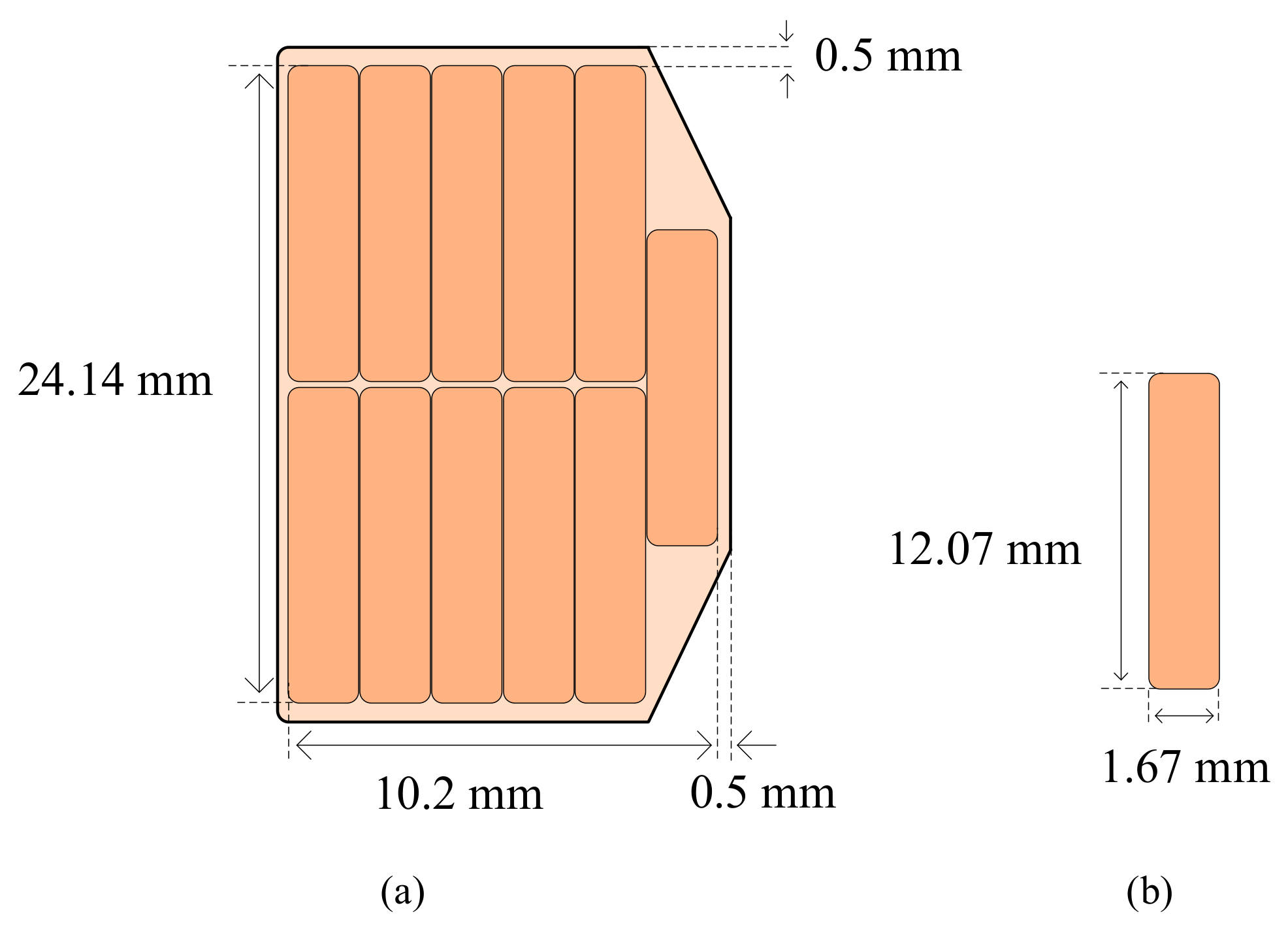
A turn is divided into several conductors arranged in parallel to reduce power losses due to eddy currents. The optimization process gives the number of conductors in one turn for LV winding 11 pieces. The arrangement of such conductors is two axially and six radially, shown in Figure 3. The optimization results show that the thickness of one conductor at a low-voltage winding is 1.67 mm, and the width of one conductor is 12.07 mm.
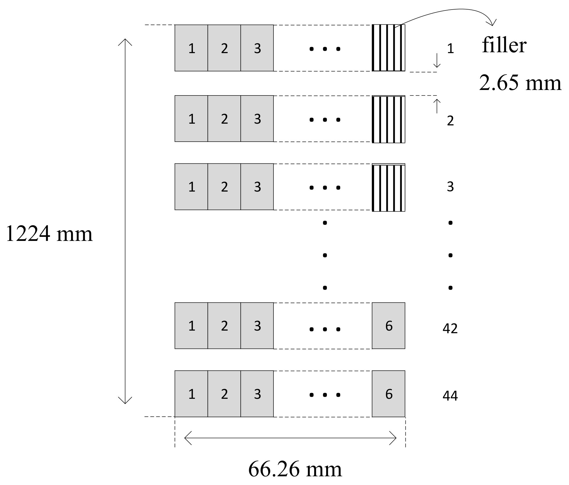
The optimization process gives the number of turns in one disk for LV winding six turns. According to (7), the width of the overall low voltage winding ( w LV ) is 66.26 mm. The number of disks for LV windings is the number of total turns of LV winding divided by the number of turns per disk. A total of 44 disks is obtained with a distance between disks of 2.65 mm. Only some disks contain six turns because the overall number of turns is 261, so there will be three disks containing five turns. The height of each disk is 25.14 mm, so based on (8), the height of the low-voltage winding is 1224 mm. The arrangement of low-voltage windings with 44 disks and six turns per disk is shown in Figure 4.
Based on (9), the phase current ( I HV ) for the high-voltage winding (star connecting) is 419.89 A. According to (10), the number of turns per phase of HV winding ( N HV 
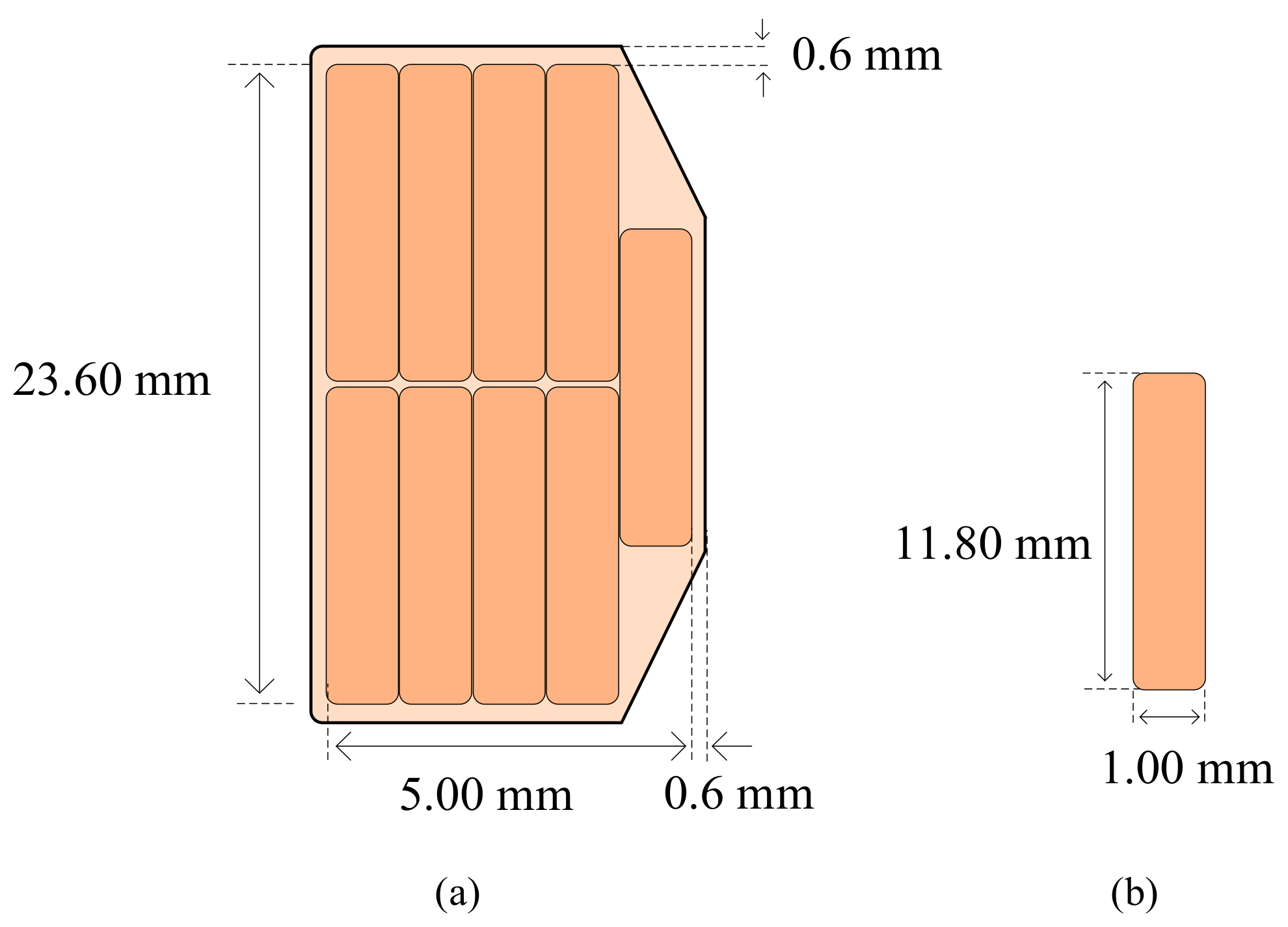
) is 503. The optimization process gives the number of conductors per turn in HV winding nine pieces, with two winding axially and five winding radially. The arrangement of the conductors and disk of HV winding is shown in Figure 5 and Figure 6. The dimensions of one conductor having a thickness of 1.00 mm and a width of 11.80 mm are indicated in Figure 5b. Based on (13), the overall width of HV winding ( w HV ) is 74.46 mm. According to (11), the cross-sectional area per turn at the HV winding ( A HV ) is 106.33 mm2. The current density (   δ HV ) of HV winding based on (12) is 3.95 A/mm2.
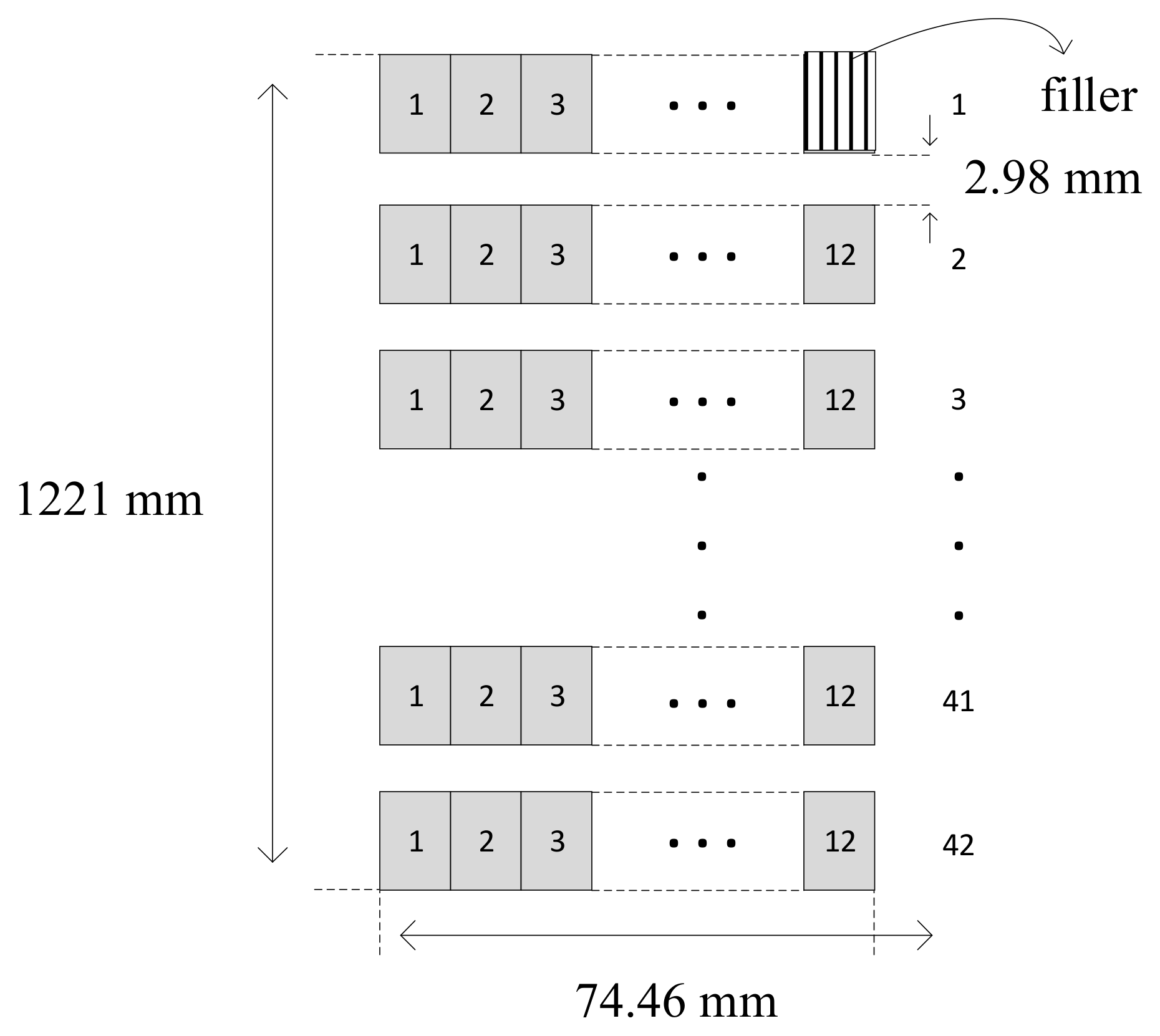
The optimization process gives the number of turns per disk for HV windings 12 turns. The number of disks of HV winding is the total turns of HV winding divided by the number of turns per disk, which makes the number of disks 42. Only some disks contain 12 turns because the overall number of turns is 503, so there will be one disk containing 11 turns. Therefore, to maintain its balance, a filler is needed. According to (14), the height of HV winding ( h HV ) is 1221 mm. The height of the HV winding is similar to that of the LV winding. The height similarity is to maintain magnetic balance in the winding.
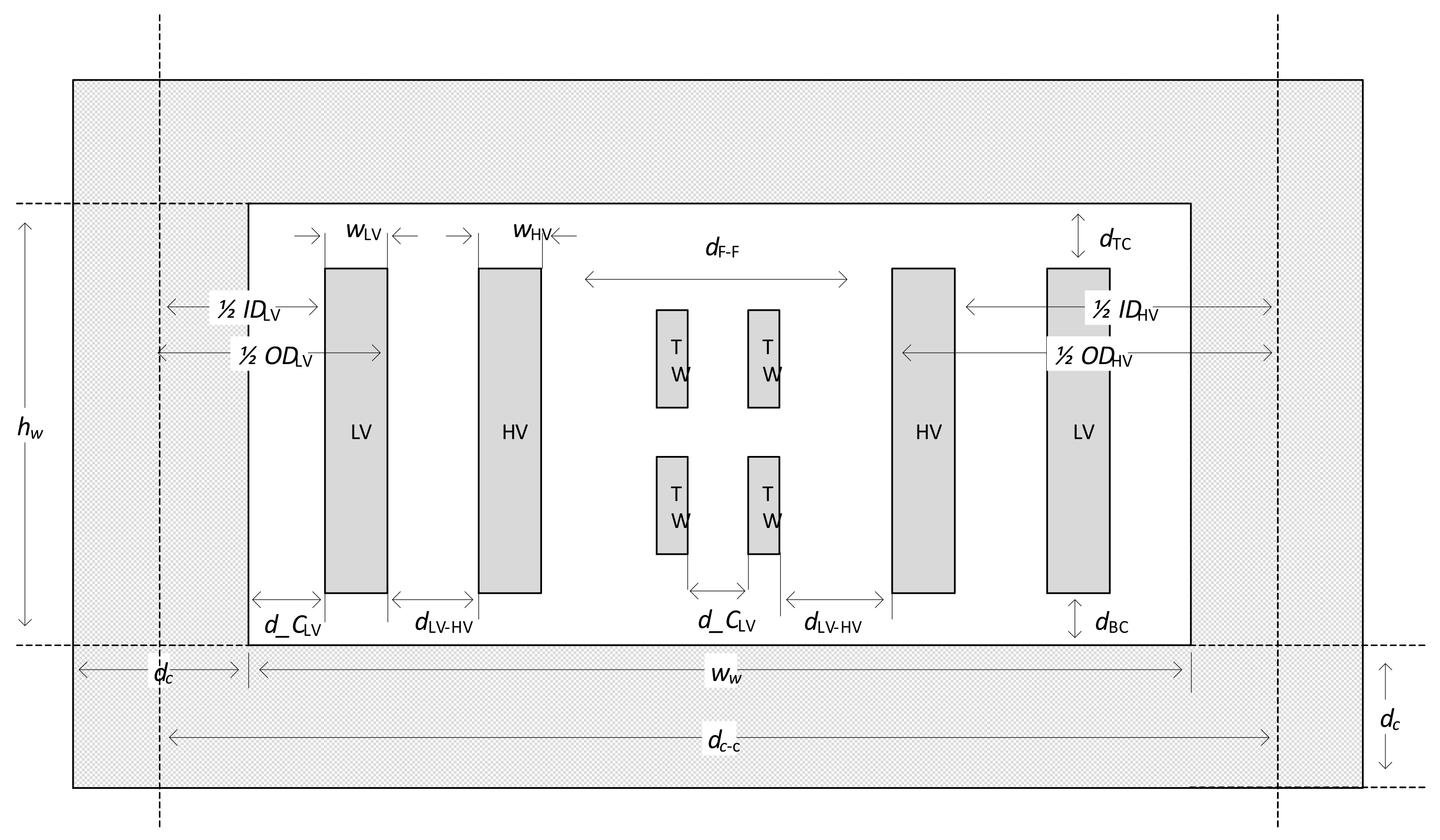
The winding and core dimensions for one window are shown in Figure 7. The diameter of the core ( d c ) and the diameter of the yoke are equally large at 626.4 mm. The tap winding (TW) is located separately from its primary winding and is placed in the middle between the HV windings for its phases. The distance between the HV windings and the tap windings equals the distance between the LV windings and the HV windings. At the same time, the distance between the tap windings is equal to the distance between the core and the LV windings. Table 5 is a summary of the core and winding dimensions.
The diameters of the limb and yoke are the same size, so based on (22), the total length of the core ( l C ) is 12,704.13 mm. This core length includes all the limbs and yoke of the top and bottom. Using the core weight per volume (   G c ) of 7650 kg/m3, then by (23) and (24), the total weight of the core ( W C ) is 36,993.10 kg.
The volume of the winding is calculated by taking the average diameter of each winding. Based on (25) and (26), the volumes of low-voltage and high-voltage windings are respectively 0.3906 m3 and 0.4738 m3. The weight per volume for the winding material (   G w ) is 8890 kg/m3, so the weight of the LV winding ( W LV ) and the HV winding ( W HV ) is 3472.21 kg and 4212.11 kg.
The LV winding resistance ( R LV ) and the HV winding resistance ( R HV ) were calculated using (37) and (38) so that the resistance of LV winding is 0.1669 Ω and HV winding is 0.8842 Ω, respectively. The total resistance of the transformer ( R ) based on its high voltage side can be derived by (39), obtaining 1.5040 Ω.
The dimensions of the winding strongly influence the impedance of the transformer. The impedance can be derived from (29) to (36). The cross-sectional area of the winding passed by the flux ( A ) is 0.2323 m2, and the Rogowski factor is 0.9597, then the leakage inductance based on the high voltage side ( L ) is 0.0579 H, and the leakage reactance of the transformer ( X ) is 18.20 Ω. The impedance of the power transformer is usually considered equal to the value per unit of its reactance. So ( X p u ) for this transformer when based on the side of high voltage is 12.04%. The impedance is still within the allowable limit range.
Copper losses are divided into two, namely copper losses on LV windings ( P L LV ) and HV windings ( P L HV ). In addition, there are losses due to eddy currents and stray losses. Based on (42) and (43), the copper losses in the LV and HV windings were 86.77 kW and 124.12 kW, respectively. Meanwhile, stray loss in structural components (frame and plate tank) is assumed to be 20% of the losses in the windings. So based on (49), the total load losses ( P L ) is 210.89 kW.
Two components dominate core losses ( P C ): eddy loss and hysteresis loss. For practical purposes, the value of the two losses is a multiplier factor ( K L ) between 1 and 1.25 of the core weight. The density loss at the core joint is higher than in other places. The equation assumes the weight at the core joint with a penalty factor ( K p ). By taking K L = 1 and K J = 0.3 , and K p = 1 , the core loss ( P C ) can be determined based on (41) as 36.99 kW. Based on (50) and (51) and considering all the losses obtained, the efficiency at full load and power factor unity is obtained by 99.56%. Based on (52) and (53), load noise ( L L ) and no-load noise ( L N L ) can be obtained by 69.33 and 69.32 dB. Total noise is a logarithmic aggregation of the three types of noise, so by excluding noise due to the cooling system, the noise coming from the core and winding is 71.3 dB.

4.2. Vibration and Noise Analysis with Finite Element Method

Accurate modeling of vibration and noise is highly dependent on the excellent coupling of magnetic, electrical, and mechanical domains [33]. This study modelled a three-phase power transformer with 80 MVA, three limbs, and double windings as a cylinder type. The core structure consists of four stages, and for simplicity, the power transformer tank is designed in the shape of a geometry box. The power transformer structure data obtained from the design optimization results using PSO are shown in Table 5 and Table 6.
Finite element mesh is applied for core and winding in the form of free tetrahedral with maximum element size 0.6 m, minimum size 0.108 m, maximum element growth rate 1.5, curvature factor 0.6, and resolution of narrow regions 0.5. The number of vertex elements is 284, the number of edge elements is 4757, the number of tetrahedra elements is 97,265, and the number of triangles elements is 25,697 with minimum element quality is 0.09535. According to [34], mesh size does not significantly affect the results but affects calculation time. The Figure 8 shows the finite element mesh for the designed power transformer.

4.2.1. Electromagnetic Field Analysis

The current flowing in the winding is assumed to be evenly distributed. The strength of the electromagnetic field will build up around the winding with varying values depending on the supply in the winding, the permeability of the core, air, and surrounding materials. Furthermore, the boundary is in the shape of a box that is used as magnetic shielding. The electromagnetic field is calculated by software simulation based on Maxwell’s Theory in Equations (69) to (71) as presented by [34].
J e = σ A t + × α 0 1 . α r 1   × A
B = α 0 α r = × A
J = σ E + J e
The magnetic field module based on Equations (69) to (71) is solved by setting the variables A x ,   A y , A z , and ψ . The maximum magnetic density for the core is 1.5 T. While the winding conductor is chosen as a circular coil type with a homogenized numeric multiturn coils model, with the conductivity of copper as 5.89 × 10⁷ S/m.

4.2.2. Structure Dynamics

The structural analysis deformation components u, v, and w are obtained by Equations (72) to (73). The coil domain is assumed to be a linear elastic material with the core as a magnetostrictive material
M σ = σ Ε ζ M o n M + c M o n σ
ϵ = 1 M Δ 2 + c Δ + K . A r Ε l r . ρ
The effective field in the core can be derived by Equation (74).
H e f f = H + 3 λ m α 0 η s 2 × M
The coefficient M describes the interaction of magnetism and stress. Meanwhile, the magnetization model can be defined by Equation (75).
ϑ = cot h 3 X m H e f f η s η s 3 X m H e f f
Some displacements as a result of simulation with COMSOL are shown in Figure 9. Each frequency gives different displacement results. The final resultant is the summation of all displacements to determine the deformation of the core.

4.2.3. Acoustics Analysis

Equations (76) to (77) are used to calculate the acoustics of the power transformer.
. 1 ρ c ρ t k e q 2 ρ c ρ t
k e q 2 = ω C c 2
where ρ 0 is the density of the fluid, p is the pressure, c is the speed of sound, ω is the angular frequency, and C c is the bulk modulus. The acoustics interface is used for acoustics studies. This interface is the result of coupled study with structural dynamics.

4.3. Numerical Design Validation

Numerical design validation of the power transformer is performed using COMSOL software. The 3D model illustration, including cores and windings, is shown in Figure 10. Based on data from Table 5 and Table 6. The parameters of relative conductivity, relative permeability, and relative magnetic permeability in the core are set to 1. A three-phase voltage source with 120° phase difference is connected to the HV winding, and the LV winding is assumed to flow nominal current for each phase.
Noise verification is performed by taking simulated data at several measurement points (MP). The measurement points are located at a distance of 0.3 m from the tank and at half the height of the transformer. The distance between measurement points is 0.5 m. The Table 7 shows the data taken from the simulation for 34 measurement points. Table 7 is the noise taken from several measurement points.
According to [35], the average of sound power level can be calculated by
L p A 0 ¯ = 10 log 10 1 N i = 1 N 10 0.1 L p A i
where L p A 0 ¯ is the average of sound power level, N is number of measurement point, and L p A i is the sound power level in the measurement point. According to (78), the average sound power level is 69.25 dB. Figure 11 illustrates the sound power distribution seen from top and side of power transformer.

4.4. Comparison of Design and Optimization

A comparison of design and optimization results is presented in Table 6. The optimization results provide a higher current density value than the design results. A higher current density will result in a smaller cross-sectional area for one turn, affecting the weight of the winding and its dimensions. The increase in current density is directly proportional to the decrease in winding material weight. The increase in current density in LV winding by 1.336 A/mm2 or 58% will reduce the weight of winding material by 2939.8 kg. While the increase in current density in HV winding by 1.6 A/mm2 or 68% will reduce the weight of HV winding material by 4.001 kg. However, another consideration is that with the current’s high density, the temperature increase will be higher, impacting the cooling system. The method to reduce the temperature rise is to add an extra radiator so that it does not impact the transformer noise. The winding height of the optimization result is lower than the design result and has a lower winding width. The core weight of the optimization results has a lower value than the design results, around 801.9 kg or a decrease of 2.12%. The winding weight of the optimization result is lighter than the design result, with a difference of 6941.68 kg or a decrease of 47.46%. These two parameters obtained significant savings, which will lower the cost of production. On the contrary, core losses and winding losses have increased compared to the design results. The primary cause of the increase in winding losses is the current density.
Based on (52), load noise is affected by the weight of the winding and the dimension ratio of the winding. Thus, with a decrease in winding weight and height, the optimization results provide a load noise value of 69.33 dB lower than the design results.
The objective function of this optimization is to minimize the weight of the core material, winding material, and load noise. The core’s material cost is cheaper than the material costs for its winding. For comparison, the price of winding material today is two times more expensive than that of the core material. Therefore, the optimization results provide a much cheaper material cost value while still getting a lower load noise. The optimization method with PSO can be used to design a low noise power transformer. The PSO method is beneficial in determining the optimal variables to produce a transformer design that meets the standards, is low-cost, and has low noise.

5. Conclusions

The paper introduced the optimization of low-load noise power transformer design. The PSO method can obtain optimum values of 11 variables that can be used to design low-load noise power transformers. The paper has set up a multi-objective function for optimal load noise, the weight of the core, and the weight of the winding. The optimization results showed a decrease in load noise, core weight, and winding weight by 0.86 dB, 2.12%, and 47.46%, respectively. The industry will benefit by applying this method, such as a low-noise power transformer design and obtaining economic benefits by optimizing the core and winding weight. The results of this optimization are better than the designs used regularly in the industry.

Author Contributions

Conceptualization, W.B.P., F.D.W., and S.P.H.; methodology, W.B.P., F.D.W., and S.P.H.; software, W.B.P.; validation, M.S.W., W.B.P., and A.I.; formal analysis, W.B.P., S.P.H., F.D.W., M.S.W., and A.I.; investigation, M.S.W. and A.I.; resources, M.S.W. and A.I.; data curation, M.S.W. and A.I.; writing—original draft preparation, W.B.P.; writing—review and editing, F.D.W. and S.P.H.; visualization, M.S.W., W.B.P., and A.I.; supervision, S.P.H.; project administration, W.B.P. and F.D.W.; funding acquisition, F.D.W. All authors have read and agreed to the published version of the manuscript.

Funding

This research was funded by the Final Project Recognition (RTA) program from Gadjah Mada University Yogyakarta, grant number 2448/UN1.P.III/DIT-LIT/PT/2020) and The APC was funded by The Islamic University of Indonesia (UII) Yogyakarta.

Data Availability Statement

Not applicable.

Acknowledgments

The authors are grateful for the following supporting data and financial support: PT Elsewedy Electric Indonesia and UII Yogyakarta. In addition, the author would like to thank PT PLN Indonesia for allowing the use of COMSOL software for model validation.

Conflicts of Interest

The authors declare no conflict of interest. The funders had no role in the design of the study; in the collection, analyses, or interpretation of data; in the writing of the manuscript; or in the decision to publish the results.

References

  1. Kennelly, R.J. IEEE Standards for Physical and Data Communications. Biomed. Instrum. Technol. 2002, 30, 172–175. [Google Scholar]
  2. Georgilakis, P.S. Spotlight on Modern Transformer Design; Springer: London, UK, 2009; ISBN 978-1-4471-2675-1. [Google Scholar]
  3. Del Vecchio, R.M.; Poulin, B.; Feghali, P.T.; Shah, D.M.; Ahuja, R. Transformer Design Principles: With Applications to Core-Form Power Transformers; CRC Press: Boca Raton, FL, USA, 2001; ISBN 9781420021943. [Google Scholar]
  4. Zhang, Z.; Xu, S.; Zhang, J.; Liu, H.; Huang, X.; Wang, Z.; Zhao, L. Study on Vibration Noise Signal Characteristics of 10kv Distribution Transformer under Different Load Conditions. In Proceedings of the Asia Conference on Power and Electrical Engineering, ACPEE 2019, Hangzhou, China, 28–31 March 2019; Volume 486, p. 012033. [Google Scholar]
  5. Kozupa, M.; Ploetner, C.; Swiatkowski, M. Acoustic Radiation Efficiency Parameter in Assessment of Transformer Noise. In Proceedings of the 11th European Congress and Exposition on Noise Control Engineering, Crete, Greece, 27–31 May 2018; pp. 573–578. [Google Scholar]
  6. Kepmen No: KEP-48/MENLH/11/1996 Tentang BAKU TINGKAT KEBISINGAN. Available online: https://ditppu.menlhk.go.id/portal/peraturan-nasional (accessed on 12 September 2019).
  7. Rohilla, V.; Palani Samy, C. A Study of Transformer Noise and Reduction Techniques of Transformer Noise. Trans. Korean Inst. Electr. Eng. 2017, 2, 1911–1915. [Google Scholar]
  8. Moses, A.J.; Anderson, P.I.; Phophongviwat, T. Localized Surface Vibration and Acoustic Noise Emitted from Laboratory-Scale Transformer Cores Assembled from Grain-Oriented Electrical Steel. IEEE Trans. Magn. 2016, 52, 1–15. [Google Scholar] [CrossRef]
  9. Gamil, A.; Schatzl, F. New Method to Optimize No-Load Noise of Power Transformers Based on Core Design & Transformer Operating Conditions. J. Energy 2014, 63, 43–51. [Google Scholar]
  10. Moses, A.J.; Anderson, I.; Phophongviwat, T.; Tabrizi, S. Contribution of Magnetostriction to Transformer Noise. In Proceedings of the 45th International Universities Power Engineering Conference UPEC2010, Cardiff, UK, 31 August 2010–3 September 2010. [Google Scholar]
  11. Vasques, C.M.A.; Miguel, H.; Campelo, R. Quiet Transformers: Design Issues. In Proceedings of the Advanced Research Workshop on Transformers, Baiona, Spain, 28–30 October 2013; pp. 1–17. [Google Scholar]
  12. Tanzer, T.; Pregartner, H.; Riedenbauer, M.; Labinsky, R.; Witlatschil, M.; Muetze, A.; Krischan, K. Magnetostriction of Electrical Steel and Its Relation to the No-Load Noise of Power Transformers. IEEE Trans. Ind. Appl. 2018, 54, 4306–4314. [Google Scholar] [CrossRef]
  13. Penin, R.; Lecointe, J.; Parent, G.; Brudny, J.; Belgrand, T. Estimation of Relative Magnetostriction and Maxwell’s Forces in Stacked Grain Oriented Steel Structures. In Proceedings of the 2012 XXth International Conference on Electrical Machines, Marseille, France, 2–5 September 2012; pp. 1971–1976. [Google Scholar]
  14. Case, J.J. Numerical Analysis of the Vibration and Acoustic Characteristics of Large Power Transformers; Queensland University of Technology Australia: Brisbane City, Australia, 2017. [Google Scholar]
  15. Amoiralis, E.I.; Tsili, M.A.; Paparigas, D.G.; Kladas, A.G. Global Transformer Design Optimization Using Deterministic and Nondeterministic Algorithms. IEEE Trans. Ind. Appl. 2014, 50, 383–394. [Google Scholar] [CrossRef]
  16. Olivares-Galvan, J.C.; Georgilakis, P.S.; Escarela-Perez, R.; Campero-Littlewood, E. Optimal Design of Single-Phase Shell-Type Distribution Transformers Based on a Multiple Design Method Validated by Measurements. Electr. Eng. 2011, 93, 237–246. [Google Scholar] [CrossRef]
  17. Tsili, M.; Amoiralis, E.I.; Leite, J.V.; Moreno, S.R.; Coelho, L.d.S. A Novel Multiobjective Lognormal-Beta Differential Evolution Approach for the Transformer Design Optimization. Eng. Comput. 2018, 35, 955–978. [Google Scholar] [CrossRef]
  18. Kulkarni, S.; Khaparde, S.A. Transformer Engineering, 2nd ed.; CRC Press: Boca Raton, FL, USA, 2017; ISBN 9781315217338. [Google Scholar]
  19. Mehta, H.D.; Patel, R.M. A Review on Transformer Design Optimization and Performance Analysis Using Artificial Intelligence Techniques. Int. J. Sci. Res. 2014, 3, 726–733. [Google Scholar]
  20. Weiser, B.; Pfützner, H.; Anger, J. Relevance of Magnetostriction and Forces for the Generation of Audible Noise of Transformer Cores; IEEE: New York, NY, USA, 2000; Volume 36. [Google Scholar]
  21. Rens, J.; Jacobs, S.; Van Poucke, M.; Attrazic, E. Numerical and Experimental Evaluation of Magnetostriction and Magnetic Forces on Transformer Stacks and Joints for the Assessment of Core Vibrations. In Proceedings of the 2017 IEEE Energy Conversion Congress and Exposition (ECCE), Cincinnati, OH, USA, 1–5 October 2017; Volume 2017, pp. 3111–3118. [Google Scholar]
  22. Azuma, D.; Hasegawa, R. Audible Noise from Amorphous Metal and Silicon Steel-Based Transformer Core. In Proceedings of the IEEE Transactions on Magnetics; IEEE: New York, NY, USA, 2008; Volume 44, pp. 4104–4106. [Google Scholar]
  23. Zhang, L.; Zhang, D.; Shui, H.; Yuan, Y.; Pei, Q.; Zhu, J. Optimisation Design of Medium Frequency Transformer for the Offshore Dc Grid Based on Multi-Objective Genetic Algorithm. IET Power Electron. 2017, 10, 2157–2162. [Google Scholar] [CrossRef]
  24. Eseosa, O. A Review of Intelligent Based Optimization Techniques in Power. Appl. Res. J. 2015, 1, 78–88. [Google Scholar]
  25. Andersen, W. Optimized Design of Electric Power Equipment. IEEE Comput. Appl. Power 1991, 4, 11–15. [Google Scholar] [CrossRef] [PubMed]
  26. Wu, C.; Lee, F.; Davis, R. Minimum Weight EI Core and Pot Core Inductor and Transformer Designs. IEEE Trans. Magn. 1980, 16, 755–757. [Google Scholar] [CrossRef]
  27. Doulamis, N.D.; Doulamis, A.D.; Georgilakis, P.S.; Kollias, S.D.; Hatziargyriou, N.D. A Synergetic Neural Network-Genetic Scheme for Optimal Transformer Construction. Integr. Comput. Aided. Eng. 2002, 9, 37–56. [Google Scholar] [CrossRef]
  28. Paghadar, H.; Kantaria, R.A. Accurate Estimation and Mitigation of Audible Sound Using Novel Technique of Flux Density Reduction at Design Stage in Transformer. Int. J. Electr. Electron. Eng. 2016, 3, 12–15. [Google Scholar] [CrossRef]
  29. Reiplinger, E. Study of Noise Emitted by Power Transformers Based on Todays Viewpoint.Pdf. In Proceedings of the International Conference on Large High Voltage Electric Systems; CIGRE: Paris, France, 1988; pp. 1–7. [Google Scholar]
  30. Pramono, W.B.; Wijaya, F.D.; Hadi, S.P.; Wahyudi, M.S.; Indarto, A. Power Transformer Load Noise Model Based on Backpropagation Neural Network. IJTECH 2022, Submitted. [Google Scholar]
  31. Pramono, W.B.; Wijaya, F.D.; Hadi, S.P. Prediction Formula Development of Power Transformer No-Load Noise. J. Phys. Conf. Ser. 2021, 1858, 012014. [Google Scholar] [CrossRef]
  32. Parsopoulos, K.E.; Vrahatis, M.N. Particle Swarm Optimization and Intelligence: Advances and Applications; Information Science Reference; IGI Global: Hershey, PA, USA, 2010; ISBN 9781615206667. [Google Scholar]
  33. Karafi, M.R.; Nejabat, R.S. An Introduction to a Bulk Magnetostrictive Bending Actuator Using a Permendur Rod. SN Appl. Sci. 2020, 2, 1–10. [Google Scholar] [CrossRef]
  34. Yadav, S.; Mehta, R.K. Modelling of Magnetostrictive Vibration and Acoustics in Converter Transformer. IET Electr. Power Appl. 2021, 15, 332–347. [Google Scholar] [CrossRef]
  35. Doğan, E.; Kekezoğlu, B. Power Transformer Noise, Noise Tests, and Example Test Results. World Acad. Sci. Eng. Technol. Int. J. Electr. Comput. Energ. Electron. Commun. Eng. 2016, 10, 57–61. [Google Scholar]
Figure 1. The flowchart of the PSO model.
Designs 07 00031 g001
Figure 2. The optimization results.
Designs 07 00031 g002
Figure 3. (a) The dimension and the arrangement of one turn and (b) the dimension of one conductor for LV winding.
Designs 07 00031 g003
Figure 4. The arrangement of disk for LV winding.
Designs 07 00031 g004
Figure 5. (a) The dimension and the arrangement of one turn, and (b) the dimension of one conductor for HV winding.
Designs 07 00031 g005
Figure 6. The arrangement of disk for HV winding.
Designs 07 00031 g006
Figure 7. Dimension of the core and the winding in one window.
Designs 07 00031 g007
Figure 8. Developed mesh.
Designs 07 00031 g008
Figure 9. Vibration displacement with varying frequency.
Designs 07 00031 g009aDesigns 07 00031 g009b
Figure 10. The 3D model of power transformer.
Designs 07 00031 g010
Figure 11. Sound power level distribution viewed from (a) top and (b) side.
Designs 07 00031 g011
Table 1. The lower and upper bounds of the optimized design variables.
VariableLower BoundUpper BoundUnit
w LV 1 13mm
n _ R LV 16conductor
n _ A LV 12conductor
n _ L D LV 612turn
w HV 1 13mm
  δ LV 34A/mm2
n _ R HV 16conductor
n _ A HV 12conductor
n _ L D HV 612turn
B m 1.41.7T
K t 0.40.7-
Table 2. The power transformer specifications.
ParameterSymbolValueUnit
Power( S )80MVA
Frequency( f )50Hz
Voltage of HV side( V HV )110kV
Voltage of LV side( V LV )33kV
Limbs 3-
Phase 3-
Impedance( Z )12%
Table 3. The PSO parameters.
ParameterValue
Number of particles250
Number of optimized variables11
Number of the maximum iteration25
Cognitive parameter2
Social parameter4
Table 4. The result of optimized variables.
VariableValueUnit
w LV 1 1.67(mm)
n _ R LV 6cond.
n _ A LV 2cond.
n _ L D LV 6Turn
w HV 1 1.00(mm)
  δ LV 3.636A/mm2
n _ R HV 5cond.
n _ A HV 2cond.
n _ L D HV 12turn
B m 1.496T
K t 0.4471
Table 5. Dimension of the core and the winding.
VariableSymbolValue (mm)
Diameter of the core d c 626.4
Distance between core and LV winding d _ C LV 10.77
Width of LV winding w LV 66.26
Inner diameter of LV winding I D LV 647.96
Outer diameter of LV winding O D LV 780.47
Distance between LV and HV winding d LV HV 42.31
Width of HV winding w HV 74.46
Inner diameter of HV winding I D HV 865.09
Outer diameter of HV winding O D HV 1014.02
Distance between center of limb d C C 1779.82
Distance between HV winding d F F 139.37
Distance between top winding and yoke d TC 110
Distance between bottom winding and yoke d BC 110
Height of the window h w 1444
Width of the window w w 1153.4
Table 6. Comparison of the results of design and optimization parameters with PSO.
ParameterSymbolResultsUnit
DesignPSO
PowerS80MVA
Frequencyf50Hz
HV side voltage V HV 110kV
LV side voltage V LV 33kV
Number of limbs 3
Phase 3
Nominal current of LV winding I LV 808.1808.1A
Nominal current of HV winding I HV 419.6419.6A
ImpedanceZpu1212.04%
Number of LV windings N LV 243261turn
Number of HV windings N HV 468503turn
LV winding height h LV 15871224mm
High winding HV h HV 15531221mm
LV winding width w LV 9366.26mm
HV winding width w HV 9574.46mm
Outer diameter of LV winding O D LV 966780.47mm
Outer diameter of HV winding O D HV 12361014.02mm
LV winding weight W LV 64123472.21kg
HV winding weight W HV 82144212.11kg
LV current density   δ LV 2.33.636A/mm2
HV current density   δ HV 2.353.95A/mm2
Magnetic flux density B m 1.5621.496T
Core weight W C 37,79536,993.10kg
Core cross-sectional area A c 39143806.4mm3
Core losses P C 28.536.99kW
Winding losses P L 198.5210.89kW
Load noise L L 70.1969.33dB
No load noise L N L 69.5769.32dB
Table 7. Noise data from measurement points.
MPNoise (dB)MPNoise (dB)
173.931866.29
273.381963.57
371.822061.45
469.332173.40
566.222271.87
663.772369.47
761.592466.42
873.332563.69
971.792661.59
1069.212762.49
1166.252863.16
1263.512963.15
1361.453062.47
1473.893162.49
1573.363263.17
1671.813363.15
1769.363462.57
Disclaimer/Publisher’s Note: The statements, opinions and data contained in all publications are solely those of the individual author(s) and contributor(s) and not of MDPI and/or the editor(s). MDPI and/or the editor(s) disclaim responsibility for any injury to people or property resulting from any ideas, methods, instructions or products referred to in the content.

