
Secured Multi-Dimensional Robust Optimization Model for Remotely Piloted Aircraft System (RPAS) Delivery Network Based on the SORA Standard


Abstract
:1. Introduction
- -
- the RPAS-based distribution network of a supply chain was implemented at three echelons: facility locations, DCs, and demand points, while in other studies, path planning was not examined in more than two echelons.
- -
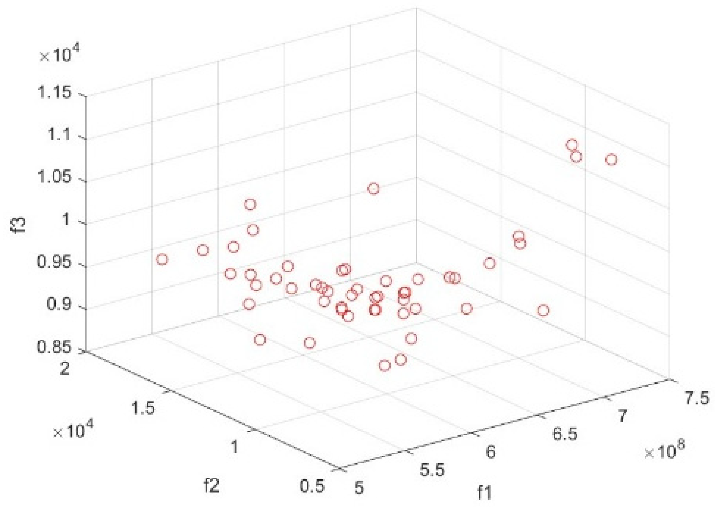
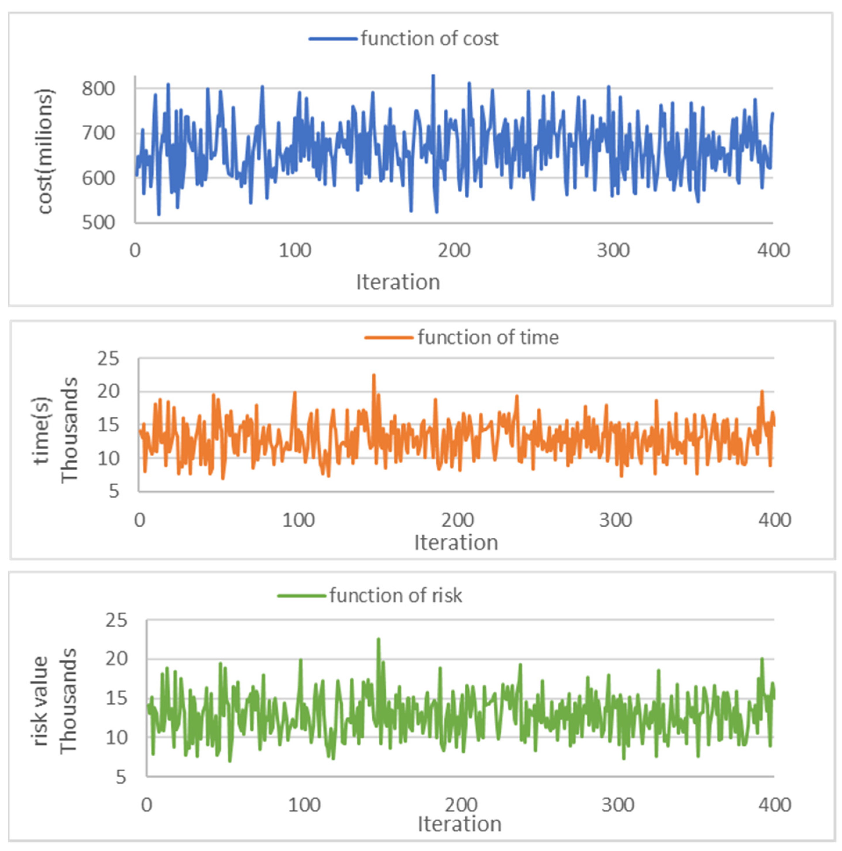
- Optimization was carried out aiming to reduce three significant factors simultaneously in the model: cost, delivery time, and imposed risk. They were modeled to be minimized as the first, second, and third objective functions, respectively.
- -
- Contrary to previous studies, constraints related to the demand, delivery time, and battery usage variables were considered simultaneously to make the model close to the real state of a distribution system.
- -
- In the second part of the objective function in the proposed model based on different traffic scenarios, the data on the time of delivery were considered uncertain, which aims at finding answers close to optimized. Among the matters proposed to regulate uncertain data, we deployed Malloy’s robust optimization model.
- -
- In this study, the identified risks in each graph were developed in the form of a model and minimized as the third objective. For the first time, the risk assessment approach was conducted based on the SORA standard.
- -
- In the level of distribution DCs, they were located along with RPAS routing planning.
- -
- A novel NSGA-II algorithm was justified specifically for the introduced model.
2. Literature Review
2.1. Drone Routing Problem Considering Time, Demand, and Battery Constraints
2.2. Robust Optimization in RPA Delivery Model
2.3. Risk Assessment Model for RPA Delivery Model
3. Methodology
3.1. Objective Function
3.1.1. The Function of Cost
3.1.2. The Function of Time
3.1.3. The Function of Risk
- Identifying and weighing efficacious risk indicators for the path (assessed by the SORA approach).
- Employing average to specify the weights of each facture.
- Calculating the risk of each route by applying the weights ( assigned to the route risk variables through the equation .
- Designing a risk matrix for the pathways from node i to node j.
- The third goal’s function is to choose the route with the minimum risk via our proposed model.
- Ground risk elements
- Air risk elements
3.1.4. Mathematical Model
3.1.5. Assumptions
- -
- The drones make one-to-many delivery trips at the first echelon (from the facility location to the DCs) and many-to-many trips at the second echelon (from DCs to demand points and back) until the battery needs to be re-charged. It includes a minimum energy also set for emergencies.
- -
- We do not consider one-to-many vehicle routing type trips, which are consistent with the initial applications of RPA deliveries by private companies.
- -
- We also do not consider battery recharging during the planning period for DCs where recharging is not possible and assume that the RPA battery is recharged between planning periods, but for those where it is possible, the service time at each site includes refueling time (time to recharge the RPA’s battery), if needed.
- -
- The length of the planning period is shorter (6 h to a day or 2 days) compared with the planning period for a typical facility location problem.
- -
- Another important assumption for the development of the mathematical model is related to the first m actions. They are dummy event locations used to represent the RPAS’s initial positions. Thus, no time windows are associated with these events, but they are simply born at the scenario starting time instant and remain active for all durations of the scenario itself.
- -
- We refer to the RPA as any aircraft capable of moving autonomously at varied and heterogeneous velocity, capacity, battery consumption, and purchasing cost.
- -
- Each RPA can serve more than one demand point per dispatch as long as its flight range and load carrying capacity are not violated.
- -
- RPAs can return to the same DCs along the route.
- -
- Multiple RPAs can be dispatched simultaneously from any DCs, which allows the use of a swarm of RPAs to enhance the overall productivity of the system.
- -
- We assume that applied RPAs have the battery capacity to cover the longest planning period, and before per dispatch, operators ensure that drones have enough battery to the end of the route.
- -
- There are limited DCs equipped with recharging stations
- -
- Customers are served only by RPAs.
- -
- RPAs can be dispatched and collected several times from the same DCs.
- -
- RPA batteries are replaced with fully charged batteries each time.
- -
- Packages are loaded and unloaded from the RPAs once the RPAs deliver to DCs or demand points.
- -
- After battery replacement and package loading/unloading, the RPA can be dispatched again to serve a new set of demand points. The process is repeated until all demand points in the service area have been reached.
4. Solution Representation
4.1. Non-Dominated Arranging Genetic Algorithm II NSGA-II’s Construction
- -
- Solution x is not worse than another solution y for any of the goal’s functions.
- -
- x is strictly superior to y in at least one of the n goal’s functions. This procedure will be repeated until all non-dominant solutions have been eliminated.
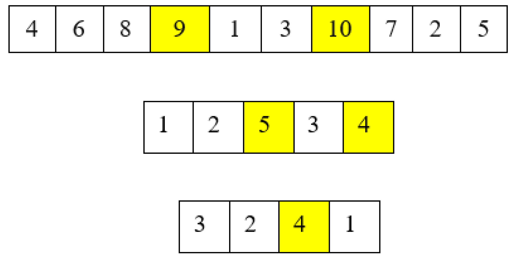
4.1.1. Initial Population
4.1.2. Parents Selection
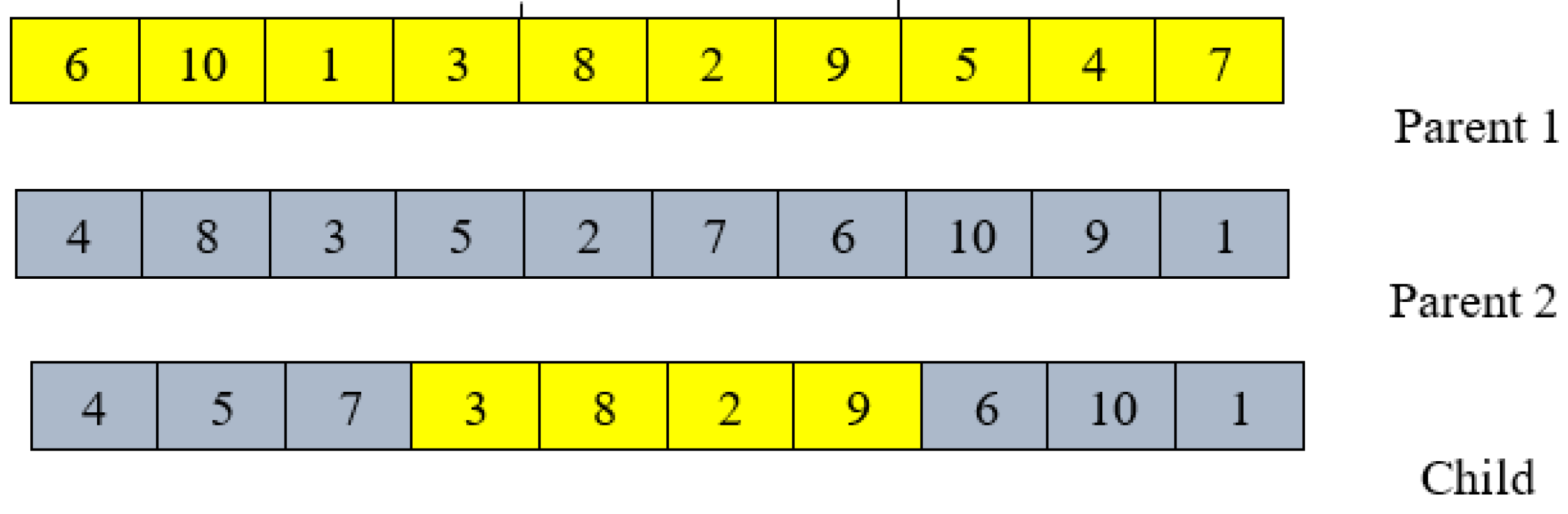
4.1.3. The Crossover Operator to Produce New Children
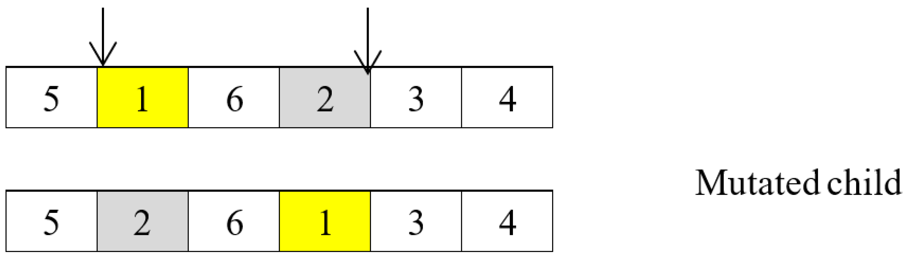
4.1.4. Mutation Operator
5. Computational Result
5.1. Input Data for NSGA-II Parameters
5.2. Input Data for Risk Model Parameters
- -
- The RPA has a technical issue (OSO # 1-OSO # 10);
- -
- External systems that support RPA functioning are deteriorating. (OSO # 11-OSO # 13);
- -
- Errors made by individuals (OSO # 14-OSO # 20);
- -
- Unpleasant performing conditions (OSO # 21-OSO # 24) [48].
- Selected RPA: Arm pitch 83 cm hexa-rotor, Maximum Take-off Weight (MTOW) m = 12 kg, cruise speed v = 8 m/s.
- Population: n/SS = high populated (10,000 n/m2 or 3853 n/km2).
- Arm pitch 0.83 × 0.83 m from a hexa-rotor.
- Kinetic energy of RPA (KE): 384 Joules, from a hexa-rotor.
- MTOW (m): 12 kg.
- Velocity (v): 8 m/s (maximum operating speed of hexa-rotor H83)
5.3. AHP Ranking Method
- Create an enforced routing risk matrix, S =, with m = n representing the number of risk criteria. The criteria are based on the SORA approach and contain elements that influence the occurrence of events that cause an incident.
- Experts provide a numerical scale to each pairing of n criteria (Si, Sj) at the first level of hierarchy.
- 3.
- Once all the experts express their judgement, the geometric mean of their values are computed as follows:The acquired Sij is then placed as its input into the matrix D:
- 4.
- At this stage, the weights of the criteria are computed by summing the columns of the normalized Matrix W, which, as said by Saati [59], is a comparison matrix with the following attributes.
- 5.
- In the final matrix , rank the criteria in decreasing order of the computed values; the inputs of are used as the value of in Equation (39).
6. Results and Discussion
Parameters Analysis
7. Conclusions
Author Contributions
Funding
Institutional Review Board Statement
Informed Consent Statement
Data Availability Statement
Conflicts of Interest
Abbreviations
| RPAS | Remotely Piloted Aircraft System |
| SORA | Specific Operation Risk Assessment |
| ICT | Information and Communications Technology |
| DC | Distribution Center |
| IOT | Internet of Things |
| FAA | Federal Aviation Administration |
| EASA | European Aviation Safety Agency |
| MLRP | Multi-objective Location-Routing Problem |
| NAS | National Aviation System |
| MCDM | Multi Criteria Decision Making |
| LRPD | Location-Routing problem with Drones |
| ARC | Air risk class |
| GRC | Ground risk class |
| MTOW | Maximum Take-off Weight |
| OSO | Operational safety objectives |
| NPOP | Number of Population |
| NSGA-II | Non-dominated sorting genetic algorithm II |
Appendix A
- sets
| Decision Variables | |
| D: | A set of distributor candidate locations |
| F: | A set of facility locations |
| P: | A set of demand points |
| K: | A set of drones |
| D1: | A set of demand points where recharging is possible |
| D2: | A set of demand points where recharging is not possible |
| U: | A set of different scenarios |
- Parameters
| Parameters | Description |
| ri: | The amount of delivery demand of demand points i |
| Pi: | The amount of pickup demand of demand points i |
| Si: | Time to provide service to demand points i |
| : | Loading capacity of each RPA k |
| ai: | The earliest time allowed to provide service to distributor i in the hard time window |
| bi: | The latest time allowed to provide service to distributor i in the hard time window |
| M: | Optional large number |
| ESi: | The earliest time allowed to provide service to distributor i in the soft time window |
| LSi: | The latest time allowed to provide service to distributor i in the soft time window |
| W2: | Cost per unit time deviation from the earliest time allowed in the soft time window |
| W3: | Cost per unit time deviation from the latest time allowed in the soft time window |
| : | Fixed cost of using RPA k |
| : | Cost of one charging unit |
| : | Minimum amount of charging allowed inside the RPA |
| : | Preparing cost of a unit in facility location f |
| : | Cost of constructing distributor candidate location d |
| : | Time to provide service to demand point i |
| DAY: | The length of a working day |
| : | RPA battery consumption from node i to node j |
| dxij: | The distance between node i and node j |
| : | Battery charging capacity |
| : | The probability of occurrence of scenarios u |
| : | The velocity of RPA k in event u |
| : | The capacity of candidate location of distributor d |
| : | The capacity of facility location f |
| L0k: | The load on RPA k when leaving the distributor |
| The risk of route deriving from node i to node j with RPA k | |
| : | belonging to candidate distributor locations d travels from node i to node j, it is equal to one and otherwise zero |
| : | The time to start providing service to demand point i in scenario u |
| Lj: | The weight of the load remaining on the RPA after service to demand point j |
| The variables zero and one. If distributor d is constructed, it is equal to one and otherwise zero | |
| : | The time deviation from the earliest time allowed to provide service to demand point i in the soft time window in scenario u |
| : | The time deviation from the latest time allowed to provide service to demand point i in the soft time window in scenario u |
| The time to end the route of RPA k | |
| The center demand of distributor d | |
| Variables zero and one. If distributor d is assigned to facility location f, it is equal to one and otherwise zero | |
| : | The amount of battery available on the RPA |
References
- Joerss, M.; Schroder, J.; Neuhaus, F.; Klink, C.; Mann, F. Parcel Delivery: The Future of Last Mile; Mckinsey & Company: London, UK, 2016. [Google Scholar]
- Karak, A.; Abdelghany, K. The hybrid vehicle-drone routing problem for pick-up and delivery services. Transp. Res. Part C 2019, 102, 427–449. [Google Scholar] [CrossRef]
- Peng, K.; Liu, W.; Sun, Q.; Ma, X.; Hu, M.; Wang, D.; Liu, J. Wide-Area Vehicle-Drone Cooperative Sensing: Opportunities and Approaches. IEEE Access 2019, 7, 1818–1828. [Google Scholar] [CrossRef]
- Dawaliby, S.; Aberkane, A.; Bradai, A. Blockchain-based IoT platform for autonomous drone operations management. In Proceedings of the 2nd ACM MobiCom Workshop on Drone Assisted Wireless Communications for 5G and Beyond, London, UK, 25 September 2020. [Google Scholar]
- Xiang, G.; Hardy, A.; Rajeh, M.; Venuthurupalli, L. Design of the life-ring drone delivery system for rip current rescue. In Proceedings of the 2016 IEEE Systems and Information Engineering Design Symposium (SIEDS), Charlottesville, VA, USA, 29 April 2016; pp. 181–186. [Google Scholar]
- Albornoz, C.; Giraldo, L.F. Trajectory design for efficient crop irrigation with a UAV. In Proceedings of the 2017 IEEE 3rd Colombian Conference on Automatic Control (CCAC), Cartagena, Colombia, 18–20 October 2017; pp. 1–6. [Google Scholar]
- Troudi, A.; Addouche, S.-A.; Dellagi, S.; El Mhamedi, A. Logistics Support Approach for Drone Delivery Fleet. In Proceedings of the 14th International Conference on Smart Cities, Málaga, Spain, 11–12 November 2017; pp. 86–96. [Google Scholar] [CrossRef]
- Kunze, O. Replicators, Ground Drones and Crowd Logistics A Vision of Urban Logistics in the Year 2030. Transp. Res. Procedia 2016, 19, 286–299. [Google Scholar] [CrossRef]
- Menouar, H.; Guvenc, I.; Akkaya, K.; Uluagac, A.S.; Kadri, A.; Tuncer, A. UAV-enabled intelligent transportation systems for the smart city: Applications and challenges. IEEE Commun. Mag. 2017, 55, 22–28. [Google Scholar] [CrossRef]
- Dehin, G.; Zanetti, M.; de Araújo, O.; Cardoso, G., Jr. Minimizing dispersion in multiple drone routing, Computer and operation research. Comput. Oper. Res. 2019, 109, 28–42. [Google Scholar] [CrossRef]
- Alfeo Mario, A.L.; Cimino, G.C.A.; Vaglini, G. Enhancing biologically inspired swarm behavior: Metaheuristics to foster the optimization of UAVs coordination in target search. Comput. Oper. Res. 2019, 110, 34–47. [Google Scholar] [CrossRef]
- Hu, X.; Pang, B.; Dai, F.; Low, K.H. Risk Assessment Model for UAV Cost-Effective Path Planning in Urban Environments. IEEE Access 2020, 8, 150162–150173. [Google Scholar] [CrossRef]
- Guerriero, F.; Surace, R.; Loscrí, V.; Natalizio, E.A. Multi-objective approach for unmanned aerial vehicle routing problem with soft time windows constraints. Appl. Math. Model. 2014, 38, 839–852. [Google Scholar] [CrossRef]
- Doole, M.; Ellerbroek, J.; Hoekstra, J. Estimation of traffic density from drone-based delivery in very low level urban airspace. J. Air Transp. Manag. 2020, 88, 101862. [Google Scholar] [CrossRef]
- Janik, P.; Zawistowski, M.; Fellner, R.; Zawistowski, G. Unmanned Aircraft Systems Risk Assessment Based on SORA for First Responders and Disaster Management. Appl. Sci. 2021, 11, 5364. [Google Scholar] [CrossRef]
- Chauhan, D.R.; Unnikrishnan, A.; Figliozzi, M.; Boyles, S.D. Robust Maximum Coverage Facility Location Problem with Drones Considering Uncertainties in Battery Availability and Consumption. Transp. Res. Rec. 2021, 2675, 25–39. [Google Scholar] [CrossRef]
- Chauhan, D.; Unnikrishnan, A.; Figliozzi, M. Maximum Coverage Capacitated Facility Location Problem with Range Constrained Drones. Transp. Res. Part C Emerg. Technol. 2019, 99, 1–18. [Google Scholar] [CrossRef]
- Park, H.; Son, D.; Koo, B.; Jeong, B. Waiting strategy for the vehicle routing problem with simultaneous pickup and delivery using genetic algorithm. Expert Syst. Appl. 2020, 165, 113959. [Google Scholar] [CrossRef]
- Ohmori, S.; Yoshimoto, K. Multi-product multi-vehicle inventory routing problem with vehicle compatibility and site dependency: A case study in the restaurant chain industry. Uncertain Supply Chain Manag. 2021, 9, 351–362. [Google Scholar] [CrossRef]
- Khoufi, I.; Laouiti, A.; Adjih, C.; Hadded, M. UAVs Trajectory Optimization for Data Pick Up and Delivery with Time Window. Drones 2021, 5, 27. [Google Scholar] [CrossRef]
- Choi, Y.; Schonfeld, P.M. Drone Deliveries Optimization with Battery Energy Constraints. In Proceedings of the Transportation Research Board 97th Annual Meeting, Washington, DC, USA, 7–11 January 2018. [Google Scholar]
- Allouch, A.; Koubaa, A.; Khalgui, M.; Abbes, T. Qualitative and Quantitative Risk Analysis and Safety Assessment of Unmanned Aerial Vehicles Missions Over the Internet. IEEE Access 2019, 7, 53392–53410. [Google Scholar] [CrossRef]
- Wang, S.; Na, J.; Xing, Y. Adaptive optimal parameter estimation and control of servo mechanisms: Theory and experiments. IEEE Trans. Ind. Electron. 2020, 68, 598–608. [Google Scholar] [CrossRef]
- Sanz, D.; Valente, J.; del Cerro, J.; Colorado, J.; Barrientos, A. Safe operation of mini UAVs: A review of regulation and best practices. Adv. Robot. 2015, 29, 1221–1233. [Google Scholar] [CrossRef] [Green Version]
- Wu, G.; Zhao, K.; Cheng, J.; Ma, M. A Coordinated Vehicle–Drone Arc Routing Approach Based on Improved Adaptive Large Neighborhood Search. Sensors 2022, 22, 3702. [Google Scholar] [CrossRef]
- Barmpounakis, E.N.; Vlahogianni, E.I.; Golias, J.C. Unmanned Aerial Aircraft Systems for transportation engineering: Current practice and future challenges. Int. J. Transp. Sci. Technol. 2016, 5, 111–122. [Google Scholar] [CrossRef]
- Marinelli, M.; Caggiani, L.; Ottomanelli, M.; Dell’Orco, M. En route truck–drone parcel delivery for optimal vehicle routing strategies. IET Intell. Transp. Syst. 2018, 12, 253–261. [Google Scholar] [CrossRef]
- Coutinho, W.P.; Battarra, M.; Fliege, J. The unmanned aerial vehicle routing and trajectory optimization problem, a taxonomic review. Comput. Ind. Eng. 2018, 120, 116–128. [Google Scholar] [CrossRef] [Green Version]
- Cheng, C.; Adulyasak, Y.; Rousseau, L.M.; Sim, M. Robust Drone Delivery with Weather Information, optimization online, internet database. History 2019, 1–37. Available online: www.optimization-online.org/DB_FILE/2020/07/7897.pdf (accessed on 15 April 2022).
- Rojas Viloria, D.; Solano-Charris, E.L.; Muñoz-Villamizar, A.; Montoya-Torres, J.R. Unmanned aerial vehicles/drones in vehicle routing problems: A literature review. Int. Trans. Oper. Res. 2021, 28, 1626–1657. [Google Scholar] [CrossRef]
- Macrina, G.; Di Puglia Pugliese, L.; Guerriero, F.; Laporte, G. Drone-aided routing: A literature review. Transp. Res. Part C Emerg. Technol. 2020, 120, 102762. [Google Scholar] [CrossRef]
- Poikonen, S.; Campbell, J.F. Future directions in drone routing research. Networks 2021, 77, 116–126. [Google Scholar] [CrossRef]
- Kitjacharoenchai, P.; Min, B.; Lee, S. Two echelon vehicle routing problem with drones in last mile delivery. Int. J. Prod. Econ. 2020, 225, 107598. [Google Scholar] [CrossRef]
- Kuo, R.; Lu, S.-H.; Lai, P.-Y.; Mara, S.T.W. Vehicle routing problem with drones considering time windows. Expert Syst. Appl. 2022, 191, 116264. [Google Scholar] [CrossRef]
- Ribeiro, R.G.; Junior, J.R.C.; Cota, L.P.; Euzebio, T.A.M.; Guimaraes, F.G. Unmanned Aerial Vehicle Location Routing Problem with Charging Stations for Belt Conveyor Inspection System in the Mining Industry. IEEE Trans. Intell. Transp. Syst. 2020, 21, 4186–4195. [Google Scholar] [CrossRef]
- Lin, X.; Wang, C.; Wang, K.; Li, M.; Yu, X. Trajectory planning for unmanned aerial vehicles in complicated urban environments: A control network approach. Transp. Res. Part C Emerg. Technol. 2021, 128, 103120. [Google Scholar] [CrossRef]
- Gunawardena, N.; Leang, K.K.; Pardyjak, E. Particle swarm optimization for source localization in realistic complex urban environments. Atmos. Environ. 2021, 262, 118636. [Google Scholar] [CrossRef]
- Lynskey, J.; Thar, K.; Oo, T.Z.; Hong, C.S. Facility Location Problem Approach for Distributed Drones. Symmetry 2019, 11, 118. [Google Scholar] [CrossRef] [Green Version]
- Faiz, T.I.; Vogiatzis, C.; Noor-E-Alam, M. Robust Two-Echelon Vehicle and Drone Routing for Post Disaster Humanitarian Operations. arXiv 2020, arXiv:2001.06456. [Google Scholar]
- Shahzaad, B.; Bouguettaya, A.; Mistry, S. Robust Composition of Drone Delivery Services under Uncertainty. In Proceedings of the 2021 IEEE International Conference on Web Services (ICWS), Chicago, IL, USA, 5–10 September 2021; pp. 675–680. [Google Scholar]
- Pugliese, L.D.P.; Guerriero, F.; Scutellá, M.G. The Last-Mile Delivery Process with Trucks and Drones Under Uncertain Energy Consumption. J. Optimum. Theory Appl. 2021, 191, 31–67. [Google Scholar] [CrossRef]
- Kim, S.J.; Lim, G.J.; Cho, J. A Robust Optimization Approach for Scheduling Drones Considering Uncertainty of Battery Duration. Comput. Ind. Eng. 2018, 117, 291–302. [Google Scholar] [CrossRef]
- Corbetta, M.; Kulkarni, C.S. An approach for uncertainty quantification and management of Unmanned aerial vehicle health. In Proceedings of the 2019 Annual Conference of the Prognostics and Health Management Society, Scottsdale, AZ, USA, 21–26 September 2019. [Google Scholar]
- Sawadsitang, S.; Niyato, D.; Tan, P.S.; Wang, P.; Nutanong, S. Multi-Objective Optimization for Drone Delivery. In Proceedings of the 2019 IEEE 90th Vehicular Technology Conference, Honolulu, HI, USA, 22–25 September 2019; pp. 1–5. [Google Scholar]
- Ilić, D.; Milošević, I.; Ilić-Kosanović, T. Application of Unmanned Aircraft Systems for smart city transformation: Case study Belgrade. Technol. Forecast. Soc. Chang. 2022, 176, 121487. [Google Scholar] [CrossRef]
- Bertrand, S.; Raballand, N.; Viguier, F. Evaluating Ground Risk for Road Networks Induced by UAV Operations. In Proceedings of the 2018 International Conference on Unmanned Aircraft Systems (ICUAS), Dallas, TX, USA, 12–15 June 2018; pp. 168–176. [Google Scholar]
- Aminbakhsh, S.; Gunduz, M.; Sonmez, R. Safety risk assessment using analytic hierarchy process (AHP) during planning and budgeting of construction projects. J. Saf. Res. 2013, 46, 99–105. [Google Scholar] [CrossRef] [PubMed]
- Shao, P.-C. Risk Assessment for UAS Logistic Delivery under UAS Traffic Management Environment. Aerospace 2022, 7, 140. [Google Scholar] [CrossRef]
- Denney, E.; Pai, G.; Johnson, M. Towards a Rigorous Basis for Specific Operations Risk Assessment of UAS. In Proceedings of the 2018 IEEE/AIAA 37th Digital Avionics Systems Conference (DASC), London, UK, 23–27 September 2018; pp. 1–10. [Google Scholar]
- Capitán, C.; Jesús, C.; Castaño, Á.R.; Ollero, A. Risk Assessment based on SORA Methodology for a UAS Media Production Application. In Proceedings of the 2019 International Conference on Unmanned Aircraft Systems (ICUAS), Atlanta, GA, USA, 11–14 June 2019; pp. 451–459. [Google Scholar]
- Mulvey, J.M.; Vanderbei, R.J.; Zenios, S.A. Robust Optimization of Large-Scale Systems. Oper. Res. 1995, 43, 264–281. [Google Scholar] [CrossRef] [Green Version]
- Erkut, E.; Ingolfsson, A. Transport risk models for hazardous materials: Revisited. Oper. Res. Lett. 2005, 33, 81–89. [Google Scholar] [CrossRef]
- JARUS Guidelines on Specific Operations Risk Assessment (SORA). 2021. Available online: http://jarus-rpas.org/sites/jaruspas.org/files/jar_doc_06_jarus_sora_v2.0.pdf (accessed on 15 April 2022).
- Deb, K.; Goel, T. Controlled Elitist Non-dominated Sorting Genetic Algorithms for Better Convergence. In Proceedings of the International Conference on Evolutionary Multi-Criterion Optimization, Ouro Preto, Brazil, 5–8 April 2001; Volume 1993, pp. 67–81. [Google Scholar]
- Ren, X.; Cheng, C. Model of Third-Party Risk Index for Unmanned Aerial Vehicle Delivery in Urban Environment. Sustainability 2020, 12, 8318. [Google Scholar] [CrossRef]
- Aykut, T. Determination of groundwater potential zones using Geographical Information Systems (GIS) and Analytic Hierarchy Process (AHP) between Edirne-Kalkansogut (northwestern Turkey). Groundw. Sustain. Dev. 2021, 12, 100545. [Google Scholar] [CrossRef]
- Zhang, Y.; Zhan, Y.L.; Tan, Q.M. Studies on human factors in marine engine accident. In Proceedings of the Second International Symposium on Knowledge Acquisition and Modeling: KAM, Wuhan, China, 30 November 2009; Volume 1, pp. 134–137. [Google Scholar]
- Kahn, K.B.; Kay, S.E.; Slotegraaf, R.J.; Urban, S. PDMA Handbook of New Product Development, 3rd ed.; John Wiley & Sons: Hoboken, NY, USA, 2013. [Google Scholar]
- Saaty, T.L. How to make a decision—the analytic hierarchy process. Eur. J. Oper. Res. 1990, 48, 9–26. [Google Scholar] [CrossRef]


| Rating Category | Description | Value |
|---|---|---|
| Certain | Expected to occur regularly under normal circumstances | 10 |
| Very likely | Expected to occur at some time | 7.5 |
| Possible | May occur at some time | 5 |
| Unlikely | Not likely to occur in normal circumstances | 2.5 |
| Rare | Could happen but probably never will | 0 |
| Demand Points | Distributor | Number of RPA | Route |
|---|---|---|---|
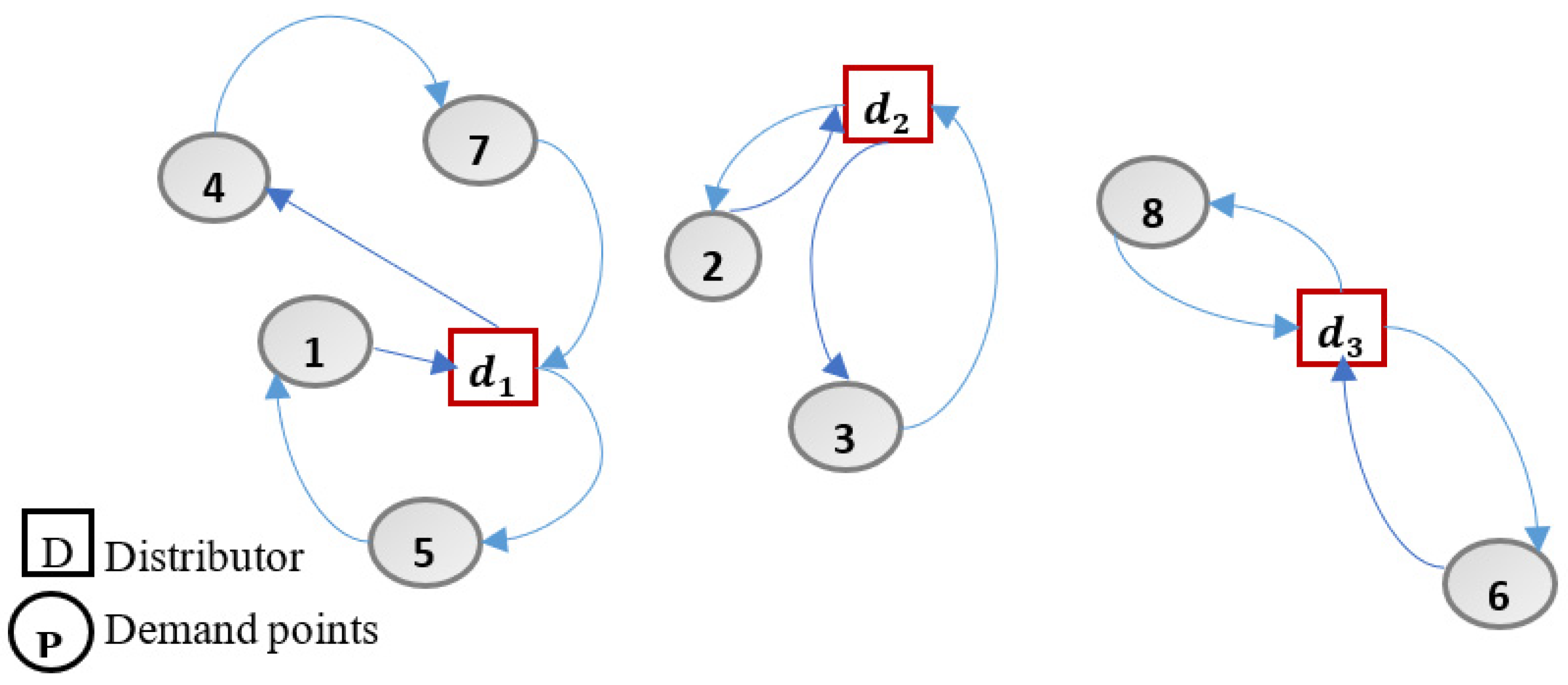
| 2 | 1 | 1 | 4-6-8 |
| 2 | 1 | 2 | 1-3 |
| 1 | 2 | 3 | 7-2-5 |
| NSGA-II | Value |
|---|---|
| npop | 50 |
| maxit | 400 |
| PC | 0.4 |
| Pm | 0.7 |
| Max UAS Characteristics | 1 m/Approx. 3 ft | 3 m/Approx. 10 ft | 8 m/Approx. 25 ft | >8 m/Approx. 25 ft |
|---|---|---|---|---|
| Typical kinetic energy Expected | <700 J (approx. 529 Ft Lb) | <34 KJ (approx. 25,000 Ft Lb) | <1084 KJ (approx. 800,000 Ft Lb) | 1084 KJ (approx. 800,000 Ft Lb) |
| Operational scenarios | ||||
| VLOS/BVLOS over controlled ground area | 1 | 2 | 3 | 4 |
| VLOS in sparsely populated environment | 2 | 3 | 4 | 5 |
| BVLOS in sparsely Populated | 3 | 4 | 5 | 6 |
| VLOS in populated Environment | 4 | 5 | 6 | 8 |
| BVLOS in populated Environment | 5 | 6 | 8 | 10 |
| VLOS over gathering of people | 7 | |||
| BVLOS over gathering of people | 8 |
| Importance Scale | Definition of Importance Scale |
|---|---|
| 1 | Equally important preferred |
| 2 | Equally to moderately important preferred |
| 3 | Moderately important preferred |
| 4 | Moderately to strongly important preferred |
| 5 | Strongly important preferred |
| 6 | Strongly to very strongly important preferred |
| 7 | Very strongly important preferred |
| 8 | Very strongly to extremely important preferred |
| 9 | Extremely important preferred |
| n | 1 | 2 | 3 | 4 | 5 | 6 | 7 | 8 | 9 | 10 |
|---|---|---|---|---|---|---|---|---|---|---|
| RC | 0 | 0 | 0.58 | 0.9 | 1.12 | 1.24 | 1.32 | 1.41 | 1.45 | 1.49 |
| RPA 1 | ||||||||
| 1 | 2 | 3 | 4 | 5 | 6 | 7 | 8 | |
| 1 | 167 | 60 | 28 | 87 | 176 | 56 | 234 | 34 |
| 2 | 117 | 39 | 40 | 83 | 123 | 34 | 256 | 47 |
| 3 | 123 | 121 | 22 | 22 | 147 | 78 | 278 | 67 |
| RPA 2 | ||||||||
| 1 | 147 | 78 | 36 | 90 | 144 | 43 | 246 | 46 |
| 2 | 123 | 43 | 57 | 61 | 187 | 45 | 215 | 67 |
| 3 | 136 | 134 | 17 | 15 | 245 | 81 | 209 | 89 |
| RPA 3 | ||||||||
| 1 | 193 | 56 | 28 | 84 | 148 | 57 | 296 | 59 |
| 2 | 119 | 68 | 57 | 62 | 197 | 43 | 257 | 54 |
| 3 | 142 | 123 | 19 | 14 | 223 | 79 | 211 | 68 |
| Number of Demand Points | NSGA-II | GAMS | ||||||
|---|---|---|---|---|---|---|---|---|
| Z1 | Z2 | Z3 | Elapsed Time(s) | Z1 | Z2 | Z3 | Elapsed Time(s) | |
| N = 4 | 449,297,460 | 10,004 | 9978 | 56.43 | 449,297,478 | 1049 | 9967 | 78.65 |
| N = 5 | 650,779,184 | 15,613 | 10,310 | 56.153 | 650,779,184 | 15,620 | 10,311 | 109.34 |
| N = 6 | 602,471,673 | 11,643 | 12,347 | 60.300 | 602,471,513 | 11,640 | 11,981 | 123.56 |
| N = 7 | 487,170,264 | 15,486 | 11,219 | 53.99 | 487,350,634 | 15,590 | 11,209 | 168.43 |
| N = 8 | 669,350,742 | 12,305 | 10,267 | 56.040 | 669,350,736 | 12,307 | 10,236 | 172.78 |
| N = 9 | 674,892,002 | 14,822 | 10,290 | 57.90 | 674,891,988 | 14,903 | 10,293 | 193.2 |
| N = 10 | 674,066,352 | 12,822 | 11,709 | 53.224 | 674,066,367 | 12,945 | 11,734 | 214.93 |
| Scenarios | PS | Optimal Solution | Activated Location | Z1 | Z2 | Z3 |
|---|---|---|---|---|---|---|
| 1 | 0.03 | 1 → (1,5)_(5,4)_(4,7) 2 → (2,3) 3 → (6,8) | 1,2,3 | 669,350,742 | 1.2305 | 10,267 |
| 2 | 0.04 | 1 → (1,5)_(5,4)_(4,7) 2 → (2,3) 3 → (6,8) |
| The Objective Function | Z1 | Z2 | Z3 |
|---|---|---|---|
| Z1 | 627,592,605 | 11,155 | 9311 |
| Z2 | 727,991,324 | 7321 | 9366 |
| Z3 | 820,942,970 | 14,059 | 8661 |
| Z1 (Cost) | Z2 (Time) | Z3 (Risk) | Cost () | Activate Location | Optimal Solution for Locations |
|---|---|---|---|---|---|
| 669,350,742 | 12,305 | 10,267 | 496 | 1,2,3 | 1 → (1,5)-(5,4)-(4,7) 2 → (2,3) 3 → (6,8) |
| 449,989,508 | 18,749 | 10,836 | 478 | 1,2,3 | 1 → (1,5)-(5,4)-(4,7) 2 → (2,3) 3 → (6,8) |
| 426,296,864 | 14,888 | 11,679 | 356 | 1,2,3,4 | 4 → (4,7) 2 → (2,3) 3 → (6,8) 1 → (1,5) |
| 412,789,234 | 19,329 | 11,345 | 280 | 1,2,3 | 1 → (1,5)-(5,4)-(4,7) 2 → (2,3) 3 → (6,8) |
| 367,879,215 | 21,354 | 11,236 | 130 | 1,2,3,4 | 4 → (4,7) 2 → (2,3) 3 → (6,8) 1 → (1,5) |
Publisher’s Note: MDPI stays neutral with regard to jurisdictional claims in published maps and institutional affiliations. |
© 2022 by the authors. Licensee MDPI, Basel, Switzerland. This article is an open access article distributed under the terms and conditions of the Creative Commons Attribution (CC BY) license (https://creativecommons.org/licenses/by/4.0/).
Share and Cite
Mahmoodi, A.; Hashemi, L.; Laliberté, J.; Millar, R.C. Secured Multi-Dimensional Robust Optimization Model for Remotely Piloted Aircraft System (RPAS) Delivery Network Based on the SORA Standard. Designs 2022, 6, 55. https://doi.org/10.3390/designs6030055
Mahmoodi A, Hashemi L, Laliberté J, Millar RC. Secured Multi-Dimensional Robust Optimization Model for Remotely Piloted Aircraft System (RPAS) Delivery Network Based on the SORA Standard. Designs. 2022; 6(3):55. https://doi.org/10.3390/designs6030055
Chicago/Turabian StyleMahmoodi, Armin, Leila Hashemi, Jeremy Laliberté, and Richard C. Millar. 2022. "Secured Multi-Dimensional Robust Optimization Model for Remotely Piloted Aircraft System (RPAS) Delivery Network Based on the SORA Standard" Designs 6, no. 3: 55. https://doi.org/10.3390/designs6030055