Article

Impacts of Location on Designs and Economics of DIY Low-Cost Fixed-Tilt Open Source Wood Solar Photovoltaic Racking

by
Nicholas Vandewetering
1,
Koami Soulemane Hayibo
2 and
Joshua M. Pearce
2,3,*
1
Department of Civil & Environmental Engineering, Western University, London, ON N6A 3K7, Canada
2
Department of Electrical & Computer Engineering, Western University, London, ON N6A 3K7, Canada
3
Ivey School of Business, Western University, London, ON N6A 3K7, Canada
*
Author to whom correspondence should be addressed.
Designs 2022, 6(3), 41; https://doi.org/10.3390/designs6030041
Submission received: 14 March 2022 / Revised: 13 April 2022 / Accepted: 18 April 2022 / Published: 21 April 2022
(This article belongs to the Topic Building Energy and Environment)

Abstract

:
Although small solar photovoltaic (PV) systems avoid most soft costs, they still have a relatively high $/W value due to racking costs. In order to fulfill the promise of small-scale plug-and-play solar, a do-it-yourself PV rack design is provided and analyzed here for six criteria: (1) made from locally-accessible renewable materials, (2) 25-year lifetime to match PV warranties, (3) able to be fabricated by average consumers, (4) able to meet Canadian structural building codes, (5) low cost and (6) that it is shared using an open-source license. The open-source wood-based fixed-tilt ground-mounted bifacial photovoltaic rack design evaluated here was found to be appropriate throughout North America. Economic analysis of the bill of materials showed the racking system ranges from 49% to 77% less expensive compared to commercial proprietary racking in Canada. The racking design, however, is highly dependent on the cost of lumber that varies widely throughout the world. Even for an absolute lower-cost design in Togo due to a lower fixed tilt angle and lower loads from lack of snow, it was not found to be economic because of the relatively high cost of wood. The recent volatile lumber market warrants local evaluation from those considering the use of the open-source design. This design, however, provides for a PV rack that can be manufactured with distributed means throughout most of the world enabling more equitable access to solar energy to support a circular bioeconomy.

Graphical Abstract

1. Introduction

Solar photovoltaic (PV) technology is a naturally distributed renewable energy technology that is well established as a leading sustainable energy source [1] because of an excellent ecological balance sheet [2,3,4]. The last remaining barrier to widespread PV deployment has been economic costs [5], but PV prices have dropped 60% in the last decade [6,7,8,9,10]. This has brought the levelized cost of solar electricity [11] is often the lowest cost option on a large scale [12,13]. Not surprisingly, PV is the most rapidly expanding electricity generation source [13,14]. Even when economies of scale are not in play, Levin & Thomas [15] showed that small solar home systems can play an important role in achieving U.N. ‘Sustainable Energy for All’ goals. In the developed world, most PV systems are grid-tied and there has been a surge of interest among consumers because they can effectively lower their electric utility bills with lower-cost solar electricity [16,17].
Even with clear lifetime economic benefits, however, the capital cost of a PV systems can be challenging for many consumers, particularly the poor, both in the developing [18] and the developed countries [19,20,21,22]. One approach to overcoming this challenge is to start with a small do-it-yourself (DIY) [23] or use plug-and-play solar, where PV modules are connected through microinverters directly to the household circuits by consumers. This latter approach is legal throughout some of Europe and is technically compliant with regulations in the U.S., although there is a widespread disparity in interpretations between the states and utilities [24,25]. Several studies have proposed methods to streamline the technology and regulations for such systems [25,26,27,28] because it would open up a large new market for PV to a wide range of consumers and potentially save Americans alone $13 billion/year [29].
Although these small DIY or plug-and-play systems avoid most of the soft costs associated with PV systems, they still have a relatively high $/W cost. This is because the majority of the cost declines in PV have come in the form of reduced PV module costs, while the relative cost of the balance of systems (BOS) has become more important [4,6,10]. The BOS consists of racking, electronics, and wiring. Racking, in particular, has been largely ignored in the peer-reviewed literature while the PV industry focused on various proprietary and costly aluminum extrusion profiles. Until recently, this was not important due to the fact that the relative costs of PV racking were marginal for the complete system and thus only modest progress was made in reducing PV racking materials and costs [30]. Because of this, current PV racking components can often dominate the costs of a PV system—particularly for smaller systems. For example, the low spot price for a PV module is currently US$0.19/W [31] while racking for a 3-module system costs US$535 (list price US$635) [32] which is US$1.78–0.45/W for 100 W and 400 W modules, respectively. Similarly, a 3-module pole mount is selling for US$1194, even with 400 W modules this is equivalent to about US$1/W for racking excluding the foundation [33].
Recently, several types of plastic-based PV racking have been proposed to reduce costs for low-tilt angle arrays, including: small-scale mobile PV arrays [34], flat roofs [35], ground-mounted systems at the equator in the developing world [36]. The vast majority of PV systems, however, have a much greater tilt angle, (e.g., approximately equivalent to the latitude). In addition, conventional racking materials for ground-mount systems (metal and concrete) have high embodied energies and play a major role in the environmental impact of a PV system [37]. Thus, in order to fulfill the promise of distributed DIY and plug-and-play solar, what is needed is a PV rack design that is; (1) made from locally-accessible sustainable renewable materials, (2) can be fabricated using simple hand tools by the average consumer, (3) has a 25-year life time to be equivalent to common PV warranties, (4) is structurally sound in order to weather high wind speeds and major snow loads (depending on the region), (5) has a low cost and (6) that it is shared using an open-source license so that many people can fabricate it themselves, or companies can make versions to offer in their local markets.
In order to overcome these challenges, this study reports on the technical and economic viability of an open-source DIY wood-based racking system. Specifically, a full structural analysis is completed for fixed-tilt wood-based PV racks developed following Canadian building codes for two locations: Ontario, Canada (to represent a northern latitude with heavy snow loads) and Togo (to represent a low-tilt angle system with no snow loads for locations close to the equator). The complete designs and bill of materials (BOM) of the racks are provided along with basic instructions and are released with an open-source license that will enable anyone to fabricate the rack system. The BOM costs are compared to the cost of proprietary commercial PV racks for both locations. The results of this study are discussed in the context of using an open-source DIY design for increasing PV deployments both in the global north and the global south.

2. Materials and Methods

All abbreviations are detailed in Abbreviations section.

2.1. Renewable Materials Selection for Racking: Wood

Wood was selected as a building material because it is locally available throughout most of the world. Choosing wood for the construction of PV racking can have both economic and environmental advantages. Unlike other construction materials, responsibly-sourced wood has the advantage of being sustainable [38], renewable, and comprised of approximately half carbon, which was recently taken from the atmosphere. When combined with lower energy needs for processing, wood actually has a negative combined embodied energy and carbon over alternative racking construction materials. For instance, aluminum (even with 31% recycled content), which is the most common PV racking material, has over 5 times the embodied CO2e/kg of wood [39], giving wood a distinctive advantage.
There are many choices, however, when it comes to wood species and how they might be treated for decay resistance. These are somewhat governed by local availability. Since the most common and easily available choice is treated softwood species it is reviewed here. Pressure-treating greatly extends the service life of wood and is commonly used on the fast-growing and more economical softwood species. Micronized copper azole is among the latest generation of wood preservatives and is considered safer than other preservative systems for humans, animals, and the environment [40]. Now, a common treatment used in residential settings, micronized copper azole, goes by many brand names, (e.g., MicroPro/LifeWood and Wolmanized Outdoor wood, Yellawood, and SmartSense). Micronized copper azole is also less corrosive on fasteners and can come into direct contact with aluminum, which is typically used in solar panel frames. Pressure-treated SPF (Spruce, Pine, Fir) lumber was selected because of its low cost, high availability, and overall durability in outdoor conditions. It is the most common wood used to construct decks, fences, gazebos, and other outdoor structures in Canada. Depending on the weather conditions, pressure-treated lumber can stay up for up to 40 years without signs of decaying [41].

2.2. Material Properties

There is a limited variety of dimensional lumber that can be used in building wooden structures. The dimensional properties of common structural lumber are summarized in Table 1. It should be noted that in all cases, the base should be less than the height so that the member is loaded in its strong axis, thus producing the optimal moment of inertia and the first moment of area values.
Where the cross-sectional area, A, in mm2 is calculated by,
A = b h
The moment of inertia, I, in mm4, for rectangular cross-sections is calculated by,
I = 1 12 b h 3
The first moment of area, Q, in mm3, for rectangular cross-sections is given by,
Q = h A 8

2.3. Case Studies

Two case studies were selected to demonstrate the wide range of potential PV system design situations. London, Ontario, Canada (42.9849° N, 81.2453° W) was selected as an example of a high-latitude location in the global north that would be expected to experience snow loading and need a substantial tilt angle. Lomé, Togo (6.1256° N, 1.2254° E) located near the equator was selected as a global south-based installation that would not have any snow-related losses nor necessitate designing for snow loads. The open-source System Advisory Model (SAM) [42,43,44] was used to determine the optimal fixed-tilt angle for both locations on an annual basis of energy production.
The optimal angle for London, Ontario for a fixed-tilt solar PV system according to SAM is 34° as shown in Figure 1a and for Lomé Togo is 10° as shown in Figure 1b.
These locations represent the extreme cases of a system in a location of high latitude and a system located by the equator. SAM can be used to determine the optimal angle for a location of any latitude. The optimal angle for locations with most of the human population is expected to be between these two extremes.

2.4. PV Racking Basic Design Parameters

The PV rack was designed to do a small system of ~1 kW so that it could be used for plug-and-play PV [25] and represent an initial cost that would be accessible to a greater population. A 400 W LG 400 W NeON2 BiFacial Solar Panel [45], was selected to take advantage of the bifacial PV rear surface solar absorption, which not only enhances electricity production [45,46,47] but also increases snow clearing on the front [48,49]. This racking system was specially designed for bifacial PV, but the design is still useful for any type of solar module. In regions where snow clearing or rear reflection are not of interest, bifacial modules can be substituted for any rigid framed module, which may further reduce the cost of the system. When selecting modules, it is important to ensure the module’s rear and front load capacities are greater than the design load calculated in Appendix A. The lumber structural capacities are shown in Appendix B. The approximate dimensions of the LG 400 W NeON2 modules are 1 m × 2 m. If modules with different dimensions are to be used, then the specifications in the assembly instructions in Section 3.1.2 can be scaled up or down to meet the given module’s requirements. Resizing the system will modify the design load calculated in Appendix A, which means smaller systems reduce costs by selecting smaller members such that no limits are exceeded in the structural analysis outlined in Appendix C.
In order for the racking to be widely applicable, they are designed to be ground-mounted and have a 500 mm ground clearance to avoid obstructing snow slide-off even in extreme northern environments [50]. The tilt angle is 34° for London, Ontario, and 10° for Lomé, Togo. Both systems are designed to withstand 80 mph winds and the London racking system must be able to handle typical snow load as well. These were chosen as extreme conditions so that if the system could withstand the mechanical loads in these conditions, it would be able to handle any loads in less severe environments. Following open hardware design guidelines [51,52,53] the design is released under CERN Open Hardware License V2 strong reciprocal variant (CERN-OHL-S) [54].

2.5. Design Analysis Assumptions

The snow, wind, and dead loads are calculated and combined for both case study designs following Appendix A. The structural analysis calculations are shown in Appendix B. Many common assumptions must be made to simplify and idealize the structural analysis. It should be noted that these assumptions are conservative, meaning that they further ensure that the structure will not fail unexpectedly.
  • All loads shall act perpendicular to the face of the modules, so joists are experiencing the worst-case flexural load.
  • All members are idealized as pins connected with no fixed end moments since joist hangers and brackets still allow for rotation [55].
  • The wind load and snow load will only be applied to the surface of the modules because the accumulation of snow on wooden members is practically negligible.
  • The wind load and snow load are assumed to be distributed evenly throughout the surface of the modules because snow and wind accumulation is only considered for large structures as per NBCC 4.1.6 [56].
  • The modules can be idealized as a one-way slab since the length to span ratio is 2 [57].
  • The modules used for these systems are the LG NeON 2 from Volts Energies in Quebec. According to the supplier, the modules can endure a front load of up to 5400 Pa, and a rear load of up to 4000 Pa [45]. Since the design loads will be much less than these values, the modules will have sufficient structural capacity.

2.6. Economic Analysis

The economic cost of the solar PV wood racking equipment for Togo is obtained locally. The dimensions of the wood pieces are converted into metric units and used for pricing. In Togo, and the Western Africa region in general, one type of wood that is widely available and suitable for use in racking is teak wood [58,59]. Togolese teak is not pressure-treated, but it is naturally resistant to water. Furthermore, the lumber is usually treated using a water-resistant varnish that allows it to be used in outdoor applications. Because of the lack of strict enforcement of the regulations on local wood costs, the price varies from one vendor to another, and an average price has been used in this study. Additionally, the cost of the connection equipment is obtained from local vendors in Togo.
The comparison between the cost of the different racking systems is done on a 3-module basis, a per W basis, and extended to the levelized cost of electricity (LCOE). The percent differences for each are given. The costs of these DIY wooden racking systems are compared to the cost of both commercial and residential DIY metal racking in Canada and Togo. This comparison is important because in Togo, for non-utility grade solar PV systems, the racking is usually manufactured locally using steel that is treated with water-resistant paint. It should be noted that commercial systems are typically not sold in three module systems and will usually include the modules in their pricing. Thus, the cost of commercial metal racking systems, minus the commercial cost of modules, is converted to a cost per W basis, and then multiplied by the 1200 W in 3 bifacial modules [volts.ca] to calculate a cost per 3-module basis. The LCOE of the racking is obtained by dividing the cost of the racking by the lifetime energy production of the system. The lifetime energy production of the system is obtained by performing a SAM simulation using the optimal tilt angles for Canada and Togo, respectively, as shown in Figure 1. The SAM simulation is performed by considering bifacial solar modules, a system lifetime of 25 years, and a module degradation rate of 0.5%/year [60].
After the calculation of the cost of wood racking for London, Ontario, the result is compared to that of a design with no snow load. The no snow load case is provided as the projections for snow losses are substantially decreased with climate change future projections even over the relatively medium-term (e.g., 2040) [61].

3. Results

Following the design procedure outlined in the previous section, two wood-based fixed-tilt wood-based racks were designed for both case study locations.

3.1. London, Ontario: 34 Degree Fixed Racking System

3.1.1. Bill of Materials

The bill of materials (BOM) of the London, Ontario system is shown in Table 2 in Canadian dollars sourced from Copp’s Build-All, London, or Home Depot, London.

3.1.2. London Assembly Instructions

The system requires at least two builders to install. Refer to Table 3 for the typical time spent completing each component per two builders.
To begin, four holes at least 250 mm in diameter are dug at least 1.2 m into the ground to prevent frost heaving of any soil type according to Table 9.12.2.2 in the National Building Code of Canada (NBCC) [56]. The holes are spaced according to Figure 2 from center to center. The front posts are made by cutting one 4 × 4 × 10 into two pieces at 1.6 m. The back posts are made by cutting each 6 × 6 × 8 to a length of 2.7 m. If concrete is being used for the footings, mix two bags of 30 kg Quikrete ready-mix concrete with water in a wheelbarrow. The mix should be evenly distributed under and around the posts. Once the hole is filled, dug-up topsoil should be used to cap the dug hole to ensure water slopes away from the footing as shown in Figure 3. Refer to instructions provided on the bag to ensure the mix cures to a serviceable hardness before continuing construction.
Two 2 × 8 × 10 beams cut into 3 m pieces are to be installed as shown in Figure 4a. Use 2-1/2” brown deck screws to tighten the connection between the beams and the posts. Two 1/2” holes are drilled through the posts and beams as seen in Figure 4b, and 6” and 8” carriage bolts are inserted for the 4 × 4 and 6 × 6 posts, respectively. All carriage bolts are to be tightly secured with a washer and nut as shown in Figure 4c.
A 2 × 4 bracing must be installed to enhance the system’s stability. Two 2 × 4 × 8 s are cut to 1.6 m to install from front post to back post, 300 mm above the ground as seen in Figure 5a. Another 2 × 4 × 8 is cut to 2 m to be installed between the first 2 × 4 s in the middle of the system, about 750 mm from the front posts. All 2 × 4 s are installed as shown in Figure 5b with 2 × 4 galvanized fence brackets and 1-1/2” joist hanger nails for stronger and more ductile connections. 2-1/2” brown deck screws should be used to further sink the 2 × 4 into the post, and to improve the connection’s resistance to pullout.
The outside joists are made from 2 × 6 × 8 s, and the inside joists are made from 2 × 8 × 8 s as shown in Figure 6a. A miter saw is adjusted to cut the joists to an angle of 34 degrees, and pieces are cut to 1.95 m. The joists are spaced 1 m from each other as shown in Figure 6b. Additional fence brackets are used for the bracing to install the joist to beam connections. The bottom lip of the bracket can be bent to align with the 34-degree angle. Four brown deck screws per beam should be installed as shown in Figure 6c to further sink the joist into the beam, and to improve load transfer between the members.
Once the joists are installed, scrap pieces of lumber can be cut into blocks and installed onto the joists with two screws as shown in Figure 7a. These blocks serve as the connection between the module and the lumber and can be adjusted to match the holes of the module frame. The overhang of these blocks shall not exceed 100 mm. Once these blocks are installed, the modules can be placed onto the blocks. Drill a ¼” hole through the bottom of the block, and insert a ¼” × 2 − 1/2” galvanized bolt from under the system. Then, place the module onto the bolt, and secure the connection with a nut and washer as shown in Figure 7b. To enhance the load transfer to the joist, place another block under the overhanging block, and screw the second block into the joist as shown in Figure 7c.
Once all connections are secured, the build is complete (Figure 8). The system can then be disassembled in the reverse order it was initially constructed.
Following the calculations shown in Appendix B for the structural analysis, the forces and deflections of the fixed angle system specifically for the London, Ontario system have been summarized in Table 4. When constructing a system, it is important to follow the structural design process in Appendix B to ensure the system can withstand the design load outlined in Appendix A. Depending on the design load, smaller members can be selected, and thus the net cost of the system can be reduced such that the maximum shear, moment, deflection, and axial forces are less than the capacities shown in Table A7 of Appendix B.

3.2. Lomé Togo 10 Degree Fixed Rack

3.2.1. BOM 10 Degree Fixed Rack

The bill of materials (BOM) of the Lomé Togo system is shown in Table 5 in Canadian dollars (CAD) to compare to Table 2.
The values in Togo found in Table 6 are converted to $CAD where 1 $CAD = 457.800 XOF [62] so the total with no concrete is $507.63 and with concrete, it is $540.10, which is 39% percent more than building in Canada.

3.2.2. Lomé, Togo Fixed Rack Installation Instructions

The post installation process for the Togo system is the same as the fixed-angle process in Canada. The spacing of posts changes with a fixed tilt angle so that it shall correspond to the center to center spacing shown in Figure 9.
The beam, bracing, joist, and block installation are the same process as the 34-degree fixed rack. The miter saw should be set at 10-degree cuts when cutting the joists.
The 10-degree (Figure 10) structural analysis process is identical to the 34-degree structural analysis. Lomé, Togo’s design load is half of London, Ontario’s design load, thus, analysis results were half of London Ontario’s analysis results.

3.3. Economic Analysis

The cost per 3-module basis, cost per W, and LCOE for each system have been summarized in Table 7.
The material costs for the open-source wood rack for London, ON Latitude purchased in Canada, is CAD$388.78. The cost per installed W for this system is CAD$0.32/W, which corresponds to an LCOE of CAD$0.010/kWh. Subtracting the cost of the footings (which do not come with any commercial systems) the cost is CAD$348.94, which is CAD$0.29/W. Using a US$ to $CAD of 1.28 [64] for comparison, 3-module system costs CAD$682.83 [32] using the same PV is CAD$0.57/W and a 3-module pole mount rack is CAD$1523.93 [33] is CAD$1.27/W. Other Canadian racking systems available on the market fall between this range. Even when scaled up to a 12-module system (4 of these OS wood designs) the cost is CAD$0.32/W, while commercial systems cost CAD$3430.75 [65] or CAD$0.71/W. Thus, the percent savings for small systems range from 49% to 77% and this also leaves the open-source wood rack less expensive (17% savings) than residential roof racking costs of CAD$0.35/W [66].
The 10-degree design that does not need to handle snow loads is CAD$309.69; however, if the wood is purchased in Togo, it increases to CAD$540.10. The impact that wood prices have on this design is substantial. In Togo, the availability of an extremely inexpensive DIY metal rack (CAD$165) coupled with the much higher cost of wood, makes it uneconomic. It should be noted there is no structural stability study behind the design of the locally manufactured steel racking in Togo.
For a no snow load design, when following the design load procedure outlined in Appendix A, a London, Ontario system with a fixed tilt angle of 34 degrees will have a design load of approximately 0.83 kPa, which is practically the same design load as Lomé, Togo’s design load of 0.81 kPa. Thus, the no snow system can be built with the same BOM as the wooden Togo system at a cost of CAD$309.69. A no snow load design results in a price reduction of about 20%.
The Canada and Togo systems represent the two extreme cases of a system being used in a location of high latitude and a location near the equator. Therefore, a system anywhere in the world will have a cost roughly between these two extreme cases. The cost of any given system is dependent on the region’s wind and snow load, which can be calculated using Appendix A, and the cost of lumber in the region, which is further discussed in Section 4.2.

4. Discussion

4.1. Limitations

For the wood members, regardless of the preservative system chosen or available, the buried wood posts must be rated for a below-ground application, while the upper structure can be rated for ground contact or lower. The higher the rating, the more preservative chemicals are in the wood, and normally the higher the cost. More information and resources for homeowners can be found American Wood Protection Association (awpa.org). A treated wood solar rack can last a lifetime common to the PV warranties of 25 years if installed in accordance with manufacturers’ instructions. This typically includes hand treating exposed board cuts and drilled holes with a 2% copper naphthenate solution (commonly available at home improvement stores, lumber yards, or online). In addition, particular care must be taken if the installation is in a higher wood deterioration zone. The Forestry Chronicle provides a decay hazard map showing high hazards of decay off the coast of British Colombia [67]. The American Wood Protection Association (AWPA) provides a decay hazard zone map showing high hazard decay in California, and the south [68]. As all materials come to an end of their service lives, treated wood must be disposed of properly, which usually means taking it to a landfill or transfer station. The material should not be burned or reused as mulch so there is a need for future work to find an environmentally benign method of recycling treated wood such as low-temperature pyrolysis [69].
To avoid the use of treated wood, there are species that offer natural decay resistance. White oak (Quercus alba) offers impressive strength and decay resistance [70] and would be suitable for long life in most solar racking applications. White oak also has slightly better mechanical properties [71] than red oak. Additionally, white cedar and western red cedar are commonly available at hardware stores for approximately 2.5 times the cost of pressure-treated wood. This again pushes the wood rack to become uneconomical with the current cost of metal.
The footings of the system can be made with concrete, or any other type of ground-rated mixture to hold the posts in place. However, the mixture should have a compressive strength of at least 30 MPa to ensure it can withstand ground stresses due to freeze–thaw cycles if put in cold environments [72]. For warm regions in which freeze–thaw cycles will not be problematic, a minimum compressive strength of 20 MPa is required [72]. To make a 20 MPa mix, use a water to cement ratio of 0.70 instead of the typical ratio of 0.55. Additionally, the air content of the mixture should not exceed 8% to ensure water does not induce too much internal stress in the mix. These compressive strength requirements lend the opportunity to work with alternative building materials, which are left for future work. All hardware used in the system, such as nails, screws, brackets, bolts, etc., shall be either hot-dipped galvanized, electrogalvanized, or stainless steel to ensure a lifetime of 25 years. Although common zinc plated hardware is inexpensive and easily accessible, it cannot be used for outdoor applications.

4.2. Wood Price Sensitivity

Although the open-source wood-based PV rack provided substantial savings in Canada and was able to be constructed with no special tools, the same was not found in Togo. The system is highly sensitive to the price of lumber, which recently has been volatile and increasing as shown in Figure 11. Once a sustainable equilibrium is reached, the costs of this design could decrease by a factor of 2–3 as shown by the earlier years in Figure 11. This would make the substantial savings observed in the Canadian market even more striking and allow for the system to compete with the low-cost metal racks in Togo.
The costs of this design in all parts of the world will also be dependent on the local sources of wood being available and if imported the taxes and import duties. Considering all of these issues and the results of this study, the open-source wood rack has the potential to be less expensive than proprietary offerings everywhere but is highly situation-dependent. Refer to Table 7 for the typical price of a construction grade pressure treated 2 × 4 × 8 in various countries around the world, which shows the impact of international import duties and material availability. As can be seen in Table 8—the two case studies selected represented both the high (Togo) and relatively low (Canada) costs of wood globally.
The cost of pressure-treated lumber is noticeably higher in other continents compared to the cost in North America. This makes it more difficult to observe the economic benefits of using wood for PV racking globally, but once sustainable equilibrium is reached, the cost of a wood system can prove to be competitive with metal systems on a global level.
As per Section 1.3.1.1 Div. A of the Ontario Building Code [56], a building inspection and permit for a ground-mounted system is not required. A grid-connected PV system may require an inspection from the Electrical Safety Authority [74]. These rules depend on locality and may change as PV obtains high grid penetration rates [75].
Future work can further refine the design to make a rack specific for: (1) monofacial PV (which would use less wood as the cross members could go behind the module back surface and decrease lumber lengths), (2) multi-tilt angle capability, (3) vertical racks and (4) investigate at the impact of the designs on a greater number of woods and recycled plastic lumber. In addition, the use of strategic bracing or wire tension can also be explored for reducing the materials needed. Wood racking should also be evaluated for viability for use in spray cooling PV systems [76].
In addition, a full life cycle analysis is needed to determine if this design, although able to be made with sustainably harvested wood, is indeed ecologically superior to more traditional metal-based racking designs. This analysis can include all the externality costs and evaluate the system for on-grid, off-grid, and microgrid [77]. All of this work supports the potential for further reducing the costs and applications of open-source PV racks.

5. Conclusions

Wood can be a sustainable source of photovoltaic system racking materials to support a circular bioeconomy. The open-source wood-based fixed-tilt ground-mounted bifacial photovoltaic rack design evaluated here is appropriate throughout North America. The results found the open-source wood rack contributes only 1.1 US cents to the LCOE and can be fabricated for roughly 49% to 77% less than proprietary small-scale metal racks. Although the design of the system needs fewer materials in regions that do not experience snowfall, this may or may not equate to lower capital costs. This is because the system is highly dependent on the costs of lumber. For designers attempting to optimize both the LCOE as well as the environmental impact of PV systems, wood may be a viable lower-cost option than conventional racking materials. As wood costs come back towards historic norms, wood PV racking provides a promising method to further improve the economical footprint for PV systems anywhere in the world. Lastly, this design provides for a rack that can be manufactured with a distributed means throughout most of the world enabling more equitable access to solar energy.

Author Contributions

Conceptualization, J.M.P.; methodology, N.V., K.S.H.; software, K.S.H.; validation, N.V., K.S.H.; formal analysis, J.M.P., N.V., K.S.H.; investigation, N.V., K.S.H.; resources, J.M.P.; data curation, N.V., K.S.H.; writing—original draft preparation J.M.P., N.V., K.S.H.; writing—review and editing, J.M.P., N.V., K.S.H.; visualization, N.V., K.S.H.; supervision, J.M.P.; funding acquisition, J.M.P. All authors have read and agreed to the published version of the manuscript.

Funding

This research was funded by Thompson Endowment.

Institutional Review Board Statement

Not applicable.

Informed Consent Statement

Not applicable.

Data Availability Statement

Data will be made available upon request.

Acknowledgments

The authors would like to thank Paul Vandewetering of Paul’s Build-All for assistance in the construction of the 34-degree rack. In addition, the authors would like to thank Tao Bentho and Komi Jacques Gakli-Gaka for providing equipment costs for Togo.

Conflicts of Interest

The authors declare no conflict of interest. The funders had no role in the design of the study; in the collection, analyses, or interpretation of data; in the writing of the manuscript, or in the decision to publish the results.

Abbreviations

Structural Analysis
wUniform distributed load
LMember length
VmaxMaximum Shear Force
MmaxMaximum Bending Moment
ΔmaxMaximum Deflection
Design Loads
SDesign Snow Load
ISSnow Importance Factor
SSGround Snow Load Factor
CbBasic Roof Snow Load Factor
CWWind Exposure Factor
CSSlope Factor
CaAccumulation Factor
SrRain Factor
WDesign Wind Load
IwWind Importance Factor
q1/50 Year Wind Pressure
CeExposure Factor
CpCgPressure and Gust factor
CeiInternal Exposure Factor
CgiInternal Gust Factor
CpiInternal Pressure Factor
DDesign Dead Load
Material Properties
bCross-Sectional Base
hCross-Sectional Height
ACross-Sectional Area
IMoment of Inertia
QFirst Moment of Area
fbFlexural Resistance
fvShear Stress Resistance
ftTensile Stress Resistance
fcCompression Stress Resistance Parallel to the grain
EElastic Modulus
EminMinimum Elastic Modulus
CdDuration Factor
CtTemperature Factor
CLBeam Stability Factor
CMWet Service Factor
CfuFlat Use Factor
CiIncising Factor
CfMember Size Factor
fb*, fv*, ft*, fc*, E*Factored Resistances
MrFactored Bending Moment Resistance
VrFactored Shear Force Resistance
TrFactored Tensile Force Resistance
CrFactored Compression Force Resistance
DfootingDiameter of ground footing

Appendix A. Specified Loads

Appendix A.1. Snow Load NBCC 4.1.6

The governing snow load [56] is composed of multiple factors shown in Equation (A1),
S = I s [ S s ( C b C w C s C a ) + S r ]
The Importance Factor, IS, is taken as 0.8 because the failure of a PV system has little to no risk of the loss of life.
The Ground Snow Load Factor, SS, is dependent on the location of the structure. It is the 1-in-50-year snow load found in Table C-2 in NBCC 4.1.6 For London, Ontario, a value of 1.90 must be taken [56].
The Basic Roof Snow Load Factor, Cb, is 0.80 for small structures.
The Wind Exposure Factor, Cw, is taken as 0.75 if the structure is exposed to wind in all directions.
The Slope Factor, Cs, is dependent on the tilt angle of the system. It can be calculated using the following equation from NBCC 4.1.6.
C S = 60 a n g l e 45
The Accumulation Factor, Ca, is taken as 1.00 for small monoslope structures.
The Rain Factor, Sr, depends on the location of the structure. For London, Ontario, a value of 0.40 must be taken according to Table C-2 in NBCC 4.1.6 [56].
The factors and calculated net snow load are summarized in Table A1.
Table A1. Design Snow Load. Note that the minimum specified snow load is to be taken as 1.00 kPa.
CoefficientValue
Is0.80
Ss1.90 1
Cb0.80
CW0.75
CS0.58 2
Ca1.00
Sr0.40 1
S0.85 3
1 This value is specific to London, Ontario. Refer to Table C-2 in NBCC 4.1.6 for other locations. 2 This value is specific to 34-degree systems. Refer to Equation X for other angles. 3 As per NBCC, the minimum specified design snow load shall not be less than 1.00 kPa.

Appendix A.2. Wind Load

The specified wind load is adapted from the National Building Code of Canada 2015, Division B, 4.1.7, and is composed of both an external wind pressure, and internal wind pressure,
W = p + p i
where the external wind pressure is composed of the following factors,
p = I w q C e C t C p C g
The internal wind pressure is composed of the following factors,
p i = I w q C e i C t C g i C p i
The Wind Importance Factor, IW, is taken as 0.80 because the failure of a PV system has little to no risk of the loss of life.
The Hourly Wind Pressure Factor, q, is dependent on the location of the structure. It is the 1-in-50-year wind load found in Table C-2 in NBCC 4.1.6 For London, Ontario, a value of 0.47 must be taken.
The Exposure Factor, Ce, shall be taken as 0.90 for structures less than 10 m in height.
The topographic factor, Ct, is to be taken as 1.00.
The Pressure and Gust Factors, Cp and Cg, are combined and found using the table from Figure 4.1.7.6-A from NBCC [56]. From the figure, the governing building for 34-degree systems is 2, which corresponds to a CpCg value of −1.30.
The Internal Exposure Factor, Cei, is the same as the External Exposure Factor, Ce since the structure has a “dominant opening”, meaning that wind can attack the inside of the system just as easily as it can attack the outside.
The Internal Gust Factor, Cgi, is taken as 2.00 since is not a large unpartitioned volume, such as an arena.
The Internal Pressure Factor, Cpi, will be taken as −0.70 because the wind has easy access to push against the back of the system.
The factors and calculated net snow load are summarized in Table A2.
Table A2. Design Wind Load as per NBCC 4.1.7.3.
CoefficientValue
IW0.80
q0.47
Ce0.90
Ct1.00
CpCg−1.30
Cei0.90
Cgi2.00
CPi−0.70
p−0.44
pi−0.47
W−0.91 kPa

Appendix A.3. Specified Dead Load

The dead load, or the self-weight of the structure, will consist of the weight of the PV modules, and the weights of the wooden members. The weight of brackets and fasteners is much smaller than the design load and can be considered negligible. According to Natural Resources Canada’s CanmetENERGY research centre [78], a dead load of PV systems, also known as the superimposed dead load, shall be taken as 0.24 kPa. The self-weight of the lumber depends on what dimensions of lumber has sufficient capacity to carry the load. The self-weight of lumber is variable due to changing moisture content and amount of knots. For analysis purposes, it is best practice to use the lumber weights provided by the supplier, and translate the given weight into a uniform distributed load in kN/m.

Appendix A.4. Load Combinations

Since many simple assumptions are made in the analysis process, safety factors must be applied to the specified loads to reduce the probability of failure. These factored loads are then combined as principle loads and companion loads via the load combinations found in NBCC 4.1.3.2 [56]. The combination of principal loads and companion loads that creates the largest net load shall be used in the analysis. Principle loads are the mandatory loads that must be checked, and companion loads are only added if they act in the same direction as the principal loads. Since the design wind load acts in the negative direction and the governing snow load is in the positive direction, they shall not be combined as doing so will reduce the net load. The combinations that produced the largest positive and negative are found in Table A3.
Table A3. Load Combinations as per NBCC 4.1.3.2. Based on Design Dead, Snow, and Wind Loads.
CombinationNet Load [kPa]
0.9D 1 + 1.4W−1.06
1.25D + 1.5S1.80
1 A factor of either 0.9 or 1.25 can be used for the dead load D. Since the wind load W acts in the opposite direction as D, 0.9 is selected to create the maximum negative net load.
It should be noted that the load path for the positive case is the same as the negative case, the only difference being the direction of the load. Since all connections can resist loads in both directions, and all members have the same material properties in both directions, the analysis for the negative case is the same as the positive case. Thus, the negative case can be ignored, and the positive case will be used for the analysis.
The same process will be applied to a system located in Lomé, Togo. For this system, it is justified to assume that the snow load is 0 kPa. All wind coefficients can be the same as the London, Ontario system with the exception of q and CpCg because they depend on the wind speed and tilt angle, respectively. The hourly wind pressure q for Lomé, Togo, is not readily tabulated, but can be calculated using the wind pressure Equation (A6) shown below,
q = 1 2 ρ V 2
where ρ is the density of air, and V is the 1-in-50 year wind speed. NBCC suggests taking a ρ value of 1.29 kg/m3 [56]. According to the European Conference on Severe Storms 2019, V for Lomé, Togo will be taken as 20 m/s [79]. Plugging these values into the equation, q becomes 0.26 kPa.
CpCg for 10 degrees turns out to be −1.30 as well, thus producing a net wind load of −0.42 KPa. The governing load combination for this system is 0.9D + 1.4W, which produces a specified design load for this system to be −0.81 KPa.

Appendix B. Lumber Structural Capacity

The material properties of lumber are extremely variable due to the multiple different species of wood, the existence of knots that alter the load path in the member, and the fluctuating moisture content carried inside the wood. The National Design Speciation for Wood Construction 2018 [80] provides engineers with trustworthy design values for the vast majority of wood species. Almost all pressure-treated lumber in Canada is made of Spruce Pine Fir grades number 1 and 2 [81], which possess the structural capacities summarized in Table A4.
Table A4. Unfactored capacities for No. 1/2 Spruce Pine Fir Lumber.
CapacityValue [MPa]
fb6.03
fv0.93
ft3.10
fc7.93
E9652.60
Emin3516.30
Although these capacities have proven to be reliable, resistance factors must be applied to the capacities to account for unexpected weaknesses and to ensure a safe and serviceable design.
The load duration factor, Cd, is selected as 1.15 since the snow load is the governing load on the structure.
The temperature factor, Ct, is 1.00 since the structure will not be exposed to temperatures over 100 degrees Fahrenheit.
The beam stability factor, CL, is calculated as 0.98 as per the guidelines outlined in Appendix C of the NDS.
The wet service factor, CM, is calculated as 1.00 because the product of fb and Cf is less than 7.9.
The flat use factor, Cfu, is 1.00 because all members are to be loaded upon their strong axis in which h > b.
The incising factor, Ci, is selected as 0.8 as per Table 4.3.8 in the NDS [80].
The repetitive member factor, Cr, is 1.00 since the structure cannot be considered a floor or roof system with multiple of the same member.
Finally, the size factor, Cf, is selected as 1.00 because lumber greater than 2 × 12 will not be used for this design.
These factors have been summarized in Table A5,
Table A5. Resistance factors as per the National Design Specification for Wood Construction.
CoefficientValue
Cd1.15
Ct1.00
CL0.98
CM1.00
Cfu1.00
Ci0.80
Cr1.00
Cf1.00
As per the National Design Specification for Wood Construction, the factored bending capacity is calculated as,
f b * = f b [ C D C t C L C M C f u C i C r C F ]
The factored shear stress is calculated as,
f v * = f v [ C D C M C i ]
The factored tensile stress is calculated as,
f t * = f t [ C D C M C f C i ]
The factored compressive stress is calculated as,
f c * = f c [ C D C M C t C f C i ]
Finally, the factored elastic modulus is calculated as,
E * = E [ C M C t C i ]
These factored capacities have been summarized in Table A6.
Table A6. Factored capacities for No. 1/2 Spruce Pine Fir Lumber.
Factored CapacityValue [MPa]
fb*5.44
fv*0.86
ft*2.85
fc*7.29
E*9169.97
Using the factored capacities and dimensional properties, resistance values can be computed using the following equations,
The resisting bending moment, Mr, can be calculated as,
M r = 2 f b * I h
The resisting shear force, Vr, can be calculated as,
V r = f v * I b Q
The resisting tensile force, Tr, can be calculated as,
T r = f t * A  
The resisting compressive force, Cr, can be as,
C r = f c * A
Resisting values for each dimensional lumber have been summarized in Table A7.
Table A7. Resisting values for No. 1/2 Spruce Pine Fir Lumber.
LumberMr [kN·m]Vr [kN]Tr [kN]Cr [kN] 1
2 × 40.271.939.6524.66
2 × 60.673.0315.1838.79
2 × 81.173.9919.9550.98
2 × 101.905.0925.4865.12
2 × 122.826.2031.0179.25
4 × 40.644.5222.6057.76
6 × 62.4911.1855.92142.92
1 Compression resistances are for loads parallel to the wood grain.
To ensure that the structure does not fail, the following conditions must be met for each member:
The resisting bending moment must be greater than or equal to the maximum applied bending moment,
M r M m a x
The resisting shear force must be greater than or equal to the maximum applied shear force,
V r V m a x
The resisting tensile force must be greater than or equal to the maximum applied tensile force,
T r T m a x
The resisting compressive force must be greater than or equal to the maximum applied compressive force,
C r C m a x
Finally, the maximum deflection cannot exceed the member length divided by 360 as per NBCC 9.4.3 [NRC],
L / 360 Δ m a x
Now that a design load and material properties are given, structural analysis can be conducted to determine the optimal dimensions of lumber needed to build a serviceable system.

Appendix C. 34 Degree Fixed System Structural Analysis

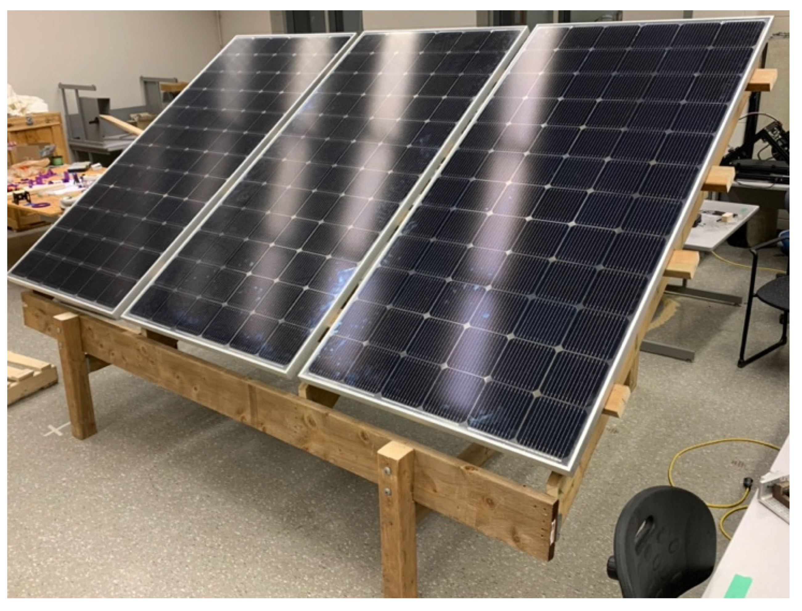
The net load is distributed evenly throughout the surface of the modules. As per the supplier of the modules [volts.ca], it is assumed that the panels have sufficient capacity to carry these loads. The load is then transferred from the panels to the joists. Each joist carries its own weight as a uniform distributed load, w, and 4-point loads that represent the block connections. w is calculated using Equation (A21),
w = 1.25 ( O W )
OW represents the own weight of the member, which needs to be multiplied by a factor of 1.25 because it is a dead load [82]. Since the required dimensions of lumber to carry the load is unknown, an assumption needs to be made (for example, assume 2 × 8) to carry out the analysis. If the assumption results in the maximum applied value being greater than the resistance values, then a larger member needs to be used.
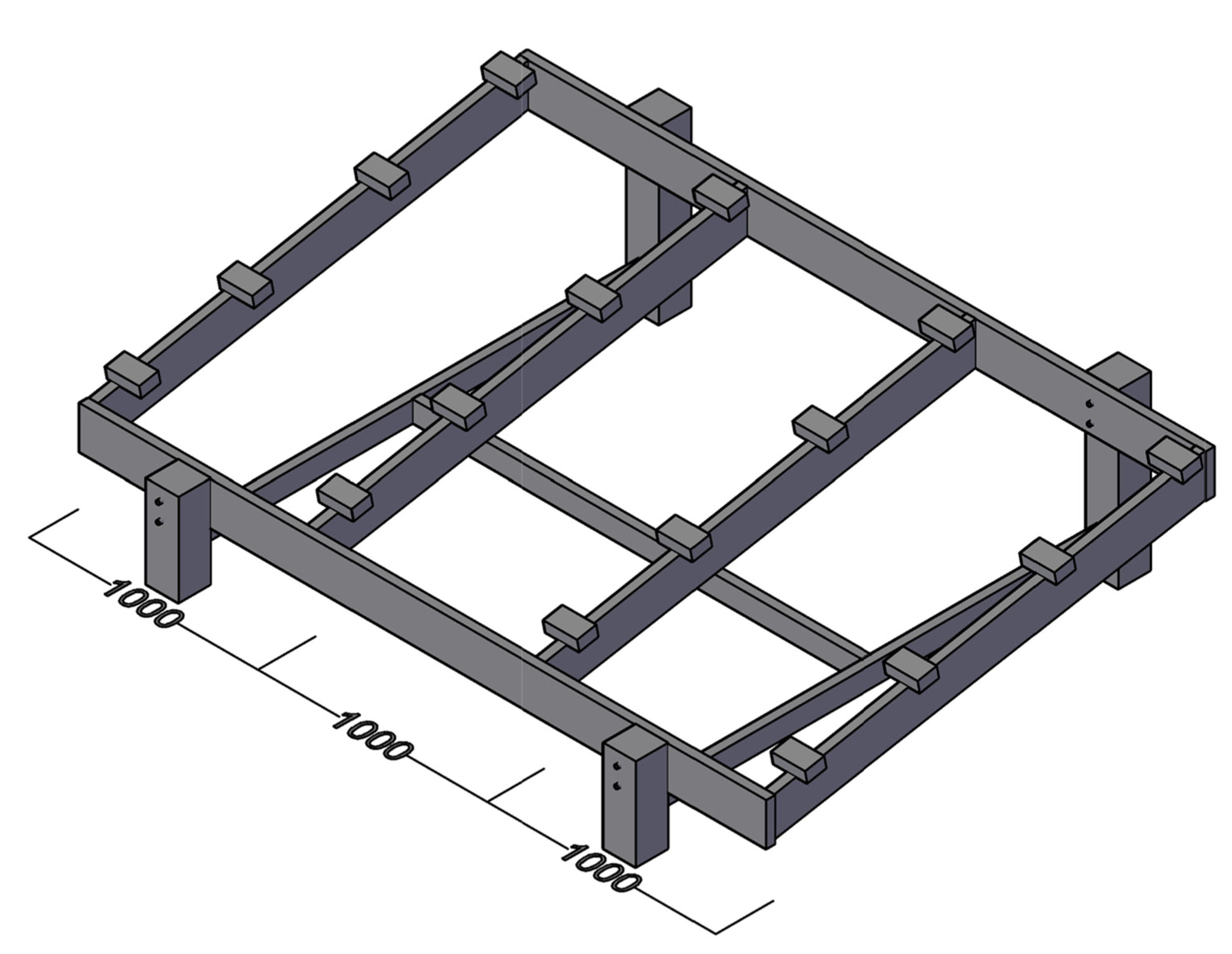
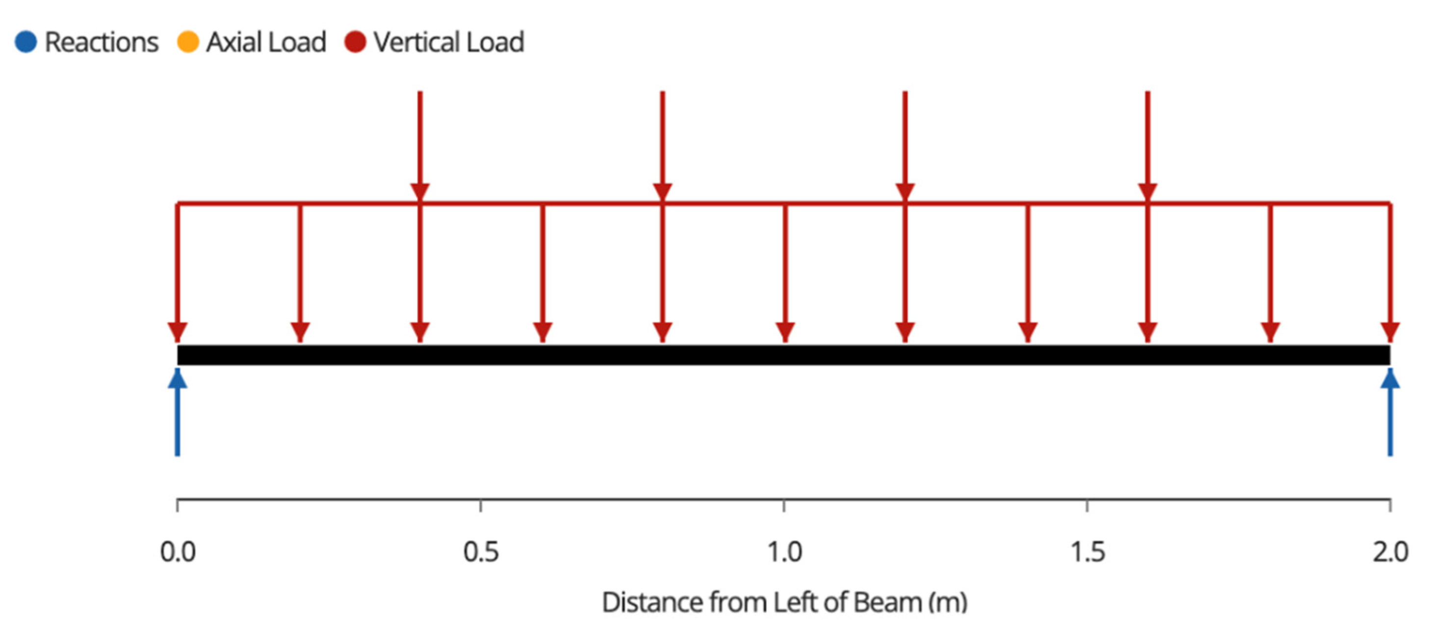
The point loads can be calculated by dividing each joist’s tributary loading into four points because it is assumed that the load is distributed evenly throughout the modules. The tributary area represents how much width of the panels each joist is responsible for carrying. For example, in this three-module system, which is 3 m wide, the middle joists have a tributary width of 1 m (0.5 m on each side), and the end joists have a tributary width of 0.5 m (only one side). The value for each point load on the joists is calculated as,
P o i n t   L o a d = D e s i g n   L o a d × T r i b u t a r y   A r e a 4
Once w and the point loads are calculated, the free body diagram for each joist can be made (Figure A1),
Figure A1. Free body diagram of joists. Note that the two outside joists will have half the tributary area of the inside joists, and thus will carry approximately half of the load.
Designs 06 00041 g0a1
Each joist is supported by a beam on each end. The reaction, and thus the load that each joist transfers to each beam is the following,
R e a c t i o n = 4 P o i n t   L o a d + w L 2
The shear force diagram throughout each joist is the seen as Figure A2,
Figure A2. Joist Shear Force Diagram.
Designs 06 00041 g0a2
The maximum shear force occurs at the supports, and thus the maximum shear is calculated as the reaction shown above.
The bending moment diagram in each joist is seen as Figure A3,
Figure A3. Joist Bending Moment Diagram.
Designs 06 00041 g0a3
The maximum bending moment of the joists occurs at the midspan. The maximum bending moment can easily be calculated by
M m a x = w L 2 8 + 3 ( P o i n t   L o a d ) L 5
The deflection diagram throughout each joist is seen as Figure A4,
Figure A4. Joist Deflection Diagram.
Designs 06 00041 g0a4
The maximum deflection of the joists occurs at the midspan. For simplicity of analysis, assume the 4-point loads serve as a uniform distributed load and calculate the maximum deflection using the following equation,
Δ m a x = 5 ( w + 2 ( P o i n t   L o a d ) L 4 384 E I
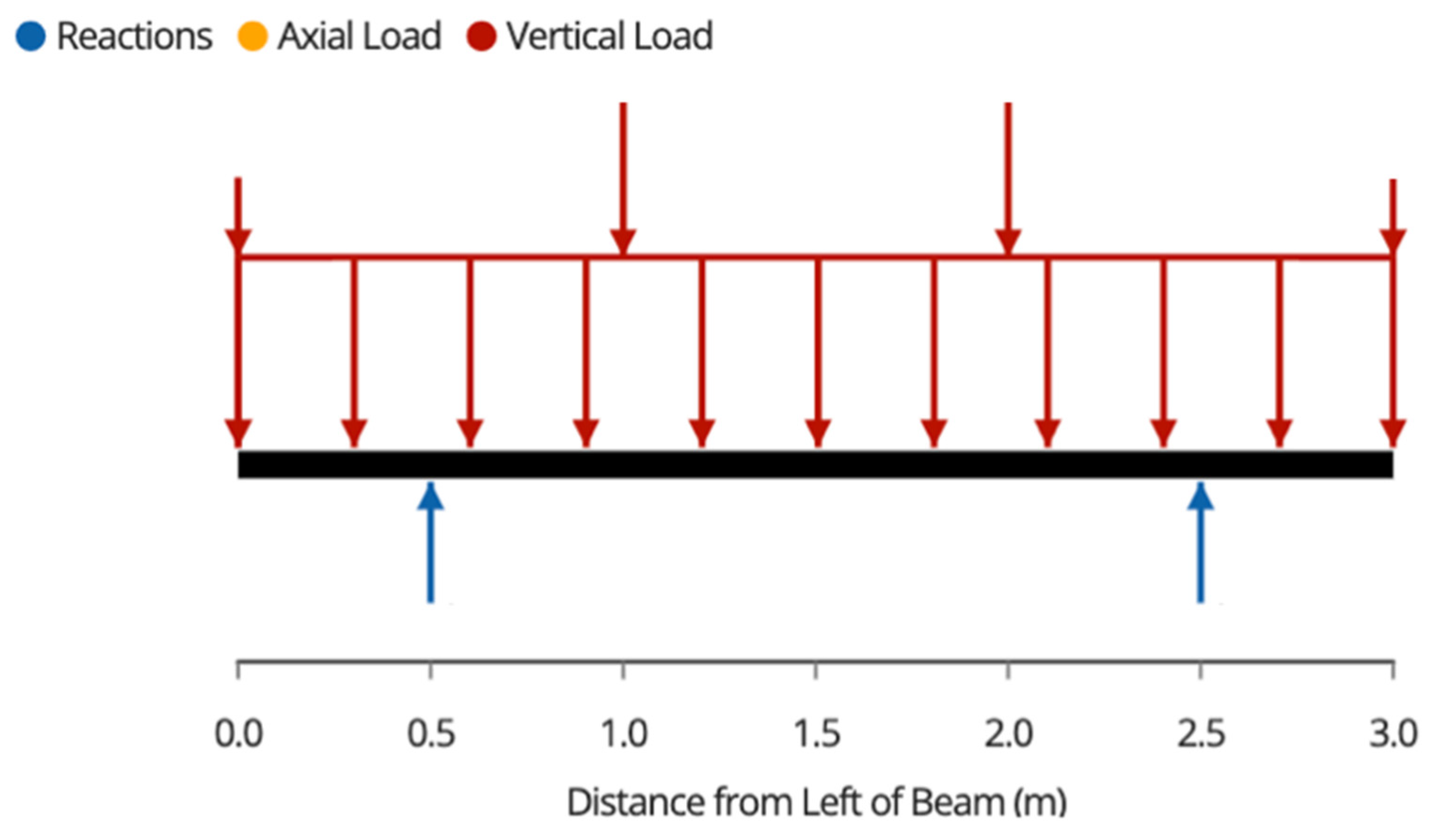
The beams then carry the point loads of each joist and the factored own weight of the member. The free-body diagram is described in Figure A5,
Figure A5. Beam Free-Body Diagram.
Designs 06 00041 g0a5
Due to the symmetric loading of the beams, the post loads, or the support reactions are described as,
R e a c t i o n = ( k = 1 4 J o i s t   R e a c t i o n s ) + w L 2
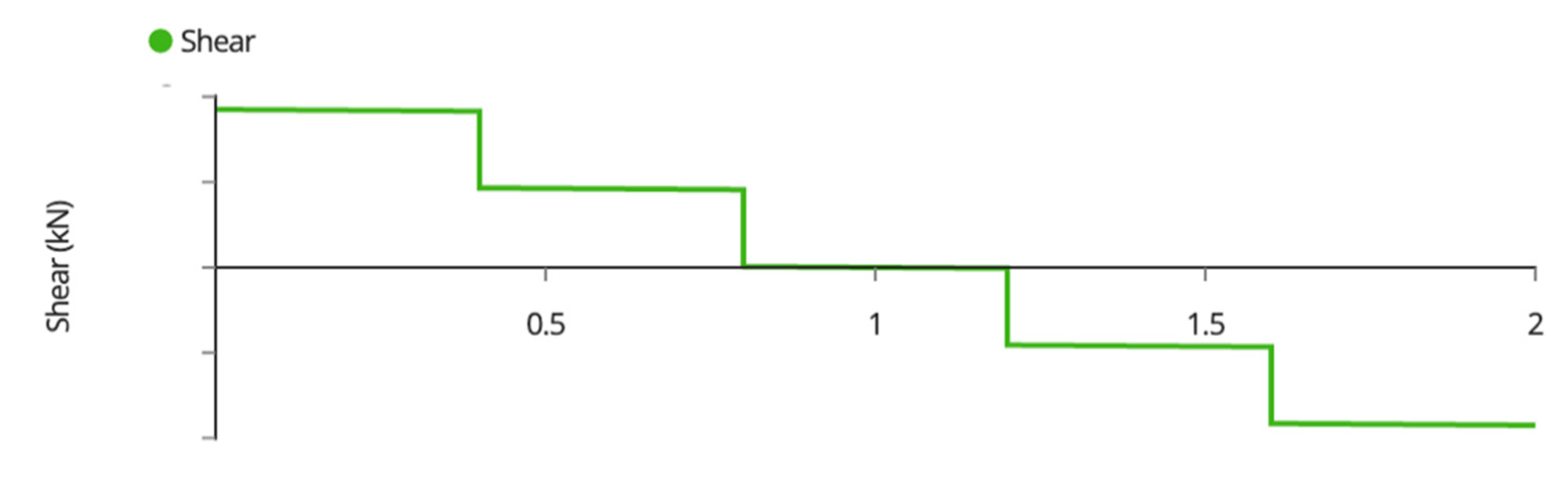
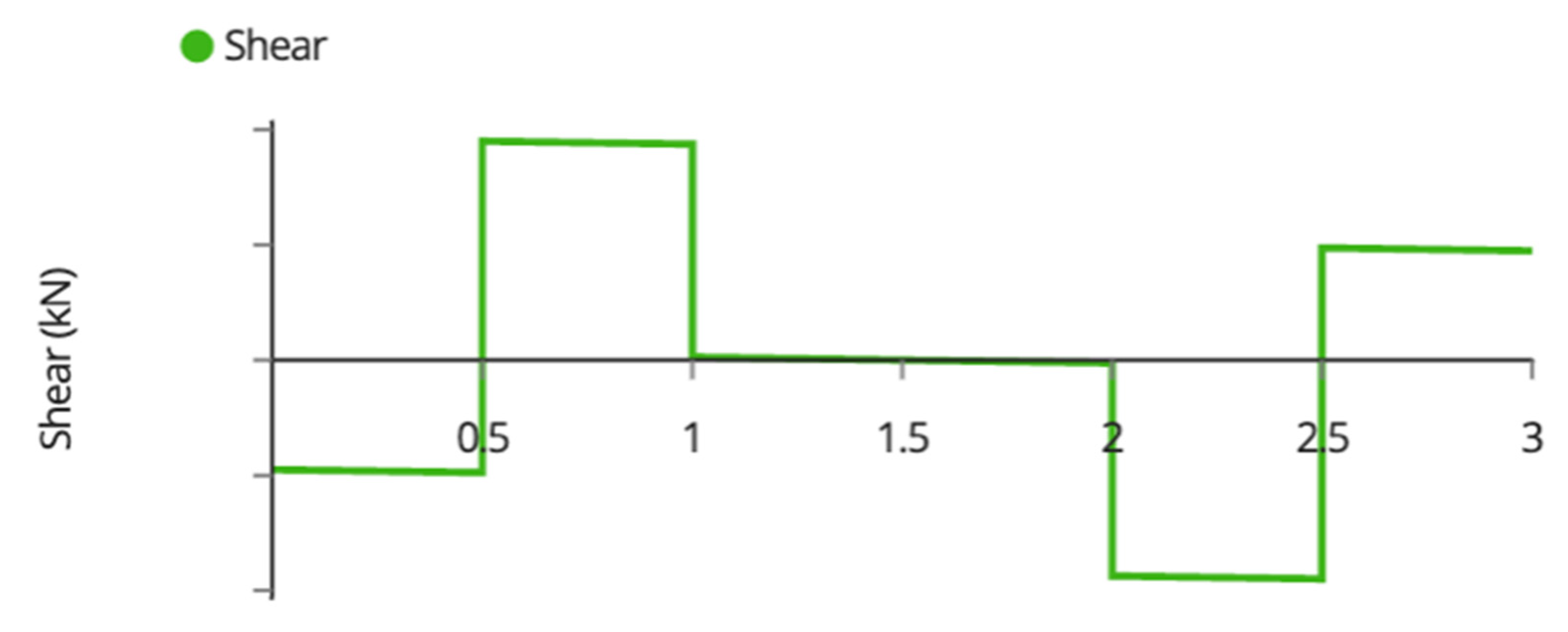
The shear force diagram for the beams is described in Figure A6,
Figure A6. Beam Shear Force Diagram.
Designs 06 00041 g0a6
The maximum shear forces occur on the inside of the reactions with a value of,
V m a x = R e a c t i o n J o i s t   L o a d 1 w L 6
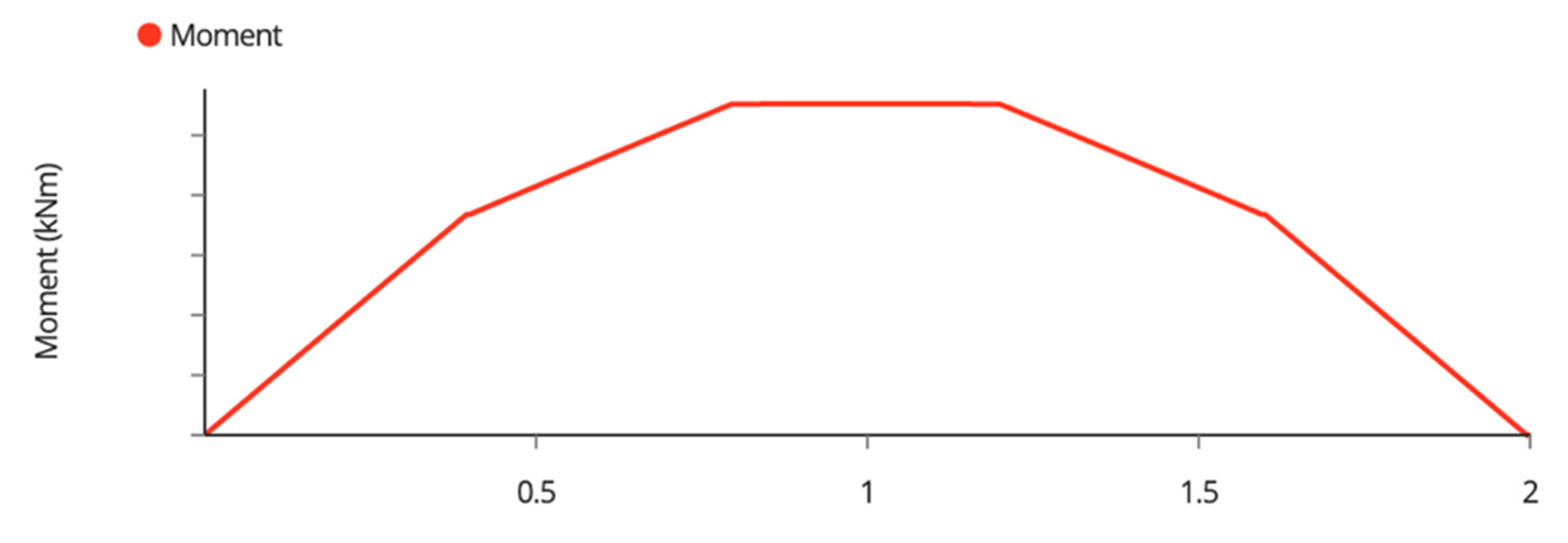
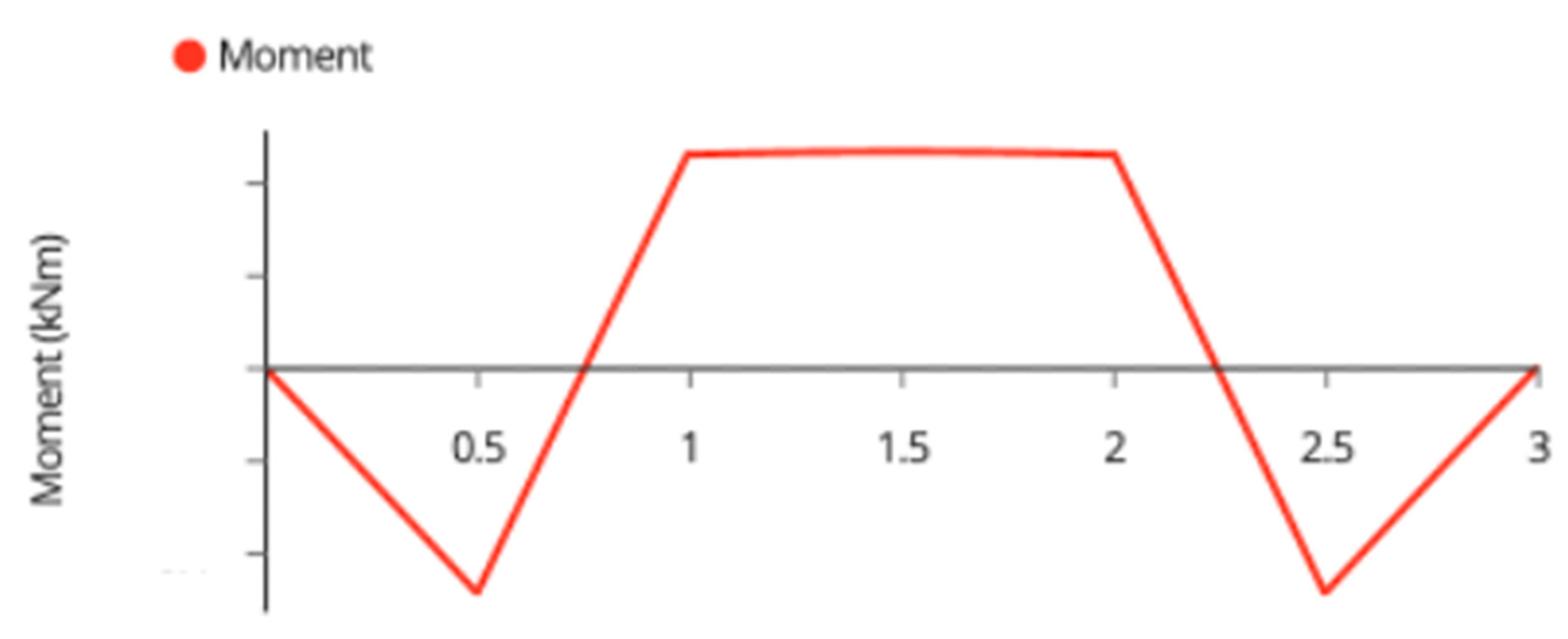
The bending moment diagram for the beam is shown in Figure A7,
Figure A7. Beam Bending Moment Diagram.
Designs 06 00041 g0a7
The maximum moment occurs at the supports and can be found by integrating the shear force throughout the first sixth of the beam as described in Equation (A28), or by simply finding the area under the shear force diagram.
M m a x = 0 L / 6 V ( x ) d x = ( J o i s t   L o a d 1 ) L 6 + w L 2 72
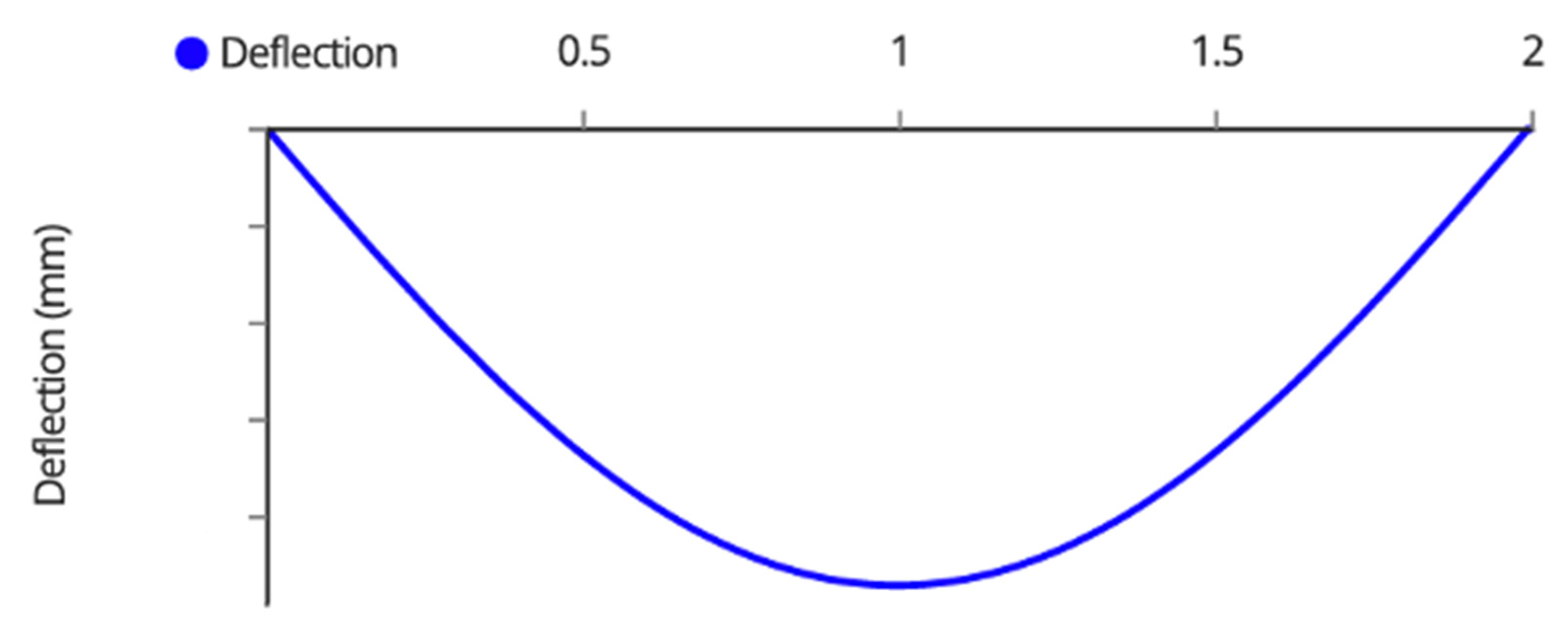
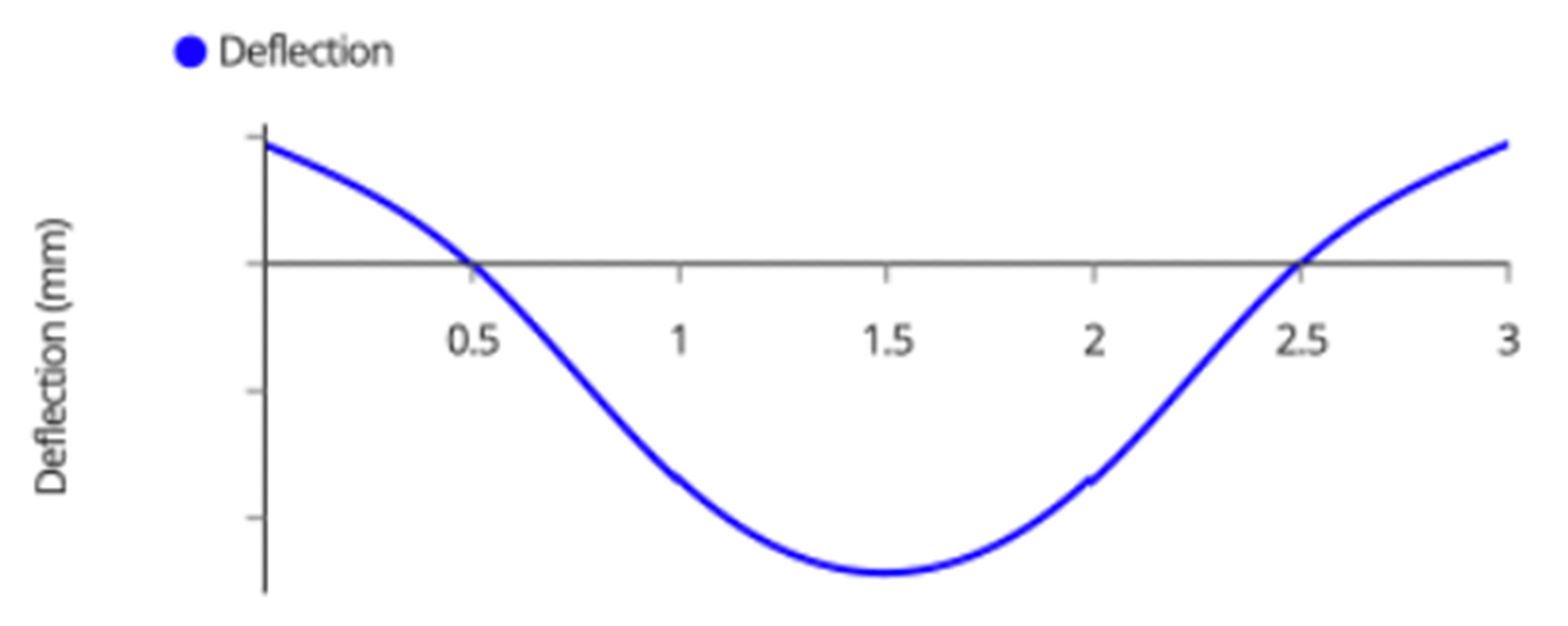
The deflection diagram is shown in Figure A8,
Figure A8. Beam Deflection Diagram.
Designs 06 00041 g0a8
The maximum deflection occurs at midspan and can be solved using the differential equation and initial conditions below, or by using the moment area theorem or virtual work method described in many structural engineering textbooks.
d 2 Δ d x 2 = M ( x ) E I Δ ( L 3 ) = 0 Δ ( L 2 ) = 0
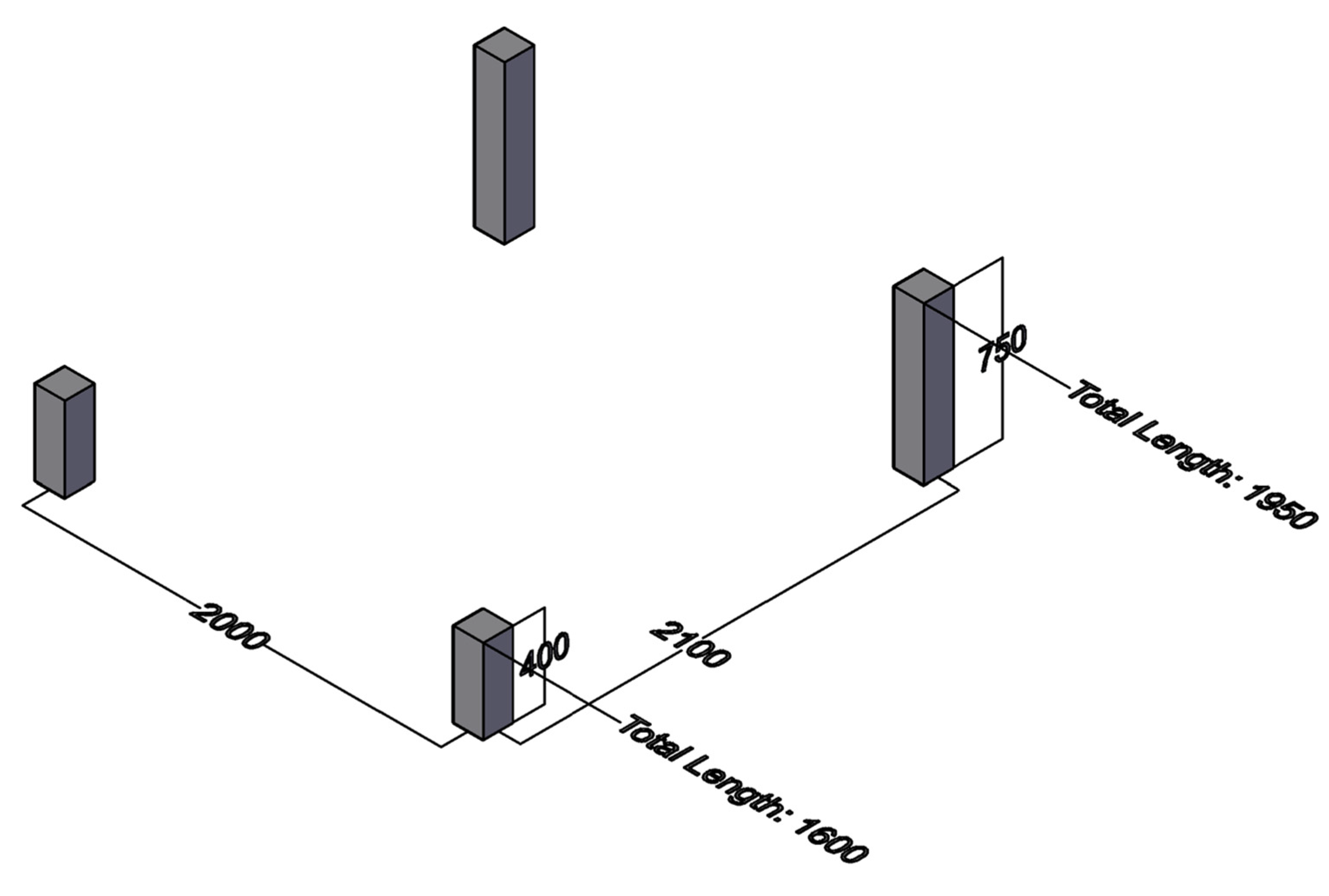
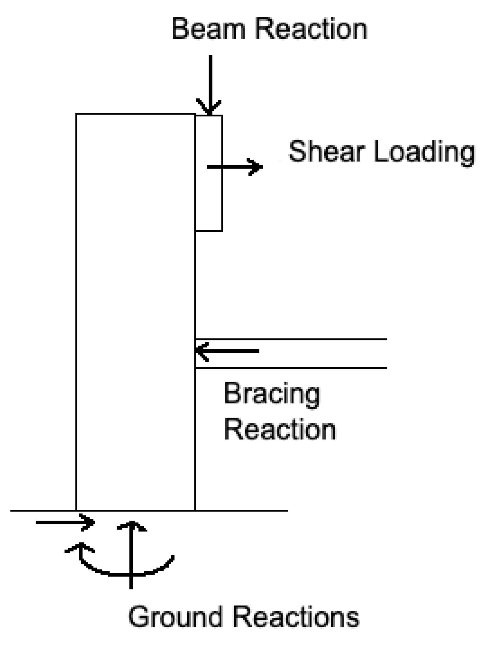
The load is then transferred to the posts. It should be noted that the posts are not loaded purely in compression; an eccentricity described in the free body diagram in Figure A9 induces a bending moment. The post can be idealized as a cantilever with a support reaction from a 2 × 4 brace.
Figure A9. Post Free Body Diagram.
Designs 06 00041 g0a9
The compressive load of the column is equal to the beam reaction solved above. Along with this compressive load comes a shear loading that is induced by wind and snow loads. This loading can act in either the left or right direction, but the load should be analyzed in the direction that induces bending in the same direction as the beam reaction for assessment of the critical case. The magnitude of this shear load in each post is described in Equation (A30),
S h e a r   L o a d = ( D e s i g n   L o a d ) cos ( θ ) 4
where θ is the tilt angle of the system. It should be noted that this cantilever with bracing support is an indeterminate structure, meaning that it has too many supports to be solved with static analysis, and thus can not be expressed with generalized equations. The structure can be solved by using finite element analysis, or by an analytical method such as the moment distribution or slope-deflection method.
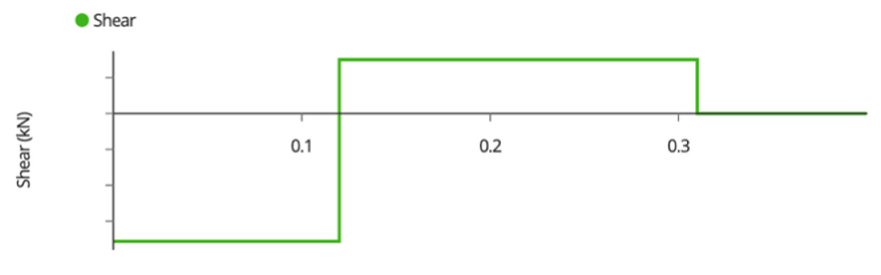
The shear force diagram of the post is seen in Figure A10,
Figure A10. Post Shear Force Diagram.
Designs 06 00041 g0a10
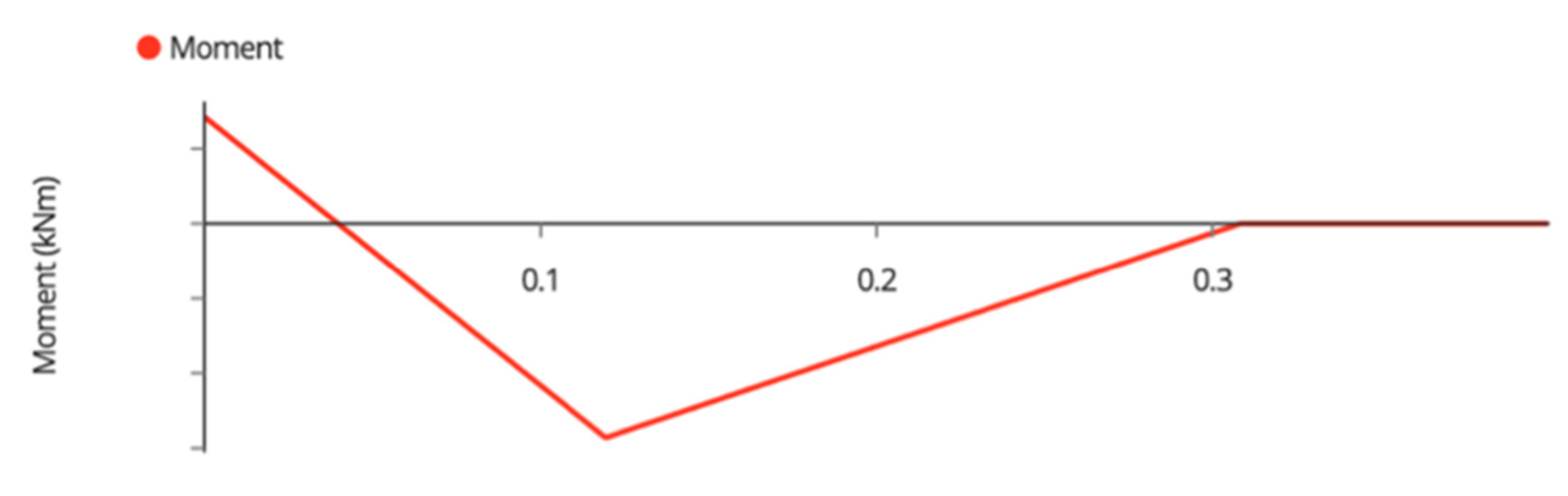
The bending moment diagram of the post is seen in Figure A11,
Figure A11. Post-Bending Moment Diagram.
Designs 06 00041 g0a11
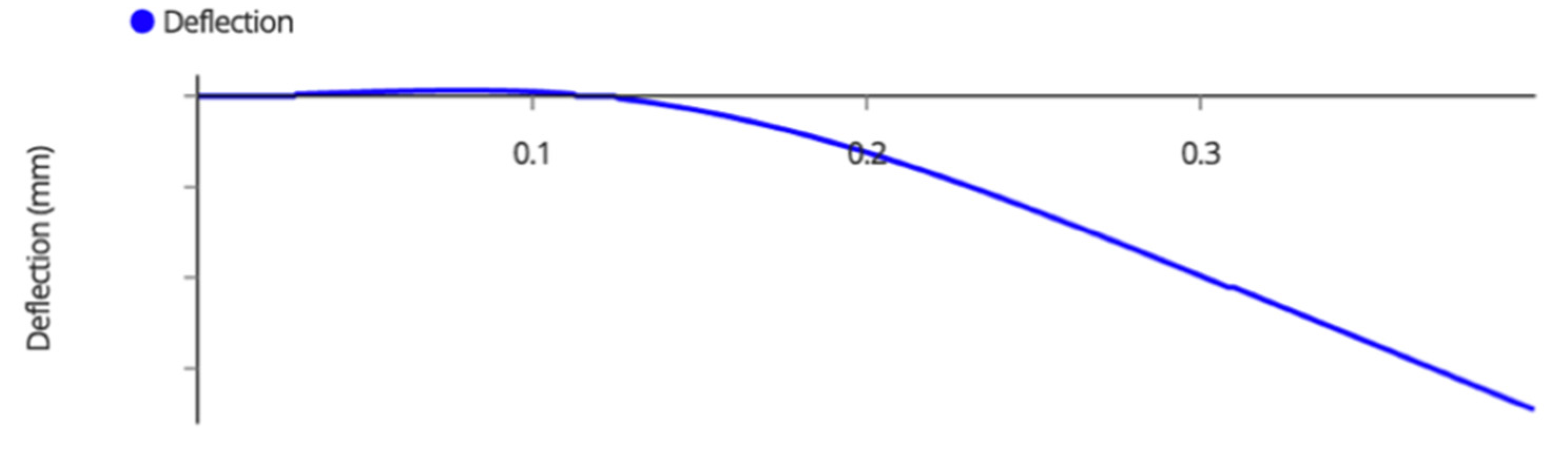
The deflection diagram of the post is seen in Figure A12,
Figure A12. Post Deflection Diagram.
Designs 06 00041 g0a12
The 2 × 4 brace support is a slender compression member. Not only should the applied force be less than the compressive resistance, but should be less than the buckling resistance governed by the following Euler Buckling equation,
C b u c k l i n g = π 2 E I w e a k L 2
w h e r e   I w e a k = 1 12 h b 3
Once all components of the post have been analyzed, the load will finally transfer itself to the ground. Table 9.4.4.1 of the NBCC provides maximum allowable bearing pressures for different types of soil and rock [56]. In the worst case, soft clays support a maximum bearing pressure of 75 kPa. To ensure, that the ground is not overloaded and settles, the bearing pressure can be calculated with the following equation,
B e a r i n g   P r e s s u r e = P o s t   C o m p r e s s i o n π 4 ( D F o o t i n g ) 2
If the applied pressure is more than the allowable, 150 mm of compacted clear stone gravel can be added to the bottom of the footing, or the footing diameter can be increased.
Throughout the system, each connection transfers the load from one member to another via a shear force within the fasteners that compose that connection. For bolts complying with ASTM A307A, the shear resistance of a ½” carriage bolt holding the beams is about 23.8 kN, and the shear resistance of a ¼” carriage bolt holding the modules is 5.21 kN [83], both of which are beyond the demand of these systems, and thus will not be critical to the design.

References

  1. Pearce, J.M. Photovoltaics—A path to sustainable futures. Futures 2002, 34, 663–674. [Google Scholar] [CrossRef]
  2. Fthenakis, V.M.; Moskowitz, P.D. Photovoltaics: Environmental, health and safety issues and perspectives. Prog. Photovolt. Res. Appl. 2000, 8, 27–38. [Google Scholar] [CrossRef]
  3. Pearce, J.; Lau, A. Net energy analysis for sustainable energy production from silicon based solar cells. In ASME Solar 2002: International Solar Energy Conference; American Society of Mechanical Engineers Digital Collection: Little Falls, NJ, USA, 2002; pp. 181–186. [Google Scholar]
  4. Fthenakis, V.; Alsema, E. Photovoltaics energy payback times, greenhouse gas emissions and external costs: 2004—Early 2005 status. Prog. Photovolt. Res. Appl. 2006, 14, 275–280. [Google Scholar] [CrossRef] [Green Version]
  5. Barbose, G.L.; Darghouth, N.R.; LaCommare, K.H.; Millstein, D.; Rand, J. Tracking the Sun: Installed Price Trends for Distributed Photovoltaic Systems in the United States-2018 Edition; Electricity Markets & Policy: Berkeley, CA, USA, 2018. [Google Scholar]
  6. Feldman, D.; Barbose, G.; Margolis, R.; Bolinger, M.; Chung, D.; Fu, R.; Seel, J.; Davidson, C.; Darghouth, N.; Wiser, R. Photovoltaic System Pricing Trends: Historical, Recent, and Near-Term Projections 2015 Edition; National Renewable Energy Lab.: Golden, CO, USA, 2015. [Google Scholar]
  7. Fu, R.; Feldman, D.J.; Margolis, R.M. US Solar Photovoltaic System Cost Benchmark: Q1 2018; No. NREL/TP-6A20-72399; National Renewable Energy Lab. (NREL): Golden, CO, USA, 2018. [Google Scholar]
  8. Barron, A.R. Cost reduction in the solar industry. Mater. Today 2015, 18, 2–3. [Google Scholar] [CrossRef] [Green Version]
  9. Reuters. Solar Costs to Fall Further, Powering Global Demand—Irena. Reuters 2017. Available online: https://www.reuters.com/article/singapore-energy-solar-idUSL4N1MY2F8 (accessed on 13 April 2020).
  10. Matasci, S. Solar Panel Cost: Avg. Solar Panel Prices by State in 2019: EnergySage. Solar News, EnergySage, 5 June 2019. Available online: news.energysage.com/how-much-does-the-average-solar-panel-installation-cost-in-the-u-s/ (accessed on 28 January 2022).
  11. Branker, K.; Pathak, M.J.M.; Pearce, J.M. A review of solar photovoltaic levelized cost of electricity. Renew. Sustain. Energy Rev. 2011, 15, 4470–4482. [Google Scholar] [CrossRef] [Green Version]
  12. Dudley, D. Renewable Energy Will Be Consistently Cheaper Than Fossil Fuels By 2020, Report Claims [WWW Document]; Forbes: Jersey City, NJ, USA, 2019; Available online: https://www.forbes.com/sites/dominicdudley/2018/01/13/renewable-energy-cost-effective-fossil-fuels-2020/ (accessed on 13 April 2020).
  13. Solar Industry Research Data. Available online: https://www.seia.org/solar-industry-research-data (accessed on 13 April 2020).
  14. Vaughan, A. Time to Shine: Solar Power Is Fastest-Growing Source of New Energy. Available online: https://www.theguardian.com/environment/2017/oct/04/solar-power-renewables-international-energy-agency/ (accessed on 28 January 2022).
  15. Levin, T.; Thomas, V.M. Can developing countries leapfrog the centralized electrification paradigm? Energy Sustain. Dev. 2016, 31, 97–107. [Google Scholar] [CrossRef] [Green Version]
  16. Lang, T.; Ammann, D.; Girod, B. Profitability in absence of subsidies: A techno-economic analysis of rooftop photovoltaic self-consumption in residential and commercial buildings. Renew. Energy 2016, 87, 77–87. [Google Scholar] [CrossRef]
  17. Prehoda, E.; Pearce, J.; Schelly, C. Policies to Overcome Barriers for Renewable Energy Distributed Generation: A Case Study of Utility Structure and Regulatory Regimes in Michigan. Energies 2019, 12, 674. [Google Scholar] [CrossRef] [Green Version]
  18. Agenbroad, J.; Carlin, K.; Ernst, K.; Doig, S. Minigrids in the Money: Six Ways to Reduce Minigrid Costs by 60% for Rural Electrification. Rocky Mountain Institute. 2018. Available online: https://rmi.org/insight/minigrids-money/ (accessed on 28 February 2022).
  19. Alafita, T.; Pearce, J.M. Securitization of residential solar photovoltaic assets: Costs, risks and uncertainty. Energy Policy 2014, 67, 488–498. [Google Scholar] [CrossRef] [Green Version]
  20. Rai, V.; Reeves, D.C.; Margolis, R. Overcoming Barriers and Uncertainties in the Adoption of Residential Solar PV. Renew. Energy 2016, 89, 498–505. [Google Scholar] [CrossRef]
  21. Horváth, D.; Szabó, R.Z. Evolution of Photovoltaic Business Models: Overcoming the Main Barriers of Distributed Energy Deployment. Renew. Sustain. Energy Rev. 2018, 90, 623–635. [Google Scholar] [CrossRef]
  22. Yousaf, H.; Shakeel, S.R.; Rajala, A.; Raza, Z. Addressing Financial Barriers Influencing the Adoption of Solar PV: The Role of Business Models. In Proceedings of the Advances in Human Factors, Business Management and Leadership; Kantola, J.I., Nazir, S., Salminen, V., Eds.; Springer International Publishing: Cham, Switzerland, 2021; pp. 42–49. [Google Scholar]
  23. Grafman, L.; Pearce, J.M. To Catch the Sun; Humboldt State University Press: Arcata, CA, USA, 2021; ISBN 978-1-947112-62-9. [Google Scholar]
  24. Renewables International, 2013. Photovoltaics after Grid Parity Plug-and-Play PV: The Controversy 2013. Renewables. Available online: http://www.renewablesinternational.net/plug-and-play-pv-the-controversy/150/452/72715/ (accessed on 18 December 2015).
  25. Mundada, A.S.; Nilsiam, Y.; Pearce, J.M. A review of technical requirements for plug-and-play solar photovoltaic microinverter systems in the United States. Sol. Energy 2016, 135, 455–470. [Google Scholar] [CrossRef]
  26. Khan, M.T.A.; Norris, G.; Chattopadhyay, R.; Husain, I.; Bhattacharya, S. Autoinspection and Permitting with a PV Utility Interface (PUI) for Residential Plug-and-Play Solar Photovoltaic Unit. IEEE Trans. Ind. Appl. 2017, 53, 1337–1346. [Google Scholar] [CrossRef]
  27. Khan, M.T.A.; Husain, I.; Lubkeman, D. Power electronic components and system installation for plug-and-play residential solar PV. In Proceedings of the 2014 IEEE Energy Conversion Congress and Exposition (ECCE), Pittsburgh, PA, USA, 14–18 September 2014; pp. 3272–3278. [Google Scholar]
  28. Lundstrom, B.R. Plug and Play Solar Power: Simplifying the Integration of Solar Energy in Hybrid Applications; Cooperative Research and Development Final Report, CRADA Number CRD-13-523; National Renewable Energy Lab. (NREL): Golden, CO, USA, 2017. [Google Scholar]
  29. Mundada, A.S.; Prehoda, E.W.; Pearce, J.M. U.S. market for solar photovoltaic plug-and-play systems. Renew. Energy 2017, 103, 255–264. [Google Scholar] [CrossRef] [Green Version]
  30. Feldman, D.; Barbose, G.; Margolis, R.; Wiser, R.; Darghout, N.; Goodrich, A. Photovoltaic (PV) Pricing Trends: Historical, Recent, and Near-Term Projections, Sunshot; National Renewable Energy Laboratory: Washington, DC, USA, 2012. [Google Scholar]
  31. PVinsights. PVinsights 2022. Available online: http://pvinsights.com/ (accessed on 16 January 2022).
  32. Alt E Store. Tamarack Solar Top of Pole Mounts for Large Solar Panels. Available online: https://www.altestore.com/store/solar-panel-mounts/top-of-pole-solar-panel-mounts/tamarack-solar-top-of-pole-mounts-6072-cell-solar-panels-p40745/ (accessed on 16 January 2022).
  33. TPM3 Pole Mount for Three 60/72 Cell Solar Modules. Available online: https://www.off-the-grid-solar.com/products/tpm3-pole-mount-for-three-60-72-cell-solar-modules (accessed on 11 March 2022).
  34. Wittbrodt, B.; Laureto, J.; Tymrak, B.; Pearce, J.M. Distributed Manufacturing with 3-D Printing: A Case Study of Recreational Vehicle Solar Photovoltaic Mounting Systems. J. Frugal Innov. 2015, 1, 1. [Google Scholar] [CrossRef] [Green Version]
  35. Wittbrodt, B.; Pearce, J.M. 3-D Printing Solar Photovoltaic Racking in Developing World. Energy Sustain. Dev. 2017, 36, 1–5. [Google Scholar] [CrossRef] [Green Version]
  36. Wittbrodt, B.T.; Pearce, J.M. Total U.S. Cost Evaluation of Low-Weight Tension-Based Photovoltaic Flat-Roof Mounted Racking. Sol. Energy 2015, 117, 89–98. [Google Scholar] [CrossRef] [Green Version]
  37. Beylot, A.; Payet, J.; Puech, C.; Adra, N.; Jacquin, P.; Blanc, I.; Beloin-Saint-Pierre, D. Environmental impacts of large-scale grid-connected ground-mounted PV installations. Renew. Energy 2014, 61, 2–6. [Google Scholar] [CrossRef] [Green Version]
  38. Lehmann, S. Sustainable Construction for Urban Infill Development Using Engineered Massive Wood Panel Systems. Sustainability 2012, 4, 2707–2742. [Google Scholar] [CrossRef] [Green Version]
  39. Hammond, G.P.; Jones, C.I. Inventory of (Embodied) Carbon & Energy (ICE) Ver 3.0 Beta. University of Bath, UK. 2019. Available online: https://circularecology.com/embodied-energy-and-carbon-footprint-database.html (accessed on 8 May 2020).
  40. Freeman, M.H.; McIntyre, C.R. Comprehensive Review of Copper-Based Wood Preservatives. For. Prod. J. 2008, 58, 6–27. [Google Scholar]
  41. Adpearance, I. What You Need to Know about Pressure Treated Wood|AIFP|PDX, OR. Available online: https://www.lumber.com/blog/what-you-need-to-know-about-pressure-treated-wood (accessed on 17 February 2022).
  42. Gilman, P. SAM Photovoltaic Model Technical Reference; NREL/TP-6A20-64102; National Renewable Energy Lab. (NREL): Golden, CO, USA, 2015; p. 63. [Google Scholar] [CrossRef] [Green Version]
  43. SAM Open Source—System Advisor Model (SAM). Available online: https://sam.nrel.gov/about-sam/sam-open-source.html (accessed on 11 March 2022).
  44. System Advisor Model (SAM); National Renewable Energy Laboratory: Golden, CO, USA, 2022; Available online: https://github.com/NREL/SAM (accessed on 28 January 2022).
  45. LG 400W NeON2 BiFacial Solar Panel|LG400N2T-J5—Volts Energies. Available online: https://volts.ca/collections/solar-panels/products/lg400n2t-j5-solar-panel (accessed on 10 January 2022).
  46. Molin, E.; Stridh, B.; Molin, A.; Wäckelgård, E. Experimental Yield Study of Bifacial PV Modules in Nordic Conditions. IEEE J. Photovolt. 2018, 8, 1457–1463. [Google Scholar] [CrossRef]
  47. Riedel-Lyngskær, N.; Ribaconka, M.; Pó, M.; Thorseth, A.; Thorsteinsson, S.; Dam-Hansen, C.; Jakobsen, M.L. The Effect of Spectral Albedo in Bifacial Photovoltaic Performance. Sol. Energy 2022, 231, 921–935. [Google Scholar] [CrossRef]
  48. Burnham, L.; Riley, D.; Walker, B.; Pearce, J.M. Performance of Bifacial Photovoltaic Modules on a Dual-Axis Tracker in a High-Latitude, High-Albedo Environment. In Proceedings of the 2019 IEEE 46th Photovoltaic Specialists Conference (PVSC), Chicago, IL, USA, 16–21 June 2019; pp. 1320–1327. [Google Scholar]
  49. Hayibo, K.; Petsiuk, A.; Mayville, P.; Brown, L.; Pearce, J.M. Monofacial vs Bifacial Solar Photovoltaic Systems in Snowy Environments. Available online: https://ssrn.com/abstract=4056922 (accessed on 10 January 2022).
  50. Heidari, N.; Gwamuri, J.; Townsend, T.; Pearce, J.M. Impact of Snow and Ground Interference on Photovoltaic Electric System Performance. IEEE J. Photovolt. 2015, 5, 1680–1685. [Google Scholar] [CrossRef] [Green Version]
  51. Gibb, A.; Abadie, S. Building Open Source Hardware: DIY Manufacturing for Hackers and Makers; Pearson Education: Upper Saddle River, NJ, USA, 2014; ISBN 978-0-321-90604-5. [Google Scholar]
  52. Definition (English)—Open Source Hardware Association. Available online: https://www.oshwa.org/definition/ (accessed on 13 April 2020).
  53. Oberloier, S.; Pearce, J.M. General Design Procedure for Free and Open-Source Hardware for Scientific Equipment. Designs 2018, 2, 2. [Google Scholar] [CrossRef] [Green Version]
  54. CERN OHL version 2·Wiki·Projects/CERN Open Hardware License. Available online: https://www.ohwr.org/project/cernohl/wikis/Documents/CERN-OHL-version-2 (accessed on 13 April 2020).
  55. Joist Hangers and End Moments—Structural Engineering General Discussion—Eng-Tips. Available online: https://www.eng-tips.com/viewthread.cfm?qid=339938 (accessed on 10 January 2022).
  56. Canada, N.R.C. National Building Code of Canada 2015. Available online: https://nrc.canada.ca/en/certifications-evaluations-standards/codes-canada/codes-canada-publications/national-building-code-canada-2015 (accessed on 17 February 2022).
  57. One Way Slab Design. DAILY CIVIL 2018. Available online: https://dailycivil.com/one-way-slab-design-how-to-design-one-way-slab-1/ (accessed on 28 January 2022).
  58. Kokutse, A.D.; Akpenè, A.D.; Monteuuis, O.; Akossou, A.; Langbour, P.; Guibal, D.; Tomazello, M.F.; Gbadoe, E.; Chaix, G.; Kokou, K. Selection of plus trees for genetically improved teak varieties produced in benin and togo. Bois For. Des Trop. 2017, 328, 55. [Google Scholar] [CrossRef] [Green Version]
  59. Hounlonon, M.C.; Kouchade, C.A.; Kounouhewa, B.B. Propriétés physiques et méca-niques du bois de teck de provenances tanzanienne et locale au bénin. Bois For. Des Trop. 2017, 331, 45–53. [Google Scholar] [CrossRef]
  60. Phinikarides, A.; Kindyni, N.; Makrides, G.; Georghiou, G.E. Review of Photovoltaic Degradation Rate Methodologies. Renew. Sustain. Energy Rev. 2014, 40, 143–152. [Google Scholar] [CrossRef]
  61. Ryan, A.; Williams Daniel, J.; Lizzadro-McPherson, J.; Pearce, M. The Impact of Snow Losses on Solar Photovoltaic Systems in North America in the Future. Unpublished work. 2022. [Google Scholar]
  62. 1 CAD to XOF—Canadian Dollars to CFA Francs Exchange Rate. Available online: https://www.xe.com/currencyconverter/convert/?Amount=1&From=CAD&To=XOF (accessed on 28 January 2022).
  63. Sociétéle, P.L.R. Togo: Quand le Prix du Bois Touche le Plafond. L-FRII 2021. Available online: https://l-frii.com/togo-quand-le-prix-du-bois-touche-le-plafond/ (accessed on 28 January 2022).
  64. 1 USD to CAD—US Dollars to Canadian Dollars Exchange Rate. Available online: https://www.xe.com/currencyconverter/convert/?Amount=1&From=USD&To=CAD (accessed on 13 March 2022).
  65. 12 Solar Panel Ground Mounting Kit IronRidge. Available online: https://sunwatts.com/12-solar-panel-ground-mounting-kit-ironridge/ (accessed on 13 March 2022).
  66. Solcan. Personal Communication. 3 November 2021. [Google Scholar]
  67. Setliff, E.C. Wood Decay Hazard in Canada Based on Scheffer’s Climate Index Formula. For. Chron. 1986, 62, 456–459. [Google Scholar] [CrossRef] [Green Version]
  68. Forest Products Laboratory. Fungal Decay Hazard Map. Available online: https://www.apawood.org/data/sites/1/documents/technicalresearch/rip/fplrip-4723-022.pdf (accessed on 7 March 2022).
  69. Helsen, L.; Van den Bulck, E.; Hery, J.S. Total recycling of CCA treated wood waste by low-temperature pyrolysis. Waste Manag. 1998, 18, 571–578. [Google Scholar] [CrossRef]
  70. Wiemann, M.C. Characteristics and Availability of Commercially Important Woods. 46. Available online: https://www.fpl.fs.fed.us/documnts/fplgtr/fplgtr190/chapter_02.pdf (accessed on 28 January 2022).
  71. Green David, W.; Winandy Jerrold, E.; Kretschmann David, E. Mechanical Properties of Wood. Wood Handbook: Wood as an Engineering Material; General Technical Report FPL; GTR-113; USDA Forest Service, Forest Products Laboratory: Madison, WI, USA, 1999; pp. 4.1–4.45. [Google Scholar]
  72. Kessy, J.G.; Alexander, M.G.; Beushausen, H. Concrete Durability Standards: International Trends and the South African Context. J. S. Afr. Inst. Civ. Eng. 2015, 57, 47–58. [Google Scholar] [CrossRef] [Green Version]
  73. Lumber—2022 Data—1978–2021 Historical—2023 Forecast—Price—Quote—Chart. Available online: https://tradingeconomics.com/commodity/lumber (accessed on 2 March 2022).
  74. Norfolk County, Solar Panels Mounted on Buildings 2013. Available online: https://www.norfolkcounty.ca/download/living/building/faq/SOLAR%20PANELS%20MOUNTED%20ON%20BUILDINGS%202013.pdf (accessed on 28 January 2022).
  75. Cuello-Polo, G.; O’Neill-Carrillo, E. Power System Modeling for the Study of High Penetration of Distributed Photovoltaic Energy. Designs 2021, 5, 62. [Google Scholar] [CrossRef]
  76. Benato, A.; Stoppato, A.; De Vanna, F.; Schiro, F. Spraying Cooling System for PV Modules: Experimental Measurements for Temperature Trends Assessment and System Design Feasibility. Designs 2021, 5, 25. [Google Scholar] [CrossRef]
  77. Mothilal Bhagavathy, S.; Pillai, G. PV Microgrid Design for Rural Electrification. Designs 2018, 2, 33. [Google Scholar] [CrossRef] [Green Version]
  78. CanmetENERGY (Canada). Solar Ready Guidelines for Solar Domestic Hot Water and Photovoltaic Systems; CanmetENERGY: Ottawa, ON, Canada, 2012; ISBN 978-1-100-20633-2. Available online: https://www.nrcan.gc.ca/sites/www.nrcan.gc.ca/files/canmetenergy/files/pubs/SolarReadyGuidelines_en.pdf (accessed on 28 January 2022).
  79. Kettle, A.J. Extreme 50 Year Return Wind Speeds from the USAF Data Set. 2019, p. 3. Available online: https://meetingorganizer.copernicus.org/ECSS2019/ECSS2019-218-3.pdf (accessed on 28 January 2022).
  80. NDS. 2018. Available online: https://awc.org/publications/2018-nds/ (accessed on 17 February 2022).
  81. MicroProSPEC-SpecifierGuide. Available online: https://microprosienna.com/wp-content/uploads/2020/07/MicroProSPEC-SpecifierGuide.pdf (accessed on 28 January 2022).
  82. Dead Loads. Available online: https://www.designingbuildings.co.uk/wiki/Dead_loads (accessed on 17 February 2022).
  83. Load Calculator|Fastenal. Available online: https://www.fastenal.com/en/84/load-calculator (accessed on 17 February 2022).
Figure 1. Annual energy production for a solar module in (a) London Ontario and (b) Lomé Togo as a function of tilt angle.
Designs 06 00041 g001
Figure 2. Center to center spacing of vertical posts for the 34-degree rack.
Designs 06 00041 g002
Figure 3. Foundational installment of vertical posts.
Designs 06 00041 g003
Figure 4. (a) 2 × 8 horizontal beam installment onto 4 × 4 and 6 × 6 posts, (b) ½” holes are drilled, and carriage bolts are inserted, and (c) connections are tightly secured using a nut and washer.
Designs 06 00041 g004aDesigns 06 00041 g004b
Figure 5. (a) Spacing for 2 × 4 bracing, and (b) 2 × 4 fence brackets, joist hanger nails, and screws used for connections.
Designs 06 00041 g005
Figure 6. (a) Joist spanning specifications between the beams, (b) fence brackets with joist hanger nails to be installed at the bottom of the joists, and (c) 4 brown deck screws installed from behind the beam.
Designs 06 00041 g006
Figure 7. (a) Extra lumber made into blocks that line up with the module’s holes, (b) a bolt inserted from under and secured with a nut and washer, and (c) extra blocks placed under the overhanging block to enhance load transfer to the joist.
Designs 06 00041 g007
Figure 8. Finished system.
Designs 06 00041 g008
Figure 9. Foundational installment and spacing of 4 × 4 posts.
Designs 06 00041 g009
Figure 10. Completed 10-degree fixed rack.
Designs 06 00041 g010
Figure 11. Lumber prices [USD] in U.S. over last decade [73].
Designs 06 00041 g011
Table 1. Dimensional properties of common sizes of construction lumber.
LumberBase b [mm]Height h [mm]Area A [mm2]Moment of Inertia I [mm4]First Moment of Area Q [mm3]
2 × 4388933822,232,40237,625
2 × 63814053208,689,33393,100
2 × 838184699219,726,763160,816
2 × 1038235893041,096,604262,319
2 × 123828610,86874,079,911388,531
4 × 4898979215,228,52088,121
6 × 614014019,60032,013,333343,000
Table 2. 34-Degree Fixed Rack List of Materials.
Member NamePiece 1Cost per Piece 2QuantityCost
Outside Joists2 × 6 × 8$16.122$32.24
Inside Joists2 × 8 × 8$22.752 $45.50
Beams2 × 8 × 10$28.502$57.00
Back Posts6 × 6 × 8$47.052$94.10
Front Posts4 × 4 × 10$21.951 3$21.95
Lateral Bracing2 × 4 × 8$9.992$19.98
Lateral Bracing2 × 4 × 10$12.481$12.48
Joist to Beam Connection2 × 4 Fence Bracket$0.368$2.88
Bracing to Post Connection2 × 4 Fence Bracket$0.366$2.16
Beam to Post Connection½” Carriage Bolt (6” & 8”), Nut, & Washer$4.44 48$35.52
Tension Based Connections2-1/2” Brown Deck Screws$9.99100 Pack$9.99
Shear Based Connections1-1/2” Joist Hanger Nails$3.621 lb$3.62
Module to Block Connections1/4” Carriage Bolt (2-1/2”), Nut, & Washer$0.48 424$11.52
Total Cost with No Concrete$348.94
Concrete for Posts30 MPa Quikrete concrete $4.988 bags$39.84
Total Cost: $388.78
1 All lumber is to be pressure treated, and all hardware is to be hot-dipped galvanized. 2 All costs are in Canadian Dollars as of 13 December 2021, before tax. 3 1 piece to be cut to serve as 2 front posts. 4 Cost per connection (1 bolt, 1 nut, 1 washer).
Table 3. Forces and deflections of structural members in the fixed angle rack.
TaskTypical Time Spent 1
Digging holes and post installation2.5 h 2
Beam Installation1.0 h
Brace Installation0.5 h
Joist Installation2.0 h
Block Installation0.5 h
Module Installation1.0 h
Total Time Spent7.5 h
1 Assuming 2 builders with some construction experience. Not including time to gather materials, acquire equipment, etc. 2 Not including curing time for concrete/footing mixture. Refer to supplier’s instructions for suitable curing time before continuing to construct.
Table 4. Forces and deflections of structural members in the fixed angle rack.
Member NameShear [kN]Moment [kNm]Deflection [mm]Tension/Compression [kN]
Outside Joists0.950.55 3.30N/A
Inside Joists1.901.101.65 N/A
Beams1.900.502.73N/A
Back Posts3.860.900.6−2.70 1
Front Posts3.860.311.6−2.70 1
Bracing SupportN/AN/AN/A−1.59
1 For a 250 mm diameter hole, this load induces a bearing pressure of 55 kPa.
Table 5. 10 Degree Fixed Rack List of Materials for Lomé Togo if purchased in Canada.
Member NamePiece 1Cost per Piece 2QuantityTotal
Joists2 × 6 × 8$16.124$64.48
Beams2 × 6 × 10$20.152$40.30
Back Posts4 × 4 × 8$17.492$34.98
Front Posts4 × 4 × 10$21.951 3$21.95
Lateral Bracing2 × 4 × 8$9.993$29.97
2 × 4 × 10$12.481$12.48
Joist to Beam Connection2 × 4 Fence Bracket$0.368$2.88
Bracing to Post Connection2 × 4 Fence Bracket$0.366$2.16
Beam to Post Connection½” Carriage Bolt (6”), Nut, & Washer$4.44 48$35.52
Tension Based Connections2” Brown Deck Screws$9.99100 Pack$9.99
Shear Based Connections1-1/2” Joist Hanger Nails$3.621 lb$3.62
Module to Block Connections1/4” Carriage Bolt (2-1/2”), Nut, & Washer$0.48 424$11.52
Total with no concrete$269.85
Concrete for Posts30 MPa Quikrete concrete $4.988 bags$39.84
Total Cost:309.69
1 All lumber is to be pressure treated, and all hardware is to be hot-dipped galvanized. 2 All costs are in Canadian Dollars as of 13 December 2021, before tax. 3 1 piece to be cut to serve as 2 front posts. 4 Cost per connection (1 bolt, 1 nut, 1 washer).
Table 6. 10 Degree Fixed Rack List of Materials for Lomé Togo if purchased in Togo 1.
Member NamePiece 2Cost per Piece 3QuantityTotal
Joists2 × 6 × 8$28.144$112.56
Beams2 × 6 × 10$34.632$69.26
Back Posts4 × 4 × 8$32.472$64.94
Front Posts4 × 4 × 10$37.881 4$37.88
Lateral Bracing2 × 4 × 8$27.063$81.18
2 × 4 × 10$32.471$32.47
Joist to Beam Connection2 × 4 Fence Bracket$5.418$43.28
Bracing to Post Connection2 × 4 Fence Bracket$5.416$32.46
Beam to Post Connection½” Carriage Bolt (6”), Nut, & Washer$1.308$10.40
Tension Based Connections2” Brown Deck Screws$16.23250 Pack$16.23
Shear Based Connections1-1/2” Joist Hanger Nails$4.331 lb$4.33
Module to Block Connections1/4” Carriage Bolt (2-1/2”), Nut, & Washer$0.11242.64
Total with no concrete$507.63
Concrete for PostsConcrete (Cement + Sand + Gravel)$32.47528 lbs$32.47
Total Cost: $540.10
1 It should be noted that lumber price has doubled in Togo during 2021 [63]. 2 All the lumbers are varnish-treated, and all hardware is to be hot-dipped galvanized. 3 All costs are in Canadian Dollars as of 28 January 2022, before tax. 4 1 piece to be cut to serve as 2 front posts.
Table 7. Cost per 3 modules, Cost per W, and LCOE for each system in $CAD.
SystemCost per 3-Modules [CAD$]Cost per W [CAD$/W]LCOE [CAD$/kWh]
London Canada Design DIY Wood purchased in Canada388.780.32 0.010
Lomé, Togo Design/No snow DIY Wood Purchased in Canada309.690.260.008
Lomé, Togo Design/No snow DIY Wood Purchased in Togo540.100.450.014
Table 8. The typical price of a pressure treated 2 × 4 × 8 in various countries converted to USD as.
CountryPrice [USD] 1Source 2
Canada$8.46 The Home Depot
USA$9.68The Home Depot
Togo$21.67Tao Bentho and Komi Jacques Gakli-Gaka
United Kingdom$15.70B & Q
Netherlands$10.32Woodvision
Australia$13.92Bunnings
Brazil$12.03Fremade Madeiras
India$4.96 3IndiaMart
1 Priced as of 2 April 2022. 2 Prices at each source’s competition are approximately the same. 3 Priced before pressure treating. The cost is expected to at least double to treat.
Publisher’s Note: MDPI stays neutral with regard to jurisdictional claims in published maps and institutional affiliations.

