1. Introduction
The use of digital technologies for cardiogram processing is an important direction for improving the diagnostic methods of analysis in modern cardiology. Developing digital medicine and obtaining new ways to process information based on neural network methods and the principles for constructing artificial intelligence systems significantly change the practice of cardiac pacemakers’ implantation [
1]. Improvement of the stimulating systems complexity, the need for individual optimization of the pacemaker parameters of each patient, effective decision-making given the specificity and diversity of the analyzed cardio signals, the extension of the life expectancy of patients by expanding the functionality of the hardware and an increase in the pacemaker service life define the need for quick solutions to the set of tasks by means of digitalization [
2].
Among the existing methods of diagnosing the cardiovascular system, the use of electrocardiograms (ECG) is more frequent [
3]. With the development of digital technologies and the creation of tools for modeling and processing experiments based on powerful computing environments, the pathways for further development of electrocardiography are determined on a qualitatively new level. Algorithms are developed to analyze cardio signals in various bases in both the time and frequency domains [
4,
5,
6].
Furthermore, the processes for analyzing the diagnosed non-stationary signals that are subject to numerous types of interference, the measurement automation issues and their digitalization are not finally resolved. In many practical cases, a rapid assessment of the condition of the patient’s cardiovascular system is required. Saving and accumulating information on parametric changes to the diagnosed signals in the dynamics using digital tools is also needed. Under these conditions, a method of parameter estimation of complex non-stationary signals on the basis of wavelet-analysis, built on solutions in the MATLAB Wavelet ToolBox file system [
7,
8] can be useful. The high accuracy of wavelet transform of cardio signals as functions of converting time to frequency domain when compressing information and their restoration provide the required quality of the assessment of the state of the QRS complex: sinus node with its own driver; adjacent to the conducting pathways of cardiac muscle; assessment of the heights of the P, Q, R, S and T waves, as well as the intervals of P-Q and S-T segments; the formation of the P wave on the imaging of the atrial excitation; the process of heart repolarization, etc. [
9,
10].
Digital processing of complex cardio signals, monitoring the technical condition of functioning pacemakers in the online mode is connected with the analysis of signals in the time and frequency domains. Thus, the frequency spectrum of the analyzed signals usually has harmonic components of high frequencies. These components are estimated at on the basis of Fourier transform. The assessments are carried out using hardware, including harmonic analyzers of various structural designs, as well as technical means presented by digital records and tools for work contained in numerous Internet resources presented by the following companies: CARDIOQVARC, Rohm and NE, Phisionet, etc.
2. Applying Wavelet Transforms
The transition to the application of the wavelet-transform package for electrocardiogram processing is a new direction for the digitization of measurement results. It provides opportunities for the development of modern software designed to determine key parameters of electrocardio signals [
11,
12]. Obtaining information from electrocardiograms using various electrodes at certain points of the body, high-quality processing of potential difference and ensuring noise immunity in various frequency bands using wavelet technology make it possible to investigate the heart rate variability. The processing of rhythmograms and scatterplots in the Wavelet ToolBox package enables a significant improvement in the quality of the statistical evaluation of signals, taking into account the individual characteristics of the patient’s ECG at all stages of control and digitizing the results obtained.
The use of wavelet analysis when performing operations to implant an electrocardiostimulator with the functions of an artificial rhythm driver and special features of the individual optimization of the electrocardiostimulator parameters make it possible to control the dynamics of the observed processes and improve the quality of the patient’s life. Observations of patients with an implanted electrocardiostimulator, accumulation and storage of information on the assessment of their own rhythm, the thresholds of stimulation and sensitivity, the resistance of the electrodes, the stability of the contact of the electrodes with the myocardium and the electrocardiostimulator constitute the specificity of the patient’s status assessment in comparison with the status before implantation. The effectiveness of the implantation depends on the selected methods of analysis, computing means and mechanisms for solving specific tasks.
It should be noted that the advantage of wavelet analysis is the ability to study the high-frequency component of the signal and the ability to remove noise, as well as to compress and smooth the cardiac signal.
Wavelets are a generalized name for special functions that look like short wave packets with zero integral value and with one or more, sometimes very complex, shapes localized on the axis of the independent variable and capable of shifting and scaling along it [
11,
13].
The relevance of the study in this subject matter is confirmed by numerous scientific publications based on the positive experience of using wavelets and new ways to process signals in various areas of professional activity [
11,
14,
15,
16,
17,
18,
19].
The required accuracy of the assessment of the parameters of the analyzed signals can be provided by analyzing their spectral composition, based on digital technologies [
18]. As information technologies and digital optimization algorithms develop, traditional methods based on the use of orthogonal series become ineffective. Complex signals on an orthogonal Fourier basis recover, as a rule, with the help of a large number of harmonics, which creates certain inconvenience. With a decrease in their number, the evaluation error increases.
In such cases, we can use wavelet transform to analyze the spectra of signals [
13,
16,
17,
18,
19]. To work with wavelets and other means in digital format, we use the MATLAB environment. Therein, the file system for signal processing is represented by digital tools contained in interconnected applications (toolboxes).
Wavelet technologies are constructed on basic functions that preserve the properties of localization in frequency and time domains [
7]. They provide the implementation of high-precision algorithms for approximation of one-dimensional and multidimensional characteristics.
3. Methods and Materials
High-precision approximation procedures in quasi-static modes on the graphical interpretation of ECG signals are required to be used for the operational diagnosis of cardiac rhythm, estimating cardio cycle intervals, monitoring heart activity according to information from one or more electrodes, the formation of ‘reference’ cardiograms, analysis and correction of pacemaker settings. Figures can be saved as arrays of wavelet transform coefficients in conjunction with clusters forming the invariants tool. A sign of the signal deviation can be the output of parameters beyond the boundaries set by a cluster.
Studies have shown that the frequency properties of measuring instruments and hardware can significantly affect the error of the evaluated signal, which leads to a decrease in the quality of diagnosis [
4,
14,
15,
17]. Digitalization of processes using the Fourier basis also showed that with the help of Fourier series, the local signals in the form of short impulses of small amplitudes and complex periodic EGG signals with deviations cannot be fully explored [
2,
4,
18]. Wavelets and wavelet transforms are a means of studying signals with local features, the spectrograms of which in the time and frequency domains cannot be obtained with the Fourier basis [
2,
7,
15]. Wavelet transforms are performed using modern computing environments which contain tools and file systems with syntax rules that determine the specifics of working with selected wavelets.
In practice, a discrete wavelet transform is used for signal analysis. It is based on the use of digital filtering techniques. The use of low-pass and high-pass filters with different cutoff frequencies for time-scale interpretation of signals provides processing in different frequency bands with the appropriate resolution, with decomposition into approximation and detail. The amount of information during detailing is changed by filtering the signal, and the scale is changed by decimation and interpolation. Discrete wavelet transform processes signals using scaling functions and wavelets corresponding to low-pass and high-pass filters. With the help of filters, the most significant frequencies of the original signal are displayed with large amplitudes of the wavelet coefficients in the corresponding frequency ranges, taking into account their time localization. As a result, in the presence of basic information in the high-frequency region, one can expect a high accuracy of the temporal localization of these frequencies and at low frequencies, one should expect a low temporal resolution with a good frequency resolution since the signal occupies a narrow frequency band. Decimation corresponds to lowering the sampling rate. Small values of the wavelet coefficients indicate a low energy of the corresponding frequency bands in the signal. Without significant distortion of the signal, these coefficients can be eliminated and the amount of data to be processed is reduced. Discrete wavelet transform has unique properties, consisting in a significant reduction in the number of signal analysis and synthesis operations. Low requirements for computational facilities allow efficient work with high-dimensional sparse matrices. For effective signal reconstruction, the filters must form an orthogonal basis. Such properties are possessed, in particular, by Daubechies filters, which lead to Haar and Daubechies wavelets.
Basic wavelets, in particular, Daubechies, Haar, Morle, Meyer, Shannon wavelets, frequency B-spline wavelet, are presented in MATLAB Wavelet Toolbox package functionality. Algebraic B-splines with digital processing of ECG signals are associated with wavelets, since this allows changing the scale of the basic splines. The basic splines contained in the Spline Toolbox package, including cubic splines, have the properties of minimal curvature and also have continuous derivatives in interpolation nodes. Such splines significantly expand the capabilities of high-quality electrocardiogram processing.
In the models and algorithms of the assessment of informative signs of electrocardiosignals, Daubechies and Haar wavelets are used. They have a lot in common in the methods of processing and encoding information [
17]. The Haar wavelet in the package is indicated by the db1 symbol, and the Daubechies wavelets are chosen from the db2, db3, through to db10 family presented by nine wavelets. The modification of the Daubechies wavelets makes it possible to ensure the properties of the filter symmetry [
1].
Wavelet transforms are applicable to processing large amounts of information. Furthermore, their technology and algorithms are suitable for working with simple signals. They allow observing the transformations carried out by the algorithm. Let us consider such a mode on the following example.
It is assumed that when processing the ECG signal, the vector of interpolation nodes is formed. We form from its elements vector y (1 × 8):
By delta encoding, we approximate the formed vector y using the ‘db1’ wavelet. According to the Haar transform, at first, to divide the elements of the vector y into pairs. Then, for each of them, we define the values of half-sum and half-difference. Calculations of half-sum and half-difference are performed using the following R matrix:
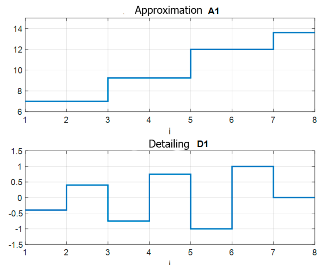
Then, we define the vector f = R * y = [7.0000 0.4000 9.2500 0.7500 12.0000 1.0000 13.6000 0]T which contains the average values of half-sum and half-difference. To calculate the deviations of the elements of groups from the average values, let us form the vector string Fcp = [f(1) f(1) f(3) f(3) f(5) f(5) f(7) f(7)]. The Fcp vector, according to the indications, consists of pairwise arranged average values (half-sum) located in the composition of the elements of the f vector string. Then, we define the deviations of the y vector elements from the average values:
It should be noted that Fcp and R vectors can also be obtained by applying the Haar wavelet transform. To carry out the one-step signal decomposition on the ‘db1’ wavelet basis, we will use the following operators of Wavelet ToolBox:
[cA1,cD1] = dwt (y,‘db1’),
- 2.
The transform A1 = upcoef(‘a’,cA1,‘db1’,1,ls); D1 = upcoef(‘d’,cD1,‘db1’,1,ls).
The upcoef function provides an approximation of A1 and detail D1 of the first wavelet transform level by vectors cA1 and cD1. The adequacy of the estimates is determined by the equalities A1 = Fcp and D1 = r. According to the upcoef syntax, there are symbols ‘a’ and ‘d’, indicating which kind of decomposition should be performed. For approximation, respectively, the vector cA1 is introduced, and for detailing—cD1. Then, the Daubechies wavelet with the number ‘db1’ is selected; the number of the level of operations is entered, for example, 1. The number of elements of the vector of the processed signal ls is also indicated (for the
y vector this value is equal to ls = 8). For this example, the operator [cA1, cD1] = dwt (y, ‘db1’) performs a linear transformation on each group consisting of two elements of the y vector. The rotation matrix M1 is introduced, consisting of the following elements:
which is converted to the form
4. Conversion of Mathematical Models of Components
In this case, the properties of rotation of vectors are preserved with the determinant det (M) = −1, and the matrix itself becomes suitable for performing simple operations on the estimation of cA1 and cD1. As a result, element-by-element for four groups we have:
[cA11_cD11] = M * [y(1) y(2)]’ = [9.8995 − 0.5657]’;
[cA12_cD12] = M * [y(3) y(4)]’ = [13.0815 − 1.0607]’;
[cA13_cD13] = M * [y(5) y(6)]’ = [16.9706 − 1.4142]’;
[cA14_cD14] = M * [y(7) y(8)]’ = [19.2333 0]’.
It can be seen that M matrix is used to normalize the Haar transform, since the determinant of the matrix det(M) is equal to 1.0000. Therefore, when the pair of numbers is rotated, the area of the normalized object does not change, i.e., information is not lost. The lack of information loss allows the vector to be handled in formed pairs of numbers independently. In the Matlab environment, such a transformation is carried out using a block matrix. It consists of blocks M in the main diagonal. Such a matrix can be obtained by element-by-element multiplication R to sqrt (2):
where the element-by-element multiplication is designated in the MATLAB as ‘*’. Note that det(R) = 0.0625 with the determinant of each block 8 * det(R) = 0.5, while
Rows of the M matrix possess orthogonality properties.
If we introduce m1 = M(1,:) and m2 = M(2,:), we obtain the fulfillment of the orthogonality conditions: m1 * m1T = 1,m2 * m2T = 1 иm1 * m2T = 0.m2 * m1T = 0.
An orthogonal matrix inv(W) = WT and the calculation of the return matrix is significantly simplified.
The vector of coefficients A1 and D1, obtained during the Haar transform, are two filters separating the signal to the low-frequency and high-frequency components (
Figure 1). Low-frequency resolution characterizes the signal energy, and the high-frequency one characterizes its frequency associated with short pulses (splashes) and signals with sudden changes.
Now we will restore vector y. The signal regeneration we perform using the inversion of wavelet transform:
With an increase in the amount of the process digitalization by switching to multi-level processing of ECG signals and its individual fragments based on the ‘db1’ wavelet, there is an increase in the transformation quality. It is important for estimating the instantaneous power and the energy of complex short-term pulses [
5,
6,
7,
8,
9]. To be accurate, we will perform a decomposition
y at the level of the detail 3. At this level of detail, we will get C and L:
[C, L] = wavedec(y, 3,‘db1’)
C = [29.5924 − 6.6114 − 2.2500 − 1.6000 − 0.5657 − 1.0607 − 1.4142 0.0000];
L = [1 1 2 4 8].
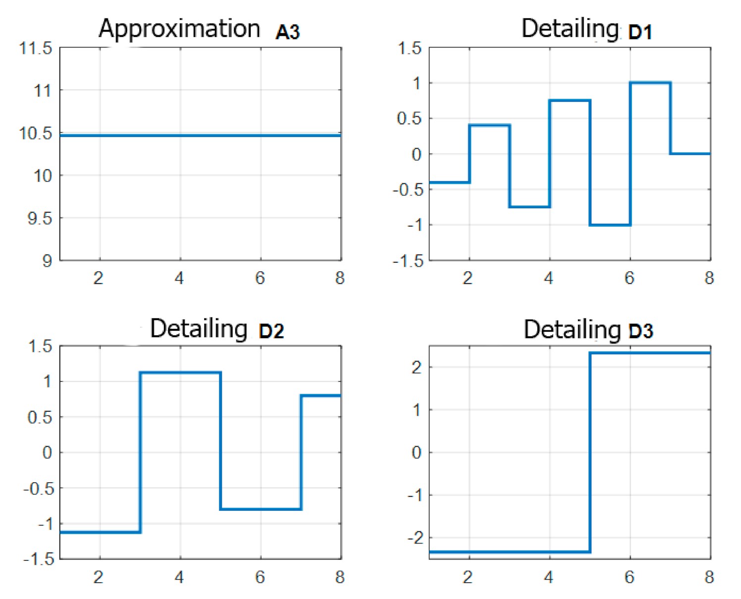
According to the C and L vectors, using the wrcoeff function, we will perform an assessment of the coefficients of the third level of approximation and the detail coefficients of the three levels. Additionally, we will have:
A3 = wrcoef(‘a’,C,L,‘db1’,3);
A3 = [10.4625 10.4625 10.4625 10.4625 10.4625 10.4625 10.4625 10.4625];
D1 = wrcoef(‘d’,C,L,‘db1’,1);
D1 = [−0.4000 0.4000 − 0.7500 0.7500 − 1.0000 1.0000 0.0000 0.0000];
D2 = wrcoef(‘d’,C,L,‘db1’,2);
D2 = [−1.1250 − 1.1250 1.1250 1.1250 − 0.8000 − 0.8000 0.8000 0.8000];
D3 = wrcoef(‘d’,C,L,‘db1’,3);
D3 = [−2.3375 − 2.3375 − 2.3375 − 2.3375 2.3375 2.3375 2.3375 2.3375].
The results of the calculations can be seen in
Figure 2.
The Daubechies wavelets of the ‘db2’ through to ‘db10’ family contained in the Wavelet Toolbox are structured by other principles for the formation of groups of number sequences. Instead of groups of two points, for example, four points are taken with displacement of the elements of the subsequent group at each step into two elements to the left, which significantly improves the process of converting signals. With reference to the vector with dimension (1 × 8), such groups can be represented by the following vectors:
When building low-frequency and high-frequency filters, each group of four numbers will be replaced by two numbers.
The values of the elements of the y vector in the group are equal to x, v, z, t. Then, the first ‘a’ filter is written in the form of the following relation:
Second d filter is represented as a linear model
Such permutation of elements is used to ensure the property of the orthogonality of the Daubechies transform block and is represented as:
To calculate the numerical values of the DB matrix elements, it is necessary to have four equations. The first equation can be determined by the requirement of orthogonality:
and it must be executed for all pairs of rows. Other three equations are drawn up taking into account the requirements defined by the Daubechies transform itself:
- 2.
The equation must take zero values for any identical ‘k’, for example, if k = 1,
- 3.
The transform must also take zero values for linearly increasing elements m, for example, if m = [1 2 3 4],
The system of nonlinear Equations (2)–(5) can be solved only by numerical methods. We use the fsolve function in the MATLAB Optimization Toolbox. Observing the requirements of the function syntax, we present a fragment of the solution. For this purpose, we introduce the formula:
x(1) = c1, x(2) = c2, x(3) = c3, x(4) = c4.
Then, we compose a file function sah568hh.m, where we write Equations (2)–(5) in matrix form:
function F = sah568hh (x);
F = [x(1)^2 + x(2)^2 + x(3)^2 + x(4)^2−1;x(1)*x(3) + x(2)*x(4);−x(1) + x(2)−x(3) + x(4);
−4*x(1) + 3*x(2)−2*x(3) + x(4)];
The iterative process continues until the rows of the matrix F are ‘zeroed’, and in the case of quadratic nonlinearity, the convergence of the solution is guaranteed. Linking to the file function at each iteration is made from the main file sah568h.m,. The file fragment contains the initial approximation vector x0, options for displaying the solution and the fsolve function (
Table 1). At the end of the iterative process, the vector x and the error estimate fval are displayed:
% sah568h.m
x0 = [0.4 0.3 7.0 0.1];
options = optimset(‘Display’,’iter’);
[x,fval] = fsolve(‘sah568hh’,x0,options)
Iterative process:
Equation solved.
Output:
Substituting the numerical values of the x vector elements into Equation (1), we obtain the determinant of the Daubechies matrix equal to det(DB) = 1.0000, as well as the condition DB−1 = DBT, which indicates that the solutions are correct.
Having considered the technology of structuring the Daubechies matrix by example, we can offer an algorithm for processing signals of high dimension. This will ensure the storage of information about the parameters of the individual settings of the pacemaker (ECS) at each scheduled visit to the cardiologist starting from the moment of programming during implantation; this can allow informed decisions to be made about changing the functional mode of the device, taking into account fluctuations of the ECG signal in time.
The use of the algorithm for ECG processing and parametric adjustment of the pacemaker is aimed at expanding the capabilities of the doctor and medical staff in the application of digital technologies in the field of cardiology.
Unlike existing solutions, cardiosignals in the proposed algorithm (initial data) are processed using splines. Interpolation of cardiac signals using cubic splines makes it possible to obtain interpolation nodes on a temporal grid with a variable quantization step, where the step and the number of interpolation nodes are selected depending on the waveform at the appropriate time intervals. Plotting a cubic spline is using the spline function provided in MATLAB tools.
The construction of Daubechies wavelets is performed according to a cascade algorithm, which enables the calculation of the element-by-element scaling function with the allocation of local features of the approximated ECG signals. With a high dimension of the vectors of the analyzed signals, it is advisable to perform wavelet transforms according to the following algorithm:
Input of initial data.
Spline approximation of the input signal.
Selecting a wavelet and assigning a wavelet-decomposition level.
Signal decomposition: determination of approximating and detailing components.
Performing the inversion operation (inverse wavelet transform) to restore the signal.
Estimation of the first level approximation error.
Performing multilevel wavelet decomposition.
Reconstruction of the approximation of the third level and details of 1, 2 and 3 levels.
Graphic interpretation and analysis of the transformation results.
According to the algorithm, we will perform a wavelet analysis of the V2 electrocardiosignal on the GE 1200 ST scale at an HR of 65 bpm, obtained after implantation of a pacemaker. We enter the initial data based on discrete measurements of the intracardiac endogram (on the cellular scale of the information source), from which we form a vector of interpolation nodes on an uneven grid with the subsequent construction of a cubic spline used for wavelet analysis.
Analysis and synthesis were performed using the sah1041c.m file in MATLAB codes. The file is compiled according to the given algorithm and contains comments on its implementation. The data of the ECG signal after appropriate processing are represented by a matrix of Z dimensions (140 × 2). An increase in the accuracy of the experimental data input is provided by the use of splines with a variable step of discreteness, depending on the shape of the signal at the corresponding time interval. By specifying the spline with a matrix of dimension (n × 2), where n = 500, a vector is generated to be digitally processed.
5. Listing the Program in Matlab
% sah1041c.m. Wavelets for electrocardiogram approximation.
%========================================================
% 1. Input of initial data (source: sah1041a.m).
load V2
X = V2(:,1);
Y = V2(:,2);
pause
X1 = X;
Y1 = Y;
% 2. Spline approximation of the input signal.
n = 500;
x = linspace(X1(1),X1(end),n);
y = spline (X1,Y1,x);
x1 = 1:n;
% Scaling y vector (1 × 500)
P = y*4.78 × 10⁻⁵;
v = size(P);
s = P(1:v(2));
l_s= length(s);
% 3. Selecting a wavelet and assigning a wavelet decomposition level.
% Level 1, Daubechies wavelet ‘db1’. Transformation Algorithm Sm1 = A1 + D1
[cA1,cD1] = dwt(s,‘db1’);
%4. Signal decomposition: determination of the approximating
% and detailing components.
A1 = upcoef(‘a’,cA1,‘db1’,1,l_s);
D1 = upcoef(‘d’,cD1,‘db1’,1,l_s);
% 5. Performing an inversion operation (inverse wavelet transform) to restore the signal.
% %
Sm1 = idwt(cA1,cD1,‘db1’,l_s);
% 6. Estimation of the first-level approximation error
err = max(abs(s-Sm1));
% err = 5.4210 × 10⁻¹⁹
% 7. Performing multilevel wavelet decomposition
[C,L] = wavedec(s,3,‘db1’);
cA3 = appcoef(C,L,‘db1’,3);
cD3 = detcoef(C,L,3);
cD2 = detcoef(C,L,2);
cD1 = detcoef(C,L,1);
[cD1,cD2,cD3] = detcoef(C,L,[1−3]);
% 8. Reconstruction of the third level approximation and of details of 1, 2 and 3 levels
%. % 8.
%.
A3 = wrcoef(‘a’,C,L,‘db1’,3);
D1 = wrcoef(‘d’,C,L,‘db1’,1);
D2 = wrcoef(‘d’,C,L,‘db1’,2);
D3 = wrcoef(‘d’,C,L,‘db1’,3);
Sm3 = waverec(C,L,‘db1’);
% Estimation of the error of the three-level approximation
err = max(abs(s-Sm3))
% Error:
% err = 4.9738 × 10⁻¹⁴.
% 9. Graphic interpretation and analysis of transformation results.
subplot(2,2,1); plot(x1,A3);grid; title(‘Approximation,3’)
subplot(2,2,2); plot(x1,D1);grid; title(‘Detailing,1’)
subplot(2,2,3); plot(x1,D2);grid; title(‘Detailing,2’)
subplot(2,2,4); plot(x1,D3);grid; title(‘Detailing,3’)
pause
% Voltage V2 (in volts) at HR 65 bpm.
[thr,sorh,keepapp] = ddencmp(‘den’,‘wv’,s);
Sm = wdencmp(‘gbl’,C,L,‘db1’,3,thr,sorh,keepapp);
subplot(2,1,1); plot(x1*0.0055,P),grid; title(‘Original’);
xlabel(‘Time, s.’);
ylabel(‘Voltage, V.’);
axis([0 2.75 −1 × 10⁻³ 1 × 10⁻³])
subplot(2,1,2); plot(x1*0.0055,Sm),grid; title(‘wavelet-model)
axis([0 2.75 −1 × 10⁻³ 1 × 10⁻³])
xlabel(‘Time, s.’)
ylabel(‘Voltage, V.’)
% Matrix for comparing digital values (on the cellular scale of digitalization) of the spline vector and the reconstructed vector by wavelet transform (dimension (2xn), where n = 500:y_ym = [y;Sm1./4.78 × 10−5];
Implementation of a software component for calculating a process. With a three-step approximation according to the scheme:
The maximum error was estimated using the formula: err = max (abs (s-Sm3)) = 5.4210 × 10⁻¹⁹.
The graphs of the coefficients for the three-level decomposition are shown in
Figure 3.
6. Discussion for Wavelets
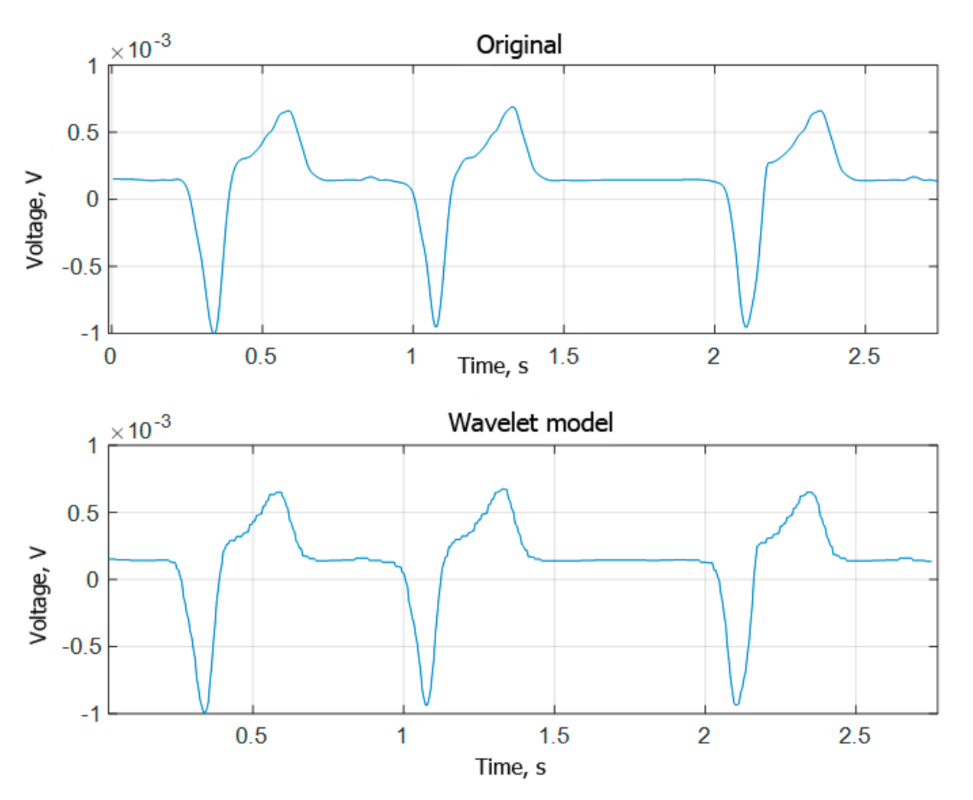
The inverse wavelet transform is implemented using the signal reconstruction functions provided in the file.
Figure 4 shows the original and reconstructed signal characteristics. The identity of the original and reconstructed ECG signals can be verified by the equality of the elements of the columns of the y_ym matrix contained in the file.
Wavelets are widely used in various areas of professional activity in cardiology. Wavelets are used to create mechanisms for processing signals, monitoring the parameters of the cardiosystem condition, diagnosis of diseases, and the adoption of operational solutions using the most complete information about the patient’s health status, etc.
Wavelets are a special class of functions with orthogonal properties and are capable of performing shift and scaling operations (stretch/compression). Any wavelet generates a complete orthogonal system of functions. The Haar and Daubechies wavelets are the most commonly used. Wavelet analysis of cardios signals makes it possible to estimate the difference in characteristics. With the help of wavelet transform it is possible to restore the process, with an estimate of the error. The method for processing one-dimensional signals using the Haar and Daubechies wavelets is considered. It is also necessary to develop new methods and means of reliable early diagnosis of heart conditions on the basis of modern methods of processing and integrated analysis of biomedical signals, which should be the subject of further research.
7. Conclusions
1. Wavelet transform of one-dimensional discrete signals based on the Haar and Daubechies wavelets consist of determining the parameters of low-frequency and high-frequency filters by expanding the basis, designed using the model of the selected wavelet. Each of the functions of the base characterizes its spatial (time) frequency and localization in space.
2. For the measurement vector consisting of eight ECG signal elements, a method of separation into groups has been proposed. It makes it possible to get the Daubechies matrix (8 × 8). The determinant of the matrix is equal to one. Orthogonal properties are used to replace the inversion operation of the Daubechies matrix transposition operation.
3. The elements of the Daubechies matrix are defined by the numerical solution of the system of nonlinear equations in the MATLAB environment. A file function is compiled, which admits the iterative process of ‘zeroing’ the rows of the matrix under the conditions of orthogonality and the constancy of the determinant.
4. Calculations are made on the basis of Wavelet ToolBox package functions that confirmed the correctness of transformations and solutions in the decomposition and synthesis of the original function.
5. The algorithm for working with one-dimensional discrete signals and high-dimension vectors is given. It is used for the ECG wavelet transform with the introduction of interpolation nodes on a non-uniform grid and the use of spline approximation. The signal is restored according to the components of the three-level approximation of A3 and the D1, D2, and D3 details.
6. It is shown that in order to improve the efficiency of working with wavelet transforms, the specifics of working with certain objects should be taken into account.
7. The main task of wavelet analysis when diagnosing is to establish a correspondence between the coefficients of the decomposition and the ‘standard’ forms of ECG signals with the regulatory criteria for the assessment.
8. Development and application of wavelet analysis in cardiology are important tools for the digitalization of complex prospective technologies to maintain people’s health throughout their lives.


