Cyclic Detectors in the Fraction-of-Time Probability Framework

Abstract

The signal detection problem for cyclostationary signals is addressed within the fraction-of-time probability framework, where statistical functions are constructed starting from a single time series, without introducing the concept of stochastic process. Single-cycle detectors and quadratic-form detectors based on measurements of the Fourier coefficients of the almost-periodically time-variant cumulative distribution and probability density functions are proposed. The adopted fraction-of-time approach provides both methodological and implementation advantages for the proposed detectors. For single-cycle detectors, the decision statistic is a function of the received signal and the threshold is derived using side data under the null hypothesis. For quadratic-form detectors, the decision statistic can be expressed as a function of the received signal without using side data, at the cost of some performance degradation. The threshold can be derived analytically. Performance analysis is carried out using Monte Carlo simulations in severe noise and interference environments, where the proposed detectors provide better performance with respect to the analogous detectors based on second- and higher-order cyclic statistic measurements.

1. Introduction

Cyclostationarity is a property exhibited by almost all modulated signals adopted in communications, radar/sonar, and telemetry [1,2]. Cyclostationary signals exhibit statistical functions, such as the cumulative distribution, probability density, autocorrelation, moments, and cumulants that are periodic functions of time. More generally, these statistical functions can be almost periodic [3]; that is, they can be expressed by the superposition of sine waves with possibly incommensurate frequencies. In such a case, the signals are referred to as almost cyclostationary (ACS). The statistical properties of ACS signals are suitably described by the Fourier coefficients, referred to as cyclic statistics, of these almost-periodic functions. The frequencies of the (generalized) Fourier series expansions are related to signal parameters such as the carrier frequency, baud rate, and sampling or scanning frequency. Thus, the frequencies of the harmonics, referred to as cycle frequencies, are a characteristic of a signal. In particular, signals having different abovementioned parameters exhibit different cycle frequencies. This fact has been exploited for the design of detection and estimation algorithms that are signal selective. In fact, in the presence of a mixture of signal of interest (SOI) and disturbance, characteristics of the SOI alone can be estimated, provided that a cycle frequency of the SOI exists, which is not shared with the disturbance signal, regardless of the temporal and spectral overlap of the SOI and disturbance [1] (Chapter 14), [2] (Section 9.2).

Several cyclostationarity-based detectors have been presented in the literature. Single-cycle and multi-cycle detectors are proposed in [4,5,6], with reference to second-order statistics, and in [7], with reference to higher-order statistics. A statistical test for the presence of cyclostationarity is proposed in [8] and its application to signal detection is discussed in [2] (Section 8.4), [9]. A statistical test for the presence of spectral coherence is proposed in [10]. Spectral coherence is also exploited in [11,12]. Detection strategies based on the estimated confidence interval of estimated cyclic statistics are presented in [2] (Section 8.7). They are based on the results in [13]. Applications to cognitive radio are presented in [14,15,16,17,18]. The case of an unknown cyclostationarity period is addressed in [19,20]. The case of irregular cyclicity is treated in [21,22,23,24].

All the of abovementioned cyclostationarity-based detectors exploit measurements of second- or higher-order cyclic statistics. In this paper, a new class of cyclic detectors is proposed. Specifically, detectors based on measurements of the Fourier coefficients of the almost-periodically time-variant cumulative distribution function (CDF) and probability density function (pdf) are introduced. Numerical results presented here show that performance gains can be obtained by constructing cyclostationarity-based detectors that exploit these cyclic statistical functions.

In practical detection problems, a single realization of the received signal is available and a decision on the hypothesis “SOI not present” (null hypothesis) or “SOI present” (alternative hypothesis) must be taken on the basis of this unique observed signal. That is, no ensemble of realizations is available for making the decision. For this reason, in this paper, the statistical characterization of the received signal and of its cyclic statistical function measurements is made using the fraction-of-time (FOT) probability approach. In such an approach, a signal is modeled as a single function of time, rather than a realization of a stochastic process [1,25,26,27,28]. Then, statistical functions such as distribution, autocorrelation, moments, and cumulants are constructed, starting from this unique function of time. This approach has the methodological advantage that the statistical characterization of the measurements of the cyclic statistical functions of the received signal can be performed without resorting to any abstract stochastic process. The advantage is not only methodological but also in the detector implementation. In fact, a class of detectors is presented here such that the decision statistic is derived exclusively from the received signal, with no aid from side data under the null hypothesis, and the threshold is analytically determined.

Two classes of cyclostationarity-based detectors are considered: single-cycle (SC) detectors, and quadratic-form (QF) detectors. For each class, the decision statistic is constructed using measurements of the Fourier coefficients of the almost-periodically time-variant CDF and pdf. Moreover, for comparison purposes, analogous detectors based on measurements of second- and higher-order cyclic statistic are also considered.

Performance analysis in a very severe noise and interference environment is carried out via Monte Carlo simulations.

The novel contributions of this paper are (i) the proposal of new cyclostationarity-based detection tests that exploit the almost-periodicity of the first-order FOT CDF and pdf; (ii) the proposal of new kernel-based cyclic CDF and pdf estimators; (iii) the exploitation of the FOT approach to statistically characterize the decision statistic, in order to analytically derive the detection threshold; and (iv) the presentation of the cyclostationarity-based detectors in a unified framework that accommodates both existing and new detectors.

The paper is organized as follows: The materials and methods are presented in Section 2. Specifically, in Section 2.1, the signal decomposition into an almost-periodic component and a residual term is considered; in Section 2.2, the definitions and notation for signal analysis in the FOT approach for almost-cyclostationary signals are briefly reviewed. In Section 2.3, estimators for FOT cyclic statistical functions are presented. Specifically, the estimator for the cyclic CDF (Section 2.3.1), the new proposed kernel-based estimators for the cyclic CDF and pdf (Section 2.3.2), estimators for cyclic autocorrelation (Section 2.3.3), the cyclic spectrum (Section 2.3.4), and the 4th-order cyclic moment (Section 2.3.5) are considered. The detection problem is stated in Section 2.4 and cyclostationarity-based detectors are presented in a unified general formalism that accommodates several detection strategies. Single-cycle detectors are treated in Section 2.5, and quadratic-form detectors in Section 2.6. QF detectors based on measurements of the cyclic autocorrelation, spectrum, and moment are addressed in Section 2.6.1. A new class of QF detectors based on measurements of the cyclic CDF and pdf is presented in Section 2.6.2. For QF detectors, the detector structure is presented in Section 2.6.3. A statistical test for the presence of cyclostationarity is described in Section 2.6.4. The numerical results are reported in Section 3. The simulation setup is described in Section 3.1. The cases of threshold determined using Monte Carlo simulation and of analytically derived threshold are treated in Section 3.2 and Section 3.3, respectively. Performance analysis is carried out in Section 3.4, in terms of the probability of missed detection versus data-record length, and in Section 3.5 and Section 3.6, in terms of the receiver operating characteristic (ROC). For the QF detectors, the match or mismatch between the Monte Carlo probability of false alarm and the nominal or design probability of false alarm is analyzed in Section 3.7. A conclusive discussion is given in Section 4.

2. Materials and Methods

2.1. Signal Decomposition

Let us denote by

$${〈z\left(t\right)〉}_t\triangleq \underset{T\to \infty }{lim}\frac{1}{T}{\int }_{t_0-T/2}^{t_0+T/2}z\left(t\right)\mathrm{d}t$$

(1)

the continuous-time infinite-time average of the signal $z\left(t\right)$, provided that the limit in the right-hand side exists. When such a limit exists, it does not depend on $t_0$. In notation ${\langle ·\rangle }_t$, subscript t emphasizes that the average is made with respect to t.

A signal $z\left(t\right)$ can be decomposed into its almost-periodic component $z_{\mathrm{ap}}\left(t\right)$ and a residual term $z_{\mathrm{r}}\left(t\right)$ not containing any finite-strength additive sine-wave component [2] (Section 2.3.1)

$$z\left(t\right)=z_{\mathrm{ap}}\left(t\right)+z_{\mathrm{r}}\left(t\right)$$

(2)

where

$$z_{\mathrm{ap}}\left(t\right)={\displaystyle \sum _{\alpha \in \mathrm{A}}}{z}^{\alpha }{e}^{j2\pi \alpha t}$$

(3)

is the (generalized) Fourier series of the almost-periodic component whose convergence can be uniform, or in a generalized sense [2] (Appendix B.4), [3] (Chapter 2),

$$z^{\alpha }={〈z_{\mathrm{ap}}\left(t\right)e^{-j2\pi \alpha t}〉}_t={〈z\left(t\right)e^{-j2\pi \alpha t}〉}_t\forall \alpha \in \mathrm{A}$$

(4)

are the Fourier coefficients, and

$${〈z_{\mathrm{r}}\left(t\right)e^{-j2\pi \alpha t}〉}_t=0\forall \alpha \in \mathbb{R}$$

(5)

is the residual term. In (3), $\mathrm{A}$ is a countable set of possibly incommensurate frequencies.

The almost-periodic component extraction operator is defined as [2] (Definition 2.14)

$${\mathrm{E}}^{\left\{\alpha \right\}}\left\{z\left(t\right)\right\}\triangleq z_{\mathrm{ap}}\left(t\right)$$

(6)

that is, the operator ${\mathrm{E}}^{\left\{\alpha \right\}}\{·\}$ extracts all the finite-strength additive sine-wave components of its argument. This turns out to be the expectation operator in the FOT probability framework.

2.2. Fraction-of-Time Probability

In this section, a brief review of the FOT approach is provided, in order to introduce the essential definitions and notation. In the FOT approach, signals are modeled as single functions of time rather than as realizations of an ensemble of functions, namely a stochastic process. All time-invariant statistical functions such as the distribution, autocorrelation, moments, and cumulants can be constructed starting from the unique available signal by resorting to the concept of relative measure [29,30], which plays a role analogous to the probability measure in the classical stochastic approach [25]. In such a case, the infinite-time average turns out to be the expectation operator that allows one to construct time-invariant statistical functions. The time-invariant FOT approach can be extended to accommodate periodically or almost-periodically time-variant statistical functions, in order to provide a suitable FOT probabilistic description for time series that exhibit cyclostationarity. In such a case, the expectation operator is the almost-periodic component extraction operator (6). For comprehensive treatments, see [1], [2] (Chapter 2), [31,32]. For extensions, see [33,34].

Let $x\left(t\right)$ be a continuous-time real-valued signal. The almost-periodic FOT cumulative distribution function (CDF) of $x\left(t\right)$ is defined as [2] (Equation (2.33))

$$\begin{array}{cc}\hfill F_x^{\left\{\alpha \right\}}(\xi ;t)\triangleq & {\mathrm{E}}^{\left\{\alpha \right\}}\left\{\mathrm{u}(\xi -x\left(t\right))\right\}\hfill \end{array}$$

(7a)

$$\begin{array}{cc}\hfill =& {\displaystyle \sum _{\gamma \in {\mathrm{\Gamma }}_1}}{F}_x^{\gamma }\left(\xi \right)e^{j2\pi \gamma t}\hfill \end{array}$$

(7b)

where

$$\mathrm{u}\left(\xi \right)\triangleq \left\{\begin{array}{cc}1\hfill & \xi ⩾0\hfill \\ 0\hfill & \xi <0\hfill \end{array}\right.$$

(8)

is the unit-step function, ${\mathrm{\Gamma }}_1$ is a countable set of possibly incommensurate cycle frequencies, and the Fourier coefficients [2] (Equation (2.34))

$$F_x^{\gamma }\left(\xi \right)\triangleq {〈\mathrm{u}(\xi -x\left(t\right))e^{-j2\pi \gamma t}〉}_t\gamma \in {\mathrm{\Gamma }}_1$$

(9)

are referred to as cyclic CDFs.

If the CDF is differentiable with respect to $\xi$, the almost-periodic FOT probability density function (pdf) of the real-valued signal $x\left(t\right)$ can be defined. This can be formally expressed (in the sense of generalized functions [35]) as [2] (Equation (2.37))

$$\begin{array}{cc}\hfill f_x^{\left\{\alpha \right\}}(\xi ;t)\triangleq & \frac{\mathrm{d}}{\mathrm{d}\xi }{F}_x^{\left\{\alpha \right\}}(\xi ;t)\hfill \end{array}$$

(10a)

$$\begin{array}{cc}\hfill =& {\mathrm{E}}^{\left\{\alpha \right\}}\left\{\delta (\xi -x\left(t\right))\right\}\hfill \end{array}$$

(10b)

$$\begin{array}{cc}\hfill =& {\displaystyle \sum _{\gamma \in {\mathrm{\Gamma }}_1}}{f}_x^{\gamma }\left(\xi \right)e^{j2\pi \gamma t}\hfill \end{array}$$

(10c)

where the Fourier coefficients are formally expressed as

$$\begin{array}{cc}\hfill f_x^{\gamma }\left(\xi \right)\triangleq & {〈\delta (\xi -x\left(t\right))e^{-j2\pi \gamma t}〉}_t\hfill \end{array}$$

(11a)

$$\begin{array}{cc}\hfill =& \frac{\mathrm{d}}{\mathrm{d}\xi }{F}_x^{\gamma }\left(\xi \right)\gamma \in {\mathrm{\Gamma }}_1\hfill \end{array}$$

(11b)

and are referred to as cyclic pdfs. In (10b) and (11a), $\delta (·)$ denotes Dirac delta.

The following fundamental theorem of expectation holds [31]:

$$\begin{array}{cc}\hfill {\mathrm{E}}^{\left\{\alpha \right\}}\left\{x\left(t\right)\right\}\triangleq & {\int }_{\mathbb{R}}\xi \mathrm{d}{F}_x^{\left\{\alpha \right\}}(\xi ;t)\hfill \end{array}$$

(12a)

$$\begin{array}{cc}\hfill =& {\int }_{\mathbb{R}}\xi f_x^{\left\{\alpha \right\}}(\xi ;t)\mathrm{d}\xi \hfill \end{array}$$

(12b)

$$\begin{array}{cc}\hfill =& {\displaystyle \sum _{\eta \in {\mathrm{A}}_1}}{x}^{\eta }{e}^{j2\pi \eta t}\hfill \end{array}$$

(12c)

where the Fourier coefficients of the almost-periodic component of $x\left(t\right)$ can be expressed as

$$\begin{array}{cc}\hfill x^{\eta }\triangleq & {〈x\left(t\right)e^{-j2\pi \eta t}〉}_t\hfill \end{array}$$

(13a)

$$\begin{array}{cc}\hfill =& {\int }_{\mathbb{R}}\xi \mathrm{d}{F}_x^{\eta }\left(\xi \right)\hfill \end{array}$$

(13b)

$$\begin{array}{cc}\hfill =& {\int }_{\mathbb{R}}\xi f_x^{\eta }\left(\xi \right)\mathrm{d}\xi \eta \in A_1\hfill \end{array}$$

(13c)

with

$${\mathrm{A}}_1\subseteq {\mathrm{\Gamma }}_1$$

(14)

The function defined in (12a) is the almost-periodic mean (in the FOT sense) of the signal $x\left(t\right)$ and (12b) is the FOT counterpart of the fundamental theorem of expectation in the stochastic approach. The Fourier coefficients defined in (13a) are referred to as cyclic means.

The second-order characterization of a time series $x\left(t\right)$ is based on the almost-periodic joint FOT CDF of $x(t+\tau )$ and $x\left(t\right)$ [2] (Theorem 2.34), [31]

$$\begin{array}{cc}\hfill F_x^{\left\{\alpha \right\}}({\xi }_1,{\xi }_2;t,\tau )\triangleq & {\mathrm{E}}^{\left\{\alpha \right\}}\left\{\mathrm{u}({\xi }_1-x(t+\tau ))\mathrm{u}({\xi }_2-x\left(t\right))\right\}\hfill \end{array}$$

(15a)

$$\begin{array}{cc}\hfill =& {\displaystyle \sum _{\gamma \in {\mathrm{\Gamma }}_2}}{F}_x^{\gamma }({\xi }_1,{\xi }_2;\tau )e^{j2\pi \gamma t}\hfill \end{array}$$

(15b)

where ${\mathrm{\Gamma }}_2$ is a countable set of possibly incommensurate cycle frequencies, and the Fourier coefficients

$$F_x^{\gamma }({\xi }_1,{\xi }_2;\tau )\triangleq {〈\mathrm{u}({\xi }_1-x(t+\tau ))\mathrm{u}({\xi }_2-x\left(t\right))e^{-j2\pi \gamma t}〉}_t\gamma \in {\mathrm{\Gamma }}_2$$

(16)

are referred to as cyclic joint CDFs.

If the joint FOT CDF is differentiable with respect to both ${\xi }_1$ and ${\xi }_2$, the almost-periodic joint FOT pdf of $x(t+\tau )$ and $x\left(t\right)$ can be defined. This can be formally expressed as [2] (Equation (2.50))

$$\begin{array}{cc}\hfill f_x^{\left\{\alpha \right\}}({\xi }_1,{\xi }_2;t,\tau )\triangleq & \frac{{\partial }^2}{\partial {\xi }_1\partial {\xi }_2}{F}_x^{\left\{\alpha \right\}}({\xi }_1,{\xi }_2;t,\tau )\hfill \end{array}$$

(17a)

$$\begin{array}{cc}\hfill =& {\mathrm{E}}^{\left\{\alpha \right\}}\left\{\delta ({\xi }_1-x(t+\tau ))\delta ({\xi }_2-x\left(t\right))\right\}\hfill \end{array}$$

(17b)

$$\begin{array}{cc}\hfill =& {\displaystyle \sum _{\gamma \in {\mathrm{\Gamma }}_2}}{f}_x^{\gamma }({\xi }_1,{\xi }_2;\tau )e^{j2\pi \gamma t}\hfill \end{array}$$

(17c)

where the Fourier coefficients

$$\begin{array}{cc}\hfill f_x^{\gamma }({\xi }_1,{\xi }_2;\tau )\triangleq & {〈\delta ({\xi }_1-x(t+\tau ))\delta ({\xi }_2-x\left(t\right))e^{-j2\pi \gamma t}〉}_t\hfill \end{array}$$

(18a)

$$\begin{array}{cc}\hfill =& \frac{{\partial }^2}{\partial {\xi }_1\partial {\xi }_2}{F}_x^{\gamma }({\xi }_1,{\xi }_2;\tau )\gamma \in {\mathrm{\Gamma }}_2\hfill \end{array}$$

(18b)

are referred to as cyclic joint pdfs.

The following fundamental theorem of expectation holds [2] (Theorem 2.35), [31]:

$$\begin{array}{cc}\hfill {\mathrm{E}}^{\left\{\alpha \right\}}\left\{x(t+\tau )x\left(t\right)\right\}=& {\int }_{\mathbb{R}}{\xi }_1{\xi }_2\mathrm{d}{F}_x^{\left\{\alpha \right\}}({\xi }_1,{\xi }_2;t,\tau )\hfill \end{array}$$

(19a)

$$\begin{array}{cc}\hfill =& {\int }_{\mathbb{R}}{\xi }_1{\xi }_2{f}_x^{\left\{\alpha \right\}}({\xi }_1,{\xi }_2;t,\tau )\mathrm{d}{\xi }_1\mathrm{d}{\xi }_2\hfill \end{array}$$

(19b)

$$\begin{array}{cc}\hfill =& {\displaystyle \sum _{\alpha \in {\mathrm{A}}_2}}{R}_x^{\alpha }\left(\tau \right)e^{j2\pi \alpha t}\hfill \end{array}$$

(19c)

where the function ${\mathrm{E}}^{\left\{\alpha \right\}}\left\{x(t+\tau )x\left(t\right)\right\}$ has all the properties of an autocorrelation function and the Fourier coefficient

$$\begin{array}{cc}\hfill R_x^{\alpha }\left(\tau \right)\triangleq & {〈x(t+\tau )x\left(t\right)e^{-j2\pi \alpha t}〉}_t\hfill \end{array}$$

(20a)

$$\begin{array}{cc}\hfill =& {\int }_{\mathbb{R}}{\xi }_1{\xi }_2\mathrm{d}{F}_x^{\alpha }({\xi }_1,{\xi }_2;\tau )\hfill \end{array}$$

(20b)

$$\begin{array}{cc}\hfill =& {\int }_{\mathbb{R}}{\xi }_1{\xi }_2{f}_x^{\alpha }({\xi }_1,{\xi }_2;\tau )\mathrm{d}{\xi }_1\mathrm{d}{\xi }_2\hfill \end{array}$$

(20c)

is referred to as cyclic autocorrelation function at cycle frequency $\alpha$. It results that

$${\mathrm{A}}_2\subseteq {\mathrm{\Gamma }}_2.$$

(21)

The second-order characterization of a time series $x\left(t\right)$ in the spectral domain is made in terms of the cyclic spectrum $S_x^{\alpha }\left(f\right)$. This is defined as the correlation between the spectral components of the signal at frequencies f and $f-\alpha$, where $\alpha \in {\mathrm{A}}_2$ is one of the cycle frequencies of the signal $x\left(t\right)$ [1] (Chapter 11), [2] (Chapter 2). For this reason, $S_x^{\alpha }\left(f\right)$ is also referred to as spectral correlation density. It is linked to the cyclic autocorrelation by Gardner’s relation [2] (Section 2.3.1.10)

$$S_x^{\alpha }\left(f\right)={\int }_{\mathbb{R}}{R}_x^{\alpha }\left(\tau \right)e^{-j2\pi f\tau }\mathrm{d}\tau$$

(22)

also referred to as the cyclic Wiener–Khinchin relation.

Higher-order statistics of almost-cyclostationary signals in the FOT probability framework were introduced in [7,32]. In this paper, only the 4th-order reduced-dimension cyclic temporal moment function

$$R_x^{\alpha }({\tau }_1,{\tau }_2,{\tau }_3)\triangleq {〈x(t+{\tau }_1)x(t+{\tau }_2)x(t+{\tau }_3)x\left(t\right)e^{-j2\pi \alpha t}〉}_t$$

(23)

referred to as, in short, 4th-order cyclic moment, is considered to build a higher-order cyclostationarity (HOCS)-based detector.

2.3. Cyclic Statistical Functions Estimators

In this section, estimators for the FOT cyclic statistical functions considered in Section 2.2 are presented. These estimators are obtained by considering finite time-averages in place of the infinite-time averages present in the definitions of the FOT statistical functions [1] (Chapter 13), [2,36] (Section 5.6). Moreover, for the cyclic CDF and the cyclic pdf, kernel-based estimators are proposed here for the first time.

In the FOT approach, the randomness (variability) of the estimate depends on the choice of the central point of the finite observation interval (i.e., $t_0$ in (1) with T finite; that is, without the limit operation) [36], [2] (Section 5.6). In the almost-periodic case, one estimates the Fourier coefficients of almost-periodic functions. Thus, $z\left(t\right)$ in (1) is a sinusoidally weighted version of the second-order lag-product $x(t+\tau )x\left(t\right)$ or of the indicator function $\mathrm{u}(\xi -x(t\left)\right)$. Statistical functions of estimates for $t\in [t_0-T/2,t_0+T/2]$ are built considering estimates in smaller observation intervals $[u-b/2,u+b/2]$, with $b\ll T$, and averaging these estimates when u ranges within $[t_0-T/2+b/2,t_0+T/2-b/2]$ [36]. An example is provided in Section 2.6.3.

2.3.1. Cyclic CDF

The natural estimator of the cyclic CDF (9) is

$$F_x^{\left(T\right)}(\gamma ,\xi ;t_0)\triangleq \frac{1}{T}{\int }_{t_0-T/2}^{t_0+T/2}\mathrm{u}(\xi -x\left(t\right))e^{-j2\pi \gamma t}\mathrm{d}t$$

(24)

Under [36] (Assumptions 3.4 and 3.5), with $x\left(t\right)$ replaced by $\mathrm{u}(\xi -x\left(t\right))e^{-j2\pi \gamma t}$, according to [36] (Theorem 3.7), the function in (24) is a mean-square consistent estimator of the Fourier coefficient (9), and the normalized estimation error

$$\sqrt{T}\left[F_x^{\left(T\right)}(\gamma ,\xi ;t_0)-F_x^{\gamma }\left(\xi \right)\right]$$

(25)

is asymptotically $(T\to \infty )$ complex normal.

Note that [36] (Assumptions 3.4 and 3.5), with $x\left(t\right)$ replaced by $\mathrm{u}(\xi -x\left(t\right))e^{-j2\pi \gamma t}$, correspond to assuming asymptotic independence, in the FOT sense, for the signal $x\left(t\right)$.

2.3.2. Cyclic CDF and pdf (Kernel-Based Estimators)

Kernel-based estimators of the cyclic CDF and the cyclic pdf are proposed here for the first time. They are obtained by generalizing the definitions for time-invariant CDF and pdf. However, only early results are so far available for these estimators, and their properties are still under investigation.

The kernel-based estimators of the FOT cyclic pdf (11b) and of the FOT cyclic CDF (9) of a continuous-time signal $x\left(t\right)$ are a generalization of the continuous-time counterparts of the kernel-based estimators of the pdf and CDF proposed for discrete-time processes in [37,38], [39] (Section 2.1.8, pp. 64–65). They are given by

$$f_x^{(T,b_T)}(\gamma ,\xi ;t_0)=\frac{1}{T}{\int }_{t_0-T/2}^{t_0+T/2}\frac{1}{b_T}W\left(\frac{\xi -x\left(t\right)}{b_T}\right)e^{-j2\pi \gamma t}\mathrm{d}t$$

(26)

and

$$\begin{array}{cc}\hfill F_x^{(T,b_T)}(\gamma ,\xi ;t_0)=& {\int }_{-\infty }^{\xi }{f}_x^{(T,b_T)}(\gamma ,s;t_0)\mathrm{d}s\hfill \end{array}$$

(27a)

$$\begin{array}{cc}\hfill =& \frac{1}{T}{\int }_{t_0-T/2}^{t_0+T/2}{W}_c\left(\frac{\xi -x\left(t\right)}{b_T}\right)e^{-j2\pi \gamma t}\mathrm{d}t\hfill \end{array}$$

(27b)

respectively, where $W\left(s\right)$ is a unit-area smoothing window,

$$W_c\left(\xi \right)\triangleq {\int }_{-\infty }^{\xi }W\left(s\right)\mathrm{d}s$$

(28)

and $b_T$ is the smoothing parameter. When $t_0=0$ or the dependence on $t_0$ is not of interest, in the left-hand sides of (26) and (27a) such a dependence is omitted for the sake of brevity.

In the special case $\gamma =0$, the discrete-time counterparts of the estimators (26) and (27b) are characterized in the stochastic approach in [37,38], [39] (Section 2.1.8, pp. 64–65) (in which case, $t_0=0$ and the variability (randomness) of the estimate is considered on the ensemble of realizations of a stochastic process). Specifically, under mild assumptions, $f_x^{(T,b_T)}(0,\xi )$ and $F_x^{(T,b_T)}(0,\xi )$ are shown to be mean-square consistent estimators of the pdf $f_x^0\left(\xi \right)$ and the CDF $F_x^0\left(\xi \right)$, respectively, provided that [38] the following conditions hold:

$$T\to \infty b_T\to 0T{b}_T\to \infty$$

(29)

In addition, for $\gamma =0$, Silverman’s rule of thumb

$$b_T={(4/3)}^{1/5}{\sigma }_x{T}^{-1/5}$$

(30)

where ${\sigma }_x$ is the standard deviation of $x\left(t\right)$, assures the minimum mean-squared error of the CDF and pdf estimates [38] (Equation (20)). Furthermore, for $\gamma =0$, the normalized estimation errors

$$\sqrt{T{b}_T}\left[f_x^{(T,b_T)}(0,\xi )-f_x^0\left(\xi \right)\right]$$

(31)

and

$$\sqrt{T{b}_T}\left[F_x^{(T,b_T)}(0,\xi )-F_x^0\left(\xi \right)\right]$$

(32)

are asymptotically normal, provided that $T{b}_T^3\to \infty$ as $T\to \infty$ [38] (p. 1822). See [40] for the case of continuous-time processes.

Numerical experiments have shown that, for $\gamma \ne 0$, the estimators (26) and (27b) provide reliable estimates (i.e., exhibiting small bias and variance) of the cyclic pdf and the cyclic CDF, respectively, as the data record length T increases and the smoothing parameter $b_T$ decreases. This fact suggests that, under appropriate conditions, the mean-square consistence can be proved. In contrast, the asymptotic normality property does not seem to hold. The plausibility of this conjecture is corroborated by the results presented in Section 3.

An alternative technique for FOT pdf estimation based on linear interpolation of time series is presented in [41].

2.3.3. Cyclic Autocorrelation

The natural estimator of the cyclic autocorrelation Function (20a) is the cyclic correlogram [2] (Definition 5.1)

$$R_x^{\left(T\right)}(\alpha ,\tau ;t_0)\triangleq \frac{1}{T}{\int }_{t_0-T/2}^{t_0+T/2}x(t+\tau )x\left(t\right)e^{-j2\pi \alpha t}\mathrm{d}t$$

(33)

Under mild assumptions, the cyclic correlogram (33) is a mean-square consistent estimator of the cyclic autocorrelation (20a) [2] (Theorem 5.15), [42] and the normalized estimation error

$$\sqrt{T}\left[R_x^{\left(T\right)}(\alpha ,\tau ;t_0)-R_x^{\alpha }\left(\tau \right)\right]$$

(34)

is asymptotically $(T\to \infty )$ complex normal [2] (Theorem 5.18), [43].

The results in [2] (Theorems 5.15 and 5.18) are derived with the classical stochastic approach. Their FOT counterpart can be obtained by using [36] (Theorem 3.7) for the time-average of the function of time

$$t\mapsto x(t+\tau )x\left(t\right)e^{-j2\pi \alpha t}$$

(35)

2.3.4. Cyclic Spectrum

The cyclic spectrum (22) can be consistently estimated using the frequency-smoothed cyclic periodogram [1], [2] (Section 5.2.3), [44] (Chapter 13), [45] (Section 4.6) or with the time-smoothed cyclic periodogram [1] (Chapter 13), [2] (Section 5.2.4), [45] (Section 4.5), [46].

Let $\mathrm{\Delta }f$ be the spectral frequency resolution of the cyclic spectrum estimator. This is coincident with the width of the frequency-smoothing window for the frequency-smoothed cyclic periodogram and with the reciprocal of the block-length for the time-smoothed cyclic periodogram. For both estimators, under mild assumptions, the normalized error estimates are asymptotically ($T\to \infty$) complex normal, provided that $\mathrm{\Delta }f=\mathrm{\Delta }{f}_T\to 0$ and $T\mathrm{\Delta }{f}_T\to \infty$.

2.3.5. 4th-Order Cyclic Moment

The natural estimator of the 4th-order cyclic moment (23) is the 4th-order cyclic correlogram [2] (Definition 5.1)

$$R_x^{\left(T\right)}(\alpha ,{\tau }_1,{\tau }_2,{\tau }_3;t_0)\triangleq \frac{1}{T}{\int }_{t_0-T/2}^{t_0+T/2}x(t+{\tau }_1)x(t+{\tau }_2)x(t+{\tau }_3)x\left(t\right)e^{-j2\pi \alpha t}\mathrm{d}t$$

(36)

Asymptotic results similar to those valid for the cyclic correlogram (33) can be derived [2] (Section 5.7) [7,47,48]. Moreover, their counterpart in the FOT approach can be obtained using [36] (Theorem 3.7).

2.4. Detection

Let us consider the hypothesis test

$$\begin{array}{cc}{\mathrm{H}}_0:& r\left(t\right)=n\left(t\right)\hfill \\ {\mathrm{H}}_1:& r\left(t\right)=x\left(t\right)+n\left(t\right)\hfill \end{array}t\in [-T/2,T/2]$$

(37)

where $x\left(t\right)$ is the signal-of-interest (SOI) and $n\left(t\right)$ is noise.

The detection problem consists in deciding which hypothesis holds true on the basis of the observation of the (unique) received signal $r\left(t\right)$ observed in the finite time interval $t\in [-T/2,T/2]$. If this unique observed signal is modeled as a segment of an infinitely long time series, the natural framework for its statistical characterization is the FOT probability framework.

If the joint FOT probability density functions of $x(t+{\tau }_i)$ and $n(t+{\tau }_i)$ for $t+{\tau }_i\in [0,T]$, $i=1,\cdots ,N$, is unknown or complicated, then the likelihood ratio test (LRT) or the generalized likelihood ratio test (GLRT) cannot be derived. However, sub-optimal receivers can be adopted which use cyclic statistical function measurements as front end data.

In this section, several cyclostationarity-based detectors; that is, that adopt cyclic statistical function measurements as front end data, are presented by a unified notation. Specifically, let us denote by $z_r^{\alpha }\left(\theta \right)$ any of the cyclic statistical functions introduced in Section 2.2. Thus, $\theta$ represents any of the parameters $\tau$, f, or $\xi$. In the case of the 4th-order cyclic moment, $\theta$ is the three-dimensional vector of lags $({\tau }_1,{\tau }_2,{\tau }_3)$. Let ${\widehat{z}}_r(\alpha ,\theta ;t_0)$ be an estimator of $z_r^{\alpha }\left(\theta \right)$ obtained by observing $r\left(t\right)$ for $t\in [t_0-T/2,t_0+T/2]$ (see Section 2.3). In order to simplify the notation, the dependence on $t_0$ in ${\widehat{z}}_r(\alpha ,\theta ;t_0)$ is omitted when unnecessary, if this does not create ambiguity.

As discussed in Section 2.3, under mild assumptions, the normalized estimation error

$${\nu }_T\left[{\widehat{z}}_r(\alpha ,\theta ;t_0)-z_r^{\alpha }\left(\theta \right)\right]$$

(38)

is asymptotically ($T\to \infty$) complex normal. In (38), the normalizing factor ${\nu }_T$ is given by ${\nu }_T=\sqrt{T}$ for the estimators of the cyclic CDF (Section 2.3.1), cyclic autocorrelation (Section 2.3.3), and cyclic 4th-order moment (Section 2.3.5), by ${\nu }_T=\sqrt{T\mathrm{\Delta }{f}_T}$ for the estimators of the cyclic spectrum (Section 2.3.4), and by ${\nu }_T=\sqrt{T{b}_T}$ for the kernel-based estimators of the cyclic CDF and pdf with $\gamma =0$ (Section 2.3.2). Furthermore, the normalized estimation errors

$${\nu }_T\left[{\widehat{z}}_r({\alpha }_k,{\theta }_k;t_0)-z_r^{{\alpha }_k}\left({\theta }_k\right)\right]$$

(39)

at pairs $({\alpha }_k,{\theta }_k)$, $k=1,\cdots ,K$ can be shown to be asymptotically jointly complex normal (see [2] (Sections 5.2 and 5.7), [45] (Sections 2.4 and 4.7) and [47,48] for results with the stochastic approach).

All the considered cylostationarity-based detectors have the following structure:

$$\mathcal{T}\stackrel{{\mathrm{H}}_1}{\underset{{\mathrm{H}}_0}{\gtrless }}\lambda$$

(40)

where the decision statistics $\mathcal{T}$ are built from cyclic statistical function measurements ${\widehat{z}}_r(\alpha ,\theta )$ and possibly their FOT statistics as the autocovariance matrix. The thresholds $\lambda$ are derived analytically when the FOT distribution of $\mathcal{T}|{\mathrm{H}}_0$ can be derived from the FOT asymptotic properties of ${\widehat{z}}_r(\alpha ,\theta ;t_0)$. Otherwise, the thresholds are derived by Monte Carlo trials using side data under ${\mathrm{H}}_0$.

Although the structure and parameters of the proposed detectors are derived in the FOT approach—that is, considering the received signal as a unique time series, without interpreting this time series as a realization of a stochastic process—the detector performances are defined in terms of classical probabilities computed over an ensemble of realizations. In fact, the advantage of some of the FOT-based detector structures considered here consists in not exploiting side data such as other realizations under the null hypothesis. In contrast, the detector performance is of interest when checked through multiple experiments.

The performance analysis is carried out in terms of the probability of detection

$$P_{\mathrm{d}}=\mathrm{P}\left[\mathcal{T}>\lambda |{\mathrm{H}}_1\right]$$

(41)

and probability of false alarm

$$P_{\mathrm{fa}}=\mathrm{P}\left[\mathcal{T}>\lambda |{\mathrm{H}}_0\right]$$

(42)

See [36] for the interpretation of $P_{\mathrm{d}}$ and $P_{\mathrm{fa}}$ in the FOT approach.

2.5. Single Cycle (SC) Detectors

Let $\alpha$ be a cycle frequency of the SOI. The structure of a single-cycle detector is

$$\mathcal{T}\triangleq {\int }_{\mathrm{\Theta }}{\left|{\widehat{z}}_r(\alpha ,\theta )\right|}^2\mathrm{d}\theta \stackrel{{\mathrm{H}}_1}{\underset{{\mathrm{H}}_0}{\gtrless }}\lambda$$

(43)

where $\mathrm{\Theta }$ is a set of values of $\theta$ where $z_r^{\alpha }\left(\theta \right)$ is significantly non zero.

The cases where ${\widehat{z}}_r(\alpha ,\theta )$ is the cyclic correlogram (Section 2.3.3) or the frequency-smoothed cyclic periodogram (Section 2.3.4) are addressed in [4,5,6,49], where the optimal choices for the corresponding sets $\mathrm{\Theta }$ are also discussed. Single-cycle detectors based on cyclic higher-order statistics are presented in [7].

A simplified SC detector based on the 4th-order cyclic moment is obtained by considering fixed two lag parameters and integrating with respect to the remaining variable. That is,

$$\mathcal{T}={\int }_{-{\tau }_M}^{{\tau }_M}{\left|R_x^{\left(T\right)}(\alpha ,{\tau }_1,{\overline{\tau }}_2,{\overline{\tau }}_3)\right|}^2\mathrm{d}{\tau }_1$$

(44)

with ${\overline{\tau }}_2,{\overline{\tau }}_3$ fixed.

A new class of single-cycle detectors is proposed here for the first time. Specifically, those where ${\widehat{z}}_r(\alpha ,\theta )$ is any of the cyclic CDF or cyclic pdf estimators of Section 2.3.1 and Section 2.3.2. The advantages of these new SC detectors and their better performance with respect to the other SC detectors are analyzed in Section 3.

2.6. Quadratic Forms (QF) Detectors

In this section, detectors whose structure is a quadratic form that is compared with a threshold are presented in a unified framework. First, the case of quadratic forms constructed from measurements of cyclic autocorrelation, cyclic spectrum, and 4th-order cyclic moment are presented (Section 2.6.1). Then, a new class of detectors is introduced here for the first time, where quadratic forms are constructed from measurements of cyclic CDF and pdf (Section 2.6.2). Since the derived detector structures (Section 2.6.3) require the availability of side data under ${\mathrm{H}}_0$, to estimate the quadratic-form covariance matrix, a suboptimum detector is derived where such a matrix is estimated using the available data (Section 2.6.4).

2.6.1. QF Detectors Based on Measurements of the Cyclic Autocorrelation, Spectrum, and Moment

Let us consider a zero-mean real-valued SOI $x\left(t\right)$ and a zero-mean noise signal $n\left(t\right)$.

Let $z_r^{\alpha }\left(\theta \right)$ be any of the cyclic statistical functions $R_r^{\alpha }\left(\tau \right)$, $S_r^{\alpha }\left(f\right)$, and $R_r^{\alpha }({\tau }_1,{\tau }_2,{\tau }_3)$, and let us denote by $z_{xn}^{\alpha }\left(\theta \right)$ the corresponding cyclic cross statistic between $x\left(t\right)$ and $n\left(t\right)$.

Let the following Assumptions be satisfied:

1.

$x\left(t\right)$ exhibits cyclostationarity at $(\alpha ,\theta )$: $z_x^{\alpha }\left(\theta \right)\not\equiv 0$;

2.

$n\left(t\right)$ does not exhibit cyclostationarity at $(\alpha ,\theta )$: $z_n^{\alpha }\left(\theta \right)\equiv 0$;

3.

$x\left(t\right)$ and $n\left(t\right)$ do not exhibit joint cyclostationarity at $(\alpha ,\theta )$: $z_{xn}^{\alpha }\left(\theta \right)\equiv z_{nx}^{\alpha }\left(\theta \right)\equiv 0$.

Thus, this results that

$$\begin{array}{cccc}{\mathrm{H}}_0:& z_r^{\alpha }\left(\theta \right)& =\hfill & z_n^{\alpha }\left(\theta \right)=0\hfill \\ {\mathrm{H}}_1:& z_r^{\alpha }\left(\theta \right)& =\hfill & z_x^{\alpha }\left(\theta \right)+z_{nx}^{\alpha }\left(\theta \right)+z_{xn}^{\alpha }\left(\theta \right)+z_n^{\alpha }\left(\theta \right)\hfill \\ & & =\hfill & z_x^{\alpha }\left(\theta \right)\hfill \end{array}$$

(45)

Equations (37) and (45) suggest the following ad hoc (non-optimum and not equivalent to (37)) binary hypothesis test for discriminating between the hypotheses ${\mathrm{H}}_0$ and ${\mathrm{H}}_1$ when $r\left(t\right)$ is observed for $t\in [-T/2,T/2]$ [2] (Section 8.4):

$$\begin{array}{cccc}{\mathrm{H}}_0:& {\widehat{z}}_r(\alpha ,\theta )& =\hfill & {ϵ}_0^{\left(T\right)}(\alpha ,\theta )\hfill \\ {\mathrm{H}}_1:& {\widehat{z}}_r(\alpha ,\theta )& =\hfill & z_x^{\alpha }\left(\theta \right)+{ϵ}_1^{\left(T\right)}(\alpha ,\theta )\hfill \end{array}$$

(46)

In (46), ${ϵ}_i^{\left(T\right)}(\alpha ,\theta )$ denotes the estimation error on $z_r^{\alpha }\left(\theta \right)$ using the measurement $r\left(t\right)$ observed for $t\in [-T/2,T/2]$, under hypothesis ${\mathrm{H}}_i$.

The decision test (46) can be generalized considering measurements in multiple pairs $({\alpha }_k,{\theta }_k)$, $k=1,\cdots ,K$. Under the Assumptions,

1.

$x\left(t\right)$ exhibits cyclostationarity at $({\alpha }_k,{\theta }_k)$: $z_x^{{\alpha }_k}\left({\theta }_k\right)\not\equiv 0$;

2.

$n\left(t\right)$ does not exhibit cyclostationarity at $({\alpha }_k,{\theta }_k)$: $z_n^{{\alpha }_k}\left({\theta }_k\right)\equiv 0$;

3.

$x\left(t\right)$ and $n\left(t\right)$ do not exhibit joint cyclostationarity at $({\alpha }_k,{\theta }_k)$: $z_{xn}^{{\alpha }_k}\left({\theta }_k\right)\equiv z_{nx}^{{\alpha }_k}\left({\theta }_k\right)\equiv 0$.

The test (46) for several pairs $({\alpha }_k,{\theta }_k)$, $k=1,\cdots ,K$ is

$$\begin{array}{cccc}{\mathrm{H}}_0:& {\widehat{z}}_r({\alpha }_k,{\theta }_k)& =\hfill & {ϵ}_0^{\left(T\right)}({\alpha }_k,{\theta }_k)\hfill \\ {\mathrm{H}}_1:& {\widehat{z}}_r({\alpha }_k,{\theta }_k)& =\hfill & z_x({\alpha }_k,{\theta }_k)+{ϵ}_1^{\left(T\right)}({\alpha }_k,{\theta }_k)\hfill \end{array}k=1,\cdots ,K$$

(47)

Let us define the normalized measurement column vector

$$\mathit{Z}\triangleq \{{\nu }_T{\widehat{z}}_r({\alpha }_k,{\theta }_k);k=1,\cdots ,K\}.$$

(48)

Due to the asymptotic joint complex normality of the normalized measurement errors (39), for T sufficiently large the column random vector Z is (practically) complex normal under both hypotheses

$$\mathit{Z}|{\mathrm{H}}_i\sim \mathcal{N}({\mathit{\mu }}_i,{\mathsf{\sum }}_i,{\mathsf{\sum }}_i^{\left(c\right)})i=0,1$$

(49)

with mean vectors

$$\begin{array}{cc}{\mathit{\mu }}_0& =\mathrm{E}\left\{\mathit{Z}\right|{\mathrm{H}}_0\}=\mathbf{0}\hfill \\ {\mathit{\mu }}_1& =\mathrm{E}\left\{\mathit{Z}\right|{\mathrm{H}}_1\}=\{{\nu }_T{z}_r^{{\alpha }_k}\left({\theta }_k\right);k=1,\cdots ,K\}\hfill \end{array}$$

(50)

asymptotic covariance matrix ${\mathsf{\sum }}_i$ with entries

$$\begin{array}{cc}\hfill {\mathsf{\sum }}_i(k_1,k_2)& =\underset{T\to \infty }{lim}\mathrm{cov}\left\{Z_{k_1},Z_{k_2}|{\mathrm{H}}_i\right\}\hfill \\ \hfill & =\underset{T\to \infty }{lim}{\nu }_T^2\mathrm{cov}\left\{{ϵ}_i^{\left(T\right)}({\alpha }_{k_1},{\theta }_{k_1}),{ϵ}_i^{\left(T\right)}({\alpha }_{k_2},{\theta }_{k_2})\right\}i=0,1\hfill \end{array}$$

(51)

and asymptotic conjugate covariance matrix ${\mathsf{\sum }}_i^{\left(c\right)}$ with entries

$$\begin{array}{cc}\hfill {\mathsf{\sum }}_i^{\left(c\right)}(k_1,k_2)& =\underset{T\to \infty }{lim}\mathrm{cov}\left\{Z_{k_1},Z_{k_2}^{*}|{\mathrm{H}}_i\right\}\hfill \\ \hfill & =\underset{T\to \infty }{lim}{\nu }_T^2\mathrm{cov}\left\{{ϵ}_i^{\left(T\right)}({\alpha }_{k_1},{\theta }_{k_1}),{ϵ}_i^{\left(T\right)*}({\alpha }_{k_2},{\theta }_{k_2})\right\}i=0,1,\hfill \end{array}$$

(52)

where superscript ∗ denotes complex conjugation.

Complex-valued random vectors can be suitably described and characterized by introducing the augmented random vector

$$\mathit{\zeta }\triangleq \left[\begin{array}{c}\mathit{Z}\hfill \\ {\mathit{Z}}^{*}\hfill \end{array}\right]$$

(53)

the augmented mean vector

$${\mathit{\mu }}_{\zeta |{\mathrm{H}}_i}\triangleq \left[\begin{array}{c}\mathrm{E}\left\{\mathit{Z}\right|{\mathrm{H}}_i\}\\ \mathrm{E}\left\{{\mathit{Z}}^{*}\right|{\mathrm{H}}_i\}\end{array}\right]=\left[\begin{array}{c}{\mathit{\mu }}_i\hfill \\ {\mathit{\mu }}_i^{*}\hfill \end{array}\right]$$

(54)

and the augmented covariance matrix

$$\begin{array}{cc}\hfill {\mathsf{\Gamma }}_{\mathit{i}}& \triangleq \mathrm{E}\left\{(\mathit{\zeta }-{\mathit{\mu }}_{\zeta |{\mathrm{H}}_i}){(\mathit{\zeta }-{\mathit{\mu }}_{\zeta |{\mathrm{H}}_i})}^{\mathsf{H}}|{\mathrm{H}}_i\right\}\hfill \\ \hfill & =\left[\begin{array}{cc}{\mathsf{\sum }}_i\hfill & {\mathsf{\sum }}_i^{\left(c\right)}\hfill \\ {\mathsf{\sum }}_i^{\left(c\right)*}\hfill & {\mathsf{\sum }}_i^{*}\hfill \end{array}\right]\hfill \end{array}$$

(55)

where superscript $\mathsf{H}$ denotes the Hermitian transpose.

Due to the asymptotic complex normality of Z, the joint probability density function of the real and imaginary parts of the components $Z_k$ of Z can be written in the complex form as [50]

$$\begin{array}{cc}\hfill f_{\mathit{\zeta }|{\mathrm{H}}_i}\left({\mathit{\zeta }}_a\right)=& \frac{1}{{\pi }^K{\left|\det {\mathsf{\Gamma }}_i\right|}^{1/2}}exp\left[-\frac{1}{2}{({\mathit{\zeta }}_a-{\mathit{\mu }}_{\zeta |{\mathrm{H}}_i})}^{\mathsf{H}}{\mathsf{\Gamma }}_i^{-1}({\mathit{\zeta }}_a-{\mathit{\mu }}_{\zeta |{\mathrm{H}}_i})\right]\hfill \end{array}$$

(56)

The case where ${\widehat{z}}_r(\alpha ,\theta )$ is the cyclic correlogram $R_r^{\left(T\right)}(\alpha ,\tau )$ is addressed in [2] (Section 8.4), [8,9].

2.6.2. QF Detectors Based on Measurements of the Cyclic CDF and pdf

Let $x\left(t\right)$ and $n\left(t\right)$ be independent time-series in the FOT sense; that is, the joint almost-periodic FOT distribution of $x(t+{\tau }_1),\cdots ,x(t+{\tau }_N),n(t+{\tau }_{N+1}),\cdots ,n(t+{\tau }_{N+M})$ factorizes into the product of the joint almost-periodic FOT distributions of $x(t+{\tau }_1),\cdots ,x(t+{\tau }_N)$ and of $n(t+{\tau }_{N+1}),\cdots ,n(t+{\tau }_{N+M})$, for every ${\tau }_1,\cdots ,{\tau }_N,{\tau }_{N+1},\cdots ,{\tau }_{N+M}$ and for every N and M [31].

Let

$$\begin{array}{cc}\hfill f_x^{\left\{\alpha \right\}}(\xi ,t)=& {\displaystyle \sum _{{\gamma }_x\in {\mathrm{\Gamma }}_x}}{f}_x^{{\gamma }_x}\left(\xi \right)e^{j2\pi {\gamma }_{x}t}\hfill \end{array}$$

(57)

$$\begin{array}{cc}\hfill f_n^{\left\{\alpha \right\}}(\xi ,t)=& {\displaystyle \sum _{{\gamma }_n\in {\mathrm{\Gamma }}_n}}{f}_n^{{\gamma }_n}\left(\xi \right)e^{j2\pi {\gamma }_{n}t}\hfill \end{array}$$

(58)

be the 1st-order almost-periodic FOT pdf of $x\left(t\right)$ and $n\left(t\right)$, respectively. With reference to the SOI-noise additive model in the hypothesis test (37), under hypothesis ${\mathrm{H}}_0$, one has

$$f_{r|{\mathrm{H}}_0}^{\left\{\alpha \right\}}(\xi ,t)=f_n^{\left\{\alpha \right\}}(\xi ,t)$$

(59)

and under hypothesis ${\mathrm{H}}_1$, one obtains

$$\begin{array}{cc}\hfill f_{r|{\mathrm{H}}_1}^{\left\{\alpha \right\}}(\xi ,t)=& f_x^{\left\{\alpha \right\}}(\xi ,t)\begin{array}{c}\\ \otimes \\ \xi \end{array}{f}_n^{\left\{\alpha \right\}}(\xi ,t)\hfill \end{array}$$

(60a)

$$\begin{array}{cc}\hfill =& {\displaystyle \sum _{{\gamma }_x\in {\mathrm{\Gamma }}_x}}{\displaystyle \sum _{{\gamma }_n\in {\mathrm{\Gamma }}_n}}\left[f_x^{{\gamma }_x}\left(\xi \right)\begin{array}{c}\\ \otimes \\ \xi \end{array}{f}_n^{{\gamma }_n}\left(\xi \right)\right]e^{j2\pi [{\gamma }_x+{\gamma }_n]t}\hfill \end{array}$$

(60b)

where ${\otimes }_{\xi }$ denotes convolution with respect to the variable $\xi$. Therefore, from (59) it follows that

$$\begin{array}{cc}\hfill f_{r|{\mathrm{H}}_0}^{\beta }\left(\xi \right)\triangleq & {〈f_{r|{\mathrm{H}}_0}^{\left\{\alpha \right\}}(\xi ,t)e^{-j2\pi \beta t}〉}_t\hfill \end{array}$$

(61a)

$$\begin{array}{cc}\hfill =& f_n^{\beta }\left(\xi \right)\hfill \end{array}$$

(61b)

and from (60b), one has

$$\begin{array}{cc}\hfill f_{r|{\mathrm{H}}_1}^{\beta }\left(\xi \right)\triangleq & {〈f_{r|{\mathrm{H}}_1}^{\left\{\alpha \right\}}(\xi ,t)e^{-j2\pi \beta t}〉}_t\hfill \end{array}$$

(62a)

$$\begin{array}{cc}\hfill =& {\displaystyle \sum _{{\gamma }_x\in {\mathrm{\Gamma }}_x}}\left[f_x^{{\gamma }_x}\left(\xi \right)\begin{array}{c}\\ \otimes \\ \xi \end{array}{f}_n^{\beta -{\gamma }_x}\left(\xi \right)\right]\hfill \end{array}$$

(62b)

Let the following Assumptions be satisfied:

1.

$x\left(t\right)$ exhibits 1st-order cyclostationarity at $(\beta ,\xi )$: $\beta \in {\mathrm{\Gamma }}_x$ and $f_x^{\beta }\left(\xi \right)\ne 0$;

2.

$\beta -{\gamma }_x\notin {\mathrm{\Gamma }}_n/\left\{0\right\}$$\forall {\gamma }_x\in {\mathrm{\Gamma }}_x$.

Condition 2 is satisfied, for example, if $n\left(t\right)$ is a stationary time series.

Thus, for $\beta \in {\mathrm{\Gamma }}_x$, it results that

$$\begin{array}{cccc}{\mathrm{H}}_0:& f_{r|{\mathrm{H}}_0}^{\beta }\left(\xi \right)& =\hfill & f_n^{\beta }\left(\xi \right)=0\hfill \\ {\mathrm{H}}_1:& f_{r|{\mathrm{H}}_1}^{\beta }\left(\xi \right)& =\hfill & f_x^{\beta }\left(\xi \right)\begin{array}{c}\\ \otimes \\ \xi \end{array}{f}_n^0\left(\xi \right)\hfill \end{array}$$

(63)

or, equivalently,

$$\begin{array}{cccc}{\mathrm{H}}_0:& F_{r|{\mathrm{H}}_0}^{\beta }\left(\xi \right)& =\hfill & F_n^{\beta }\left(\xi \right)=0\hfill \\ {\mathrm{H}}_1:& F_{r|{\mathrm{H}}_1}^{\beta }\left(\xi \right)& =\hfill & {\displaystyle {\int }_{\mathbb{R}}{F}_x^{\beta }(\xi -s)\mathrm{d}{F}_n^0\left(s\right)}\hfill \end{array}$$

(64)

Equations (37) and (63) suggest the following ad hoc (non-optimum and not equivalent to (37)) binary hypothesis test to discriminate between hypotheses ${\mathrm{H}}_0$ and ${\mathrm{H}}_1$ when $r\left(t\right)$ is observed for $t\in [-T/2,T/2]$:

$$\begin{array}{cccc}{\mathrm{H}}_0:& {\widehat{f}}_{r|{\mathrm{H}}_0}^{\beta }\left(\xi \right)& =\hfill & {ϵ}_0^{\left(T\right)}(\beta ,\xi )\hfill \\ {\mathrm{H}}_1:& {\widehat{f}}_{r|{\mathrm{H}}_1}^{\beta }\left(\xi \right)& =\hfill & f_x^{\beta }\left(\xi \right)\begin{array}{c}\\ \otimes \\ \xi \end{array}{f}_n^0\left(\xi \right)+{ϵ}_1^{\left(T\right)}(\beta ,\xi )\hfill \end{array}$$

(65)

or, equivalently,

$$\begin{array}{cccc}{\mathrm{H}}_0:& {\widehat{F}}_{r|{\mathrm{H}}_0}^{\beta }\left(\xi \right)& =\hfill & {\eta }_0^{\left(T\right)}(\beta ,\xi )\hfill \\ {\mathrm{H}}_1:& {\widehat{F}}_{r|{\mathrm{H}}_1}^{\beta }\left(\xi \right)& =\hfill & {\displaystyle {\int }_{\mathbb{R}}{F}_x^{\beta }(\xi -s)\mathrm{d}{F}_n^0\left(s\right)+{\eta }_1^{\left(T\right)}(\beta ,\xi )}\hfill \end{array}$$

(66)

where ${\widehat{f}}_{r|{\mathrm{H}}_i}^{\beta }\left(\xi \right)$ and ${\widehat{F}}_{r|{\mathrm{H}}_i}^{\beta }\left(\xi \right)$ denote estimates of $f_{r|{\mathrm{H}}_i}^{\beta }\left(\xi \right)$ and $F_{r|{\mathrm{H}}_i}^{\beta }\left(\xi \right)$, respectively, for $i=0,1$ (see Section 2.3.1 and Section 2.3.2). In (66) and (65), ${ϵ}_i^{\left(T\right)}(\beta ,\xi )$ and ${\eta }_i^{\left(T\right)}(\beta ,\xi )$, $i=0,1$, represent estimation errors.

If $f_n^0\left(\xi \right)$ is unimodal around $\xi =0$ (e.g., zero-mean Gaussian), then the magnitude of the convolution product $f_x^{\beta }\left(\xi \right)\begin{array}{c}\\ \otimes \\ \xi \end{array}{f}_n^0\left(\xi \right)$ has the same point of maximum as the magnitude of $f_x^{\beta }\left(\xi \right)$. This fact is exploited for the choice of the value of $\xi$ to be used in the quadratic-form detector.

In those cases where the estimation errors can be modeled as Gaussian, the pdf (56) of augmented measurement vectors $\mathit{\zeta }$ can be constructed by following the guidelines of Section 2.6.1.

2.6.3. QF Detector Structure

If in (56) the augmented mean vectors and covariance matrix are unknown, the hypothesis test can be performed using the generalized log-likelihood ratio test (GLLRT) [51] (Section 2.5)

$$ln\frac{f_{\mathit{\zeta }|{\mathrm{H}}_1}({\mathit{\zeta }}_a;{\widehat{\mathit{\mu }}}_{\zeta |{\mathrm{H}}_1},{\widehat{\mathsf{\Gamma }}}_1)}{f_{\mathit{\zeta }|{\mathrm{H}}_0}({\mathit{\zeta }}_a;{\widehat{\mathit{\mu }}}_{\zeta |{\mathrm{H}}_0},{\widehat{\mathsf{\Gamma }}}_0)}\stackrel{{\mathrm{H}}_1}{\underset{{\mathrm{H}}_0}{\gtrless }}\lambda$$

(67)

where the estimated parameters are maximum likelihood estimates. If the parameter estimates happen to not be maximum likelihood estimates, then the test is no longer GLLRT. However, if such estimates are consistent, the test can still be applied as an ad hoc test for the considered problem [52].

In (67), ${\mathit{\zeta }}_a$ is the measurement of Z made on the whole observation interval $[-T/2,+T/2]$, ${\widehat{\mathit{\mu }}}_{\zeta |{\mathrm{H}}_0}=0$, ${\widehat{\mathit{\mu }}}_{\zeta |{\mathrm{H}}_1}={\mathit{\zeta }}_a$, and the estimates ${\widehat{\mathsf{\Gamma }}}_1$, and ${\widehat{\mathsf{\Gamma }}}_0$ can be obtained using an FOT-subsampling procedure. For example, if $z_r^{\alpha }\left(\theta \right)$ is the cyclic autocorrelation function, then by defining

$$\begin{array}{cc}\hfill R_{r{r}^{(*)}}^{(b,u)}(\alpha ,\tau )& \triangleq \frac{1}{b}{\int }_{u-b/2}^{u+b/2}r(t+\tau )r^{(*)}\left(t\right)e^{-j2\pi \alpha t}\mathrm{d}t\hfill \\ \hfill & =\frac{1}{b}{\int }_{-b/2}^{b/2}r(t^{\prime }+u+\tau )r^{(*)}(t^{\prime }+u)e^{-j2\pi \alpha (t^{\prime }+u)}\mathrm{d}{t}^{\prime }\hfill \end{array}$$

(68)

with $b\ll T$, one has

$$\begin{array}{cc}\hfill {\widehat{\mathsf{\sum }}}_i(k_1,k_2)& ={〈\sqrt{b}{R}_{r{r}^{{(*)}_{k_1}}}^{(b,u)}({\alpha }_{k_1},{\tau }_{k_1})\sqrt{b}{R}_{r{r}^{{(*)}_{k_2}}}^{(b,u)*}({\alpha }_{k_2},{\tau }_{k_2})|{\mathrm{H}}_i〉}_u\hfill \\ \hfill & -{〈\sqrt{b}{R}_{r{r}^{{(*)}_{k_1}}}^{(b,u)}({\alpha }_{k_1},{\tau }_{k_1})|{\mathrm{H}}_i〉}_u{〈\sqrt{b}{R}_{r{r}^{{(*)}_{k_2}}}^{(b,u)*}({\alpha }_{k_2},{\tau }_{k_2})|{\mathrm{H}}_i〉}_u\hfill \end{array}$$

(69)

where ${\langle ·\rangle }_u$ is the time average made on the whole observation interval $u\in [-T/2+b/2,+T/2-b/2]$ and the convergence conditions are $T\to \infty$, $b\to \infty$, with $T/b\to \infty$.

Therefore, with these estimates substituted into, the decision test (67) reduces to comparing a quadratic form $\widehat{Q}\left({\mathit{\zeta }}_a\right)$ with a threshold [2] (Sections 8.4–8.5), [9]:

$$\widehat{Q}\left({\mathit{\zeta }}_a\right)\triangleq {\mathit{\zeta }}_a^{\mathsf{H}}{\widehat{\mathsf{\Gamma }}}_0^{-1}{\mathit{\zeta }}_a\stackrel{{\mathrm{H}}_1}{\underset{{\mathrm{H}}_0}{\gtrless }}\lambda$$

(70)

The detector (70) is not optimum. However, if one assumes as front-end data the cyclic statistic measurements Z, then such a detector is optimum in the sense of Neyman–Pearson.

In (70), the estimate ${\widehat{\mathsf{\Gamma }}}_0^{-1}$ of the inverse of the covariance matrix ${\mathsf{\Gamma }}_0$ must be obtained using the available side data under ${\mathrm{H}}_0$. If these data are not available, one should resort to the statistical test for presence of cyclostationarity (Section 2.6.4). When such a test is adopted for signal detection, this results in a sub-optimum detector with respect to (70) [2] (Section 8.4.3), [9].

The quadratic forms $Q\left(\mathit{\zeta }\right)$ and $\widehat{Q}\left(\mathit{\zeta }\right)$ have asymptotically the same central ${\chi }_{2K}^2$ distribution $F_{{\chi }_{2K}^2}(·)$ (over the ensemble of realizations) [39] (Section 4.1.2, p. 140). Therefore, for a desired false-alarm rate

$$P_{\mathrm{fa}}=\mathrm{P}[\widehat{Q}>\lambda |{\mathrm{H}}_0]=1-F_{{\chi }_{2K}^2}\left(\lambda \right)$$

(71)

the threshold $\lambda$ can be analytically derived

$$\lambda =F_{{\chi }_{2K}^2}^{-1}(1-P_{\mathrm{fa}}).$$

(72)

2.6.4. Statistical Test for Presence of Cyclostationarity

Let us consider the following statistical test for the presence of cyclostationarity:

$$\begin{array}{c}{\mathrm{H}}_0^{\prime }:(\alpha ,\theta )\notin \mathrm{supp}\left\{z_r^{\alpha }\left(\theta \right)\right\}\hfill \\ {\mathrm{H}}_1^{\prime }:(\alpha ,\theta )\in \mathrm{supp}\left\{z_r^{\alpha }\left(\theta \right)\right\}\hfill \end{array}$$

(73)

where $\mathrm{supp}\{·\}$ denotes the support of the argument in the brackets.

If the signal $r\left(t\right)$ is observed for $t\in [-T/2,T/2]$, from (73), it follows that

$$\begin{array}{ccc}{\mathrm{H}}_0^{\prime }:{\widehat{z}}_r(\alpha ,\theta )\hfill & =& {ϵ}^{\left(T\right)}(\alpha ,\theta )\hfill \\ {\mathrm{H}}_1^{\prime }:{\widehat{z}}_r(\alpha ,\theta )\hfill & =& z_r^{\alpha }\left(\theta \right)+{ϵ}^{\left(T\right)}(\alpha ,\theta )\hfill \end{array}$$

(74)

where ${ϵ}^{\left(T\right)}(\alpha ,\theta )$ denotes the measurement error (not depending on the hypothesis). By reasoning as Section 2.6, the test (73) reduces to

$${\widehat{Q}}^{\prime }\left({\mathit{\zeta }}_a\right)\triangleq {\mathit{\zeta }}_a^{\mathsf{H}}{\widehat{\mathsf{\Gamma }}}^{-1}{\mathit{\zeta }}_a\stackrel{{\mathrm{H}}_1^{\prime }}{\underset{{\mathrm{H}}_0^{\prime }}{\gtrless }}{\lambda }^{\prime }$$

(75)

where ${\widehat{\mathsf{\Gamma }}}^{-1}$ is an estimate of the inverse augmented covariance matrix obtained from the observed data.

If this statistical test for the presence of cyclostationarity is adopted to perform a detection test (identifying ${\mathrm{H}}_0^{\prime }$ with ${\mathrm{H}}_0$ and ${\mathrm{H}}_1^{\prime }$ with ${\mathrm{H}}_1$), then one obtains a detector with some performance degradation with respect to the test (70), but with the advantage that side data (under ${\mathrm{H}}_0$) are no longer needed to estimate the covariance matrix [2] (Section 8.4.3), [9].

Note that, in such a case, the decision-statistic parameter (the covariance matrix) is computed from the uniquely observed received signal $r\left(t\right)$ with $t\in [-T/2,+T/2]$ and the threshold is derived analytically. Thus, no side data have been required to make the decision.

A version of the statistical test for the presence of cyclostationarity based on a vector of real and imaginary parts of cyclic autocorrelations or higher-order moments was originally presented in [8] in the stochastic process framework. However, in [8], a different estimator for the covariance matrix is proposed.

3. Results

In this section, numerical results are reported aimed at corroborating the effectiveness of the new proposed cyclic detectors. Performance analysis is carried out in terms of Monte Carlo probability of missed detection $P_{\mathrm{md}}$ versus data-record length T (Section 3.4); Monte Carlo $P_{\mathrm{d}}$ versus nominal $P_{\mathrm{fa}}$ (Section 3.5); and Monte Carlo probability of detection $P_{\mathrm{d}}$ versus Monte Carlo probability $P_{\mathrm{fa}}$ (Section 3.6). These performances are compared with those of competitive cyclostationarity-based detectors and the energy detector.

In order to check the effectiveness of the assumptions made on the distribution of the decision statistics, the Monte Carlo $P_{\mathrm{fa}}$ versus the nominal $P_{\mathrm{fa}}$ is computed for those detectors whose threshold is derived analytically (Section 3.7).

3.1. Simulation Setup

Let $T_s$ denote the sampling period and $f_s=1/T_s$ the sampling frequency. The signal of interest (SOI) is the complex envelope of a binary frequency-shift-keyed (FSK) signal with bit period $T_p=8T_s$, frequency shifts $\pm \mathrm{\Delta }{f}_{\mathrm{fsk}}/2$, with $\mathrm{\Delta }{f}_{\mathrm{fsk}}=1/\left(2T_p\right)$, and a binary white modulating sequence.

In all cyclostationarity-based detectors, a cycle frequency of the SOI which is not shared with the disturbance is known (see Section 2.5, Section 2.6.1 (Assumption 1), and Section 2.6.2 (Assumption 1)). Thus, it is convenient to choose a sampling period $T_s$ commensurate with the period of cyclostationarity of the continuous-time SOI, in order to obtain a cyclostationary, rather than an almost-cyclostationary, discrete-time SOI [2] (Section 3.6.2). The continuous-time FSK SOI is cyclostationary with period $T_p$ and the sampled SOI is cyclostationary with period $T_p/T_s=8$.

FSK modulation is adopted in satellite communications due to its constant-envelope property, which minimizes the effect of nonlinear amplification in the high-power amplifier. In addition, FSK radars are used for a highly accurate range detection.

The disturbance is constituted by additive colored circular Gaussian noise and narrow-band interference. The colored circular Gaussian noise has power spectral density (PSD) proportional to ${\mathrm{sinc}}^2(f/B_n)$, with $B_n=3/\left(2T_p\right)$. The noise power fluctuates from one realization to another. The average (over all realizations) signal-to-noise ratio (SNR) is −20 dB. Thus, the noise PSD completely overlaps the PSD of the SOI. The interference is constituted by three tones. The amplitudes, frequencies, and phases of the tones change randomly from one realization to the other. The signal-to-interference ratio (SIR) for each realization is −20 dB.

$N_{\mathrm{MC}}={10}^4$ Monte Carlo trials are made to compute the sample statistics for data-record lengths $T=2^k{T}_s$ with $k=15,\cdots ,19$.

For cyclic spectra estimates, the width of the frequency-smoothing window is $\mathrm{\Delta }{f}_T=T^{-2/3}$. Such a rate assures the asymptotic complex normality of the frequency-smoothed cyclic periodogram (see [45] (Theorem 4.7.11) applied to the special case of ACS signals). Single-cycle detectors and quadratic-form detectors based on cyclic spectrum estimates have a performance similar to those of the corresponding detectors based on cyclic autocorrelation estimates. Thus, in order to avoid crowded figures, the results for detectors based on cyclic spectrum estimates are not reported in the following sections.

Cyclic statistical functions are estimated at cycle frequency $\alpha =1/T_p$. For the quadratic-form detectors, only one value of the parameter $\theta$ is considered ($K=1$ in (47)). The chosen value is the one that maximizes the magnitude of the considered cyclic statistic. The cyclic CDF and pdf are evaluated for the real part of the complex-valued received signal.

3.2. Threshold Determined by Monte Carlo Simulations

Let ${\mathcal{T}}_0\left(i\right)$ be the decision statistic under ${\mathrm{H}}_0$ for the ith Monte Carlo trial, $i=1,\cdots ,N_{\mathrm{MC}}$. Assigned a value of probability of false alarm $P_{\mathrm{fa}}$, the threshold ${\lambda }_{\mathrm{MC}}$ is computed such that

$$P_{\mathrm{fa}}=\frac{\#({\mathcal{T}}_0\left(i\right)>{\lambda }_{\mathrm{MC}})}{N_{\mathrm{MC}}}$$

(76)

where $\#(·)$ denotes the number of occurrences of the event in parentheses. Then, let ${\mathcal{T}}_1\left(i\right)$ be the decision statistic under ${\mathrm{H}}_1$ for the ith Monte Carlo trial, $i=1,\cdots ,N_{\mathrm{MC}}$. The probability of detection is computed as

$$P_{\mathrm{d}}=\frac{\#({\mathcal{T}}_1\left(i\right)>{\lambda }_{\mathrm{MC}})}{N_{\mathrm{MC}}}$$

(77)

The computation of the threshold ${\lambda }_{\mathrm{MC}}$ requires the availability of ${\mathcal{T}}_0\left(i\right)$; that is, of side-data under ${\mathrm{H}}_0$.

The threshold is derived via Monte Carlo simulations for the single-cycle detectors (Section 2.5) and the energy detector (radiometer).

3.3. Threshold Derived Analytically

If the distribution of the decision statistic under ${\mathrm{H}}_0$, ${\mathcal{T}}_0$, is known, then the threshold ${\lambda }_{\mathrm{an}}$ can be derived analytically from an assigned value of the probability of false alarm $P_{\mathrm{fa}0}$ (referred to as nominal or design $P_{\mathrm{fa}}$). For example, from (72), we have

$${\lambda }_{\mathrm{an}}=F_{{\chi }_{2K}^2}^{-1}(1-P_{\mathrm{fa}0}).$$

(78)

Then, starting from this analytically derived threshold ${\lambda }_{\mathrm{an}}$, from data under ${\mathrm{H}}_0$, the effective probability of false alarm $P_{\mathrm{fa}}$ (referred to as Monte Carlo $P_{\mathrm{fa}}$) is computed using Monte Carlo simulations as

$$P_{\mathrm{fa}}=\frac{\#({\mathcal{T}}_0\left(i\right)>{\lambda }_{\mathrm{an}})}{N_{\mathrm{MC}}}$$

(79)

If the statistical description of ${\mathcal{T}}_0$ is correct, then one should expect that the Monte Carlo $P_{\mathrm{fa}}$ is approximately equal to the nominal $P_{\mathrm{fa}0}$.

From data under ${\mathrm{H}}_1$, the probability of detection $P_{\mathrm{d}}$ (Monte Carlo $P_{\mathrm{d}}$) is computed using Monte Carlo simulations as

$$P_{\mathrm{d}}=\frac{\#({\mathcal{T}}_1\left(i\right)>{\lambda }_{\mathrm{an}})}{N_{\mathrm{MC}}}$$

(80)

The computation of ${\lambda }_{\mathrm{an}}$ does not require the availability of ${\mathcal{T}}_0\left(i\right)$; that is, of side-data under ${\mathrm{H}}_0$.

Detectors whose decision statistic is a quadratic form with known distribution (see Section 2.6) have a threshold that can be determined analytically.

3.4. Monte Carlo $P_{\mathrm{md}}$ versus T

In this experiment, the Monte Carlo probability of missed detection $P_{\mathrm{md}}$ versus the data-record length T is computed for the energy detector, quadratic-form detectors, and single-cycle detectors. The results are reported in Figure 1.

The results show that the best performance was obtained by the SC detectors based on estimates of the cyclic pdf (kernel-based estimator) and the cyclic CDF (Fourier coefficient of the indicator). A good performance was obtained by the QF detectors based on estimates of the cyclic CDF (kernel-based estimator) and the cyclic CDF (Fourier coefficient of the indicator).

The poor performance of the energy detector was the consequence of the severe noise and interference environment. In fact, due to the very low values of SNR and SIR and the fluctuation of the noise power from one Monte Carlo realization to the other, the estimated threshold of this detector, which was obtained from measurements under ${\mathrm{H}}_0$, was not reliable.

Detectors based on cyclic statistic measurements benefit from the signal selectivity property of cyclostationarity-based algorithms and are intrinsically immune to the effect of noise and interference, regardless of the temporal and spectral overlap of SOI and disturbance, provided that a sufficiently long data-record length is adopted for the measurements [1] (Chapter 14), [2] (Section 9.2). The stationary noise only affects the cyclic statistic measurements due to the leakage phenomenon, and the performance degradation decreases as the data record increases [2] (Section 9.7). The narrow-band interference can degrade the cyclic detector performance only in the rare case in which the double of the carrier frequency of one of the three tones (which randomly changes from one realization to the other) is equal to the cycle frequency $1/T_p$ within an error of the order of $1/T$. Therefore, all the cyclostationarity-based detectors are potentially able to counteract the effects of noise and interference, provided that a sufficiently long observation interval is available. For the FSK signal considered here, the strength of the sine wave regenerated by computing the cyclic CDF and cyclic pdf, compared with the corresponding continuous component, is higher than that obtained by computing the second- and fourth-order cyclic statistics, and this constitutes an advantage at very low values of SNR and SIR. In particular, for the considered values of T, these detectors provide satisfactory performance, while larger values of T are needed to obtain the same performance with SC and QF detectors based on second- and fourth-order statistic measurements.

The CS detectors exhibit better performance than the QF detectors, since the former exploit side information for the threshold computation.

The results obtained for moderate or high values of SNR and SIR are not presented here, since they showed that all cyclostationarity-based methods exhibit comparable performance.

3.5. Receiver Operating Characteristic (ROC): Monte Carlo $P_{\mathrm{d}}$ versus Nominal $P_{\mathrm{fa}}$

In this experiment, the receiver operating characteristic (Monte Carlo $P_{\mathrm{d}}$ versus nominal $P_{\mathrm{fa}}$, in short MC-$P_{\mathrm{d}}$ vs. nominal-$P_{\mathrm{fa}}$) is computed for the energy detector, quadratic-form detectors, and single-cycle detectors. The results are reported in Figure 2.

These results confirm those of Section 3.4.

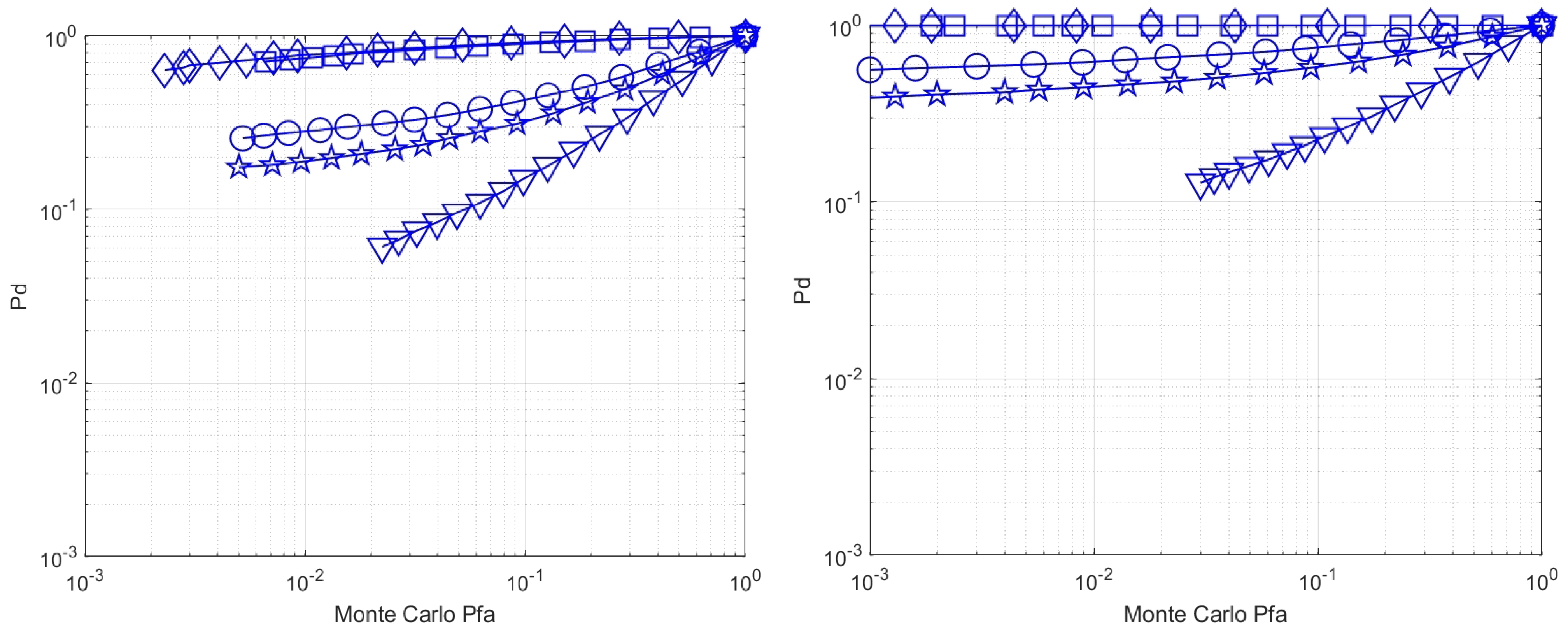
3.6. Receiver Operating Characteristic (ROC): Monte Carlo $P_{\mathrm{d}}$ versus Monte Carlo $P_{\mathrm{fa}}$

In this experiment, the receiver operating characteristic (Monte Carlo $P_{\mathrm{d}}$ versus Monte Carlo $P_{\mathrm{fa}}$, in short MC-$P_{\mathrm{d}}$ vs. MC-$P_{\mathrm{fa}}$) is computed for quadratic-form detectors. The results are reported in Figure 3.

For SC detectors and for the energy detector, the nominal $P_{\mathrm{fa}}$ is practically coincident with the Monte Carlo $P_{\mathrm{fa}}$, since the threshold is obtained using Monte Carlo simulation under ${\mathrm{H}}_0$. Therefore, the results were practically coincident with those of Section 3.5 and are not reported here. In contrast, for QF detectors, the nominal $P_{\mathrm{fa}}$ is practically coincident with the Monte Carlo $P_{\mathrm{fa}}$ only if the assumed distribution for the decision statistic ${\mathcal{T}}_0$ under ${\mathrm{H}}_0$ is correctly predicted.

By comparing the curves in Figure 3 with the corresponding ones in Figure 2, it follows that, when the data-record length increases from $T=2^{15}$ to $T=2^{19}$, the ROCs MC-$P_{\mathrm{d}}$ vs. MC-$P_{\mathrm{fa}}$ are practically coincident with the ROCs MC-$P_{\mathrm{d}}$ vs. nominal-$P_{\mathrm{fa}}$ for the QF detectors based on estimates of second- and 4th-order cyclic statistics or based on estimates of the cyclic CDF (Fourier coefficient of the indicator). In contrast, the ROC MC-$P_{\mathrm{d}}$ vs. MC-$P_{\mathrm{fa}}$ for the QF detectors based on estimates of the cyclic CDF (kernel-based estimator) presents irregularly spaced points and based on estimates of the cyclic pdf (kernel-based estimator) does not fit the corresponding ROC MC-$P_{\mathrm{d}}$ vs. nominal-$P_{\mathrm{fa}}$. Such a behavior for the ROCs of the detectors based on the cyclic CDF and pdf kernel estimators suggests that for these estimators the normalized estimation error is not Gaussian and, consequently, the threshold determined by (78) is not correct.

3.7. Monte Carlo $P_{\mathrm{fa}}$ versus Nominal or Design $P_{\mathrm{fa}}$

For detectors whose threshold is determined using Monte Carlo simulations (Section 3.2) we have, as expected, that the Monte Carlo (effective) $P_{\mathrm{fa}}$ is practically equal to the nominal or design $P_{\mathrm{fa}}$.

For detectors whose threshold is derived analytically, it make sense to check how far the effective Monte Carlo $P_{\mathrm{fa}}$ is from the nominal or design $P_{\mathrm{fa}}$.

In this experiment, the Monte Carlo $P_{\mathrm{fa}}$ versus the nominal $P_{\mathrm{fa}}$ is computed for the QF detectors. The results are reported in Figure 4.

According to the results of Section 3.6, when the data-record length increases from $T=2^{15}$ to $T=2^{19}$, the MC-$P_{\mathrm{fa}}$ approaches the nominal-$P_{\mathrm{fa}}$ for the QF detectors based on estimates of second- and 4th-order cyclic statistics or based on estimates of the cyclic CDF (Fourier coefficient of the indicator). Moreover, for the QF detectors based on estimates of the cyclic CDF (kernel-based estimator) and the cyclic pdf (kernel-based estimator), the effective Monte Carlo $P_{\mathrm{fa}}$ is far from the nominal or design $P_{\mathrm{fa}}$. Therefore, according to the results of Section 3.6, this fact could suggest that, for these detectors, the normalized estimation errors are not asymptotically complex normal. At least if the smoothing parameter b is chosen according to Silverman’s rule (30).

4. Discussion

The problem of cyclostationary signal detection is addressed in the fraction-of-time probability approach. In this approach, signals are modeled as single functions of time, rather than realizations of a stochastic process. Two classes of detectors are considered: the single-cycle detectors, and the quadratic-form detectors. The single-cycle detectors have a decision statistic that only depends on the received signal. Such a decision statistic is compared with a threshold that is derived from the available side data in the null hypothesis. In contrast, quadratic-form detectors have a decision statistic that depends on the received signal and side data in the null hypothesis and the threshold that can be derived analytically, provided that the decision statistic has a chi-squared fraction-of-time distribution under the null hypothesis. However, at the price of a modest performance degradation, the decision statistic can be computed using the received signal only, with no need of side data. For quadratic-form detectors, the covariance matrix is estimated with a subsampling procedure that is naturally derived in the fraction-of-time approach. For both single-cycle and quadratic-form detectors, a new class of cyclic statistical function measurements are considered: the cyclic cumulative distribution function, and the cyclic probability density function. The simulation results showed that these measurements can allow one to gain in performance with respect to measurements of cyclic autocorrelation, cyclic spectrum, and cyclic 4th-order moment. The advantage is particularly evident when the almost-periodically time-variant cumulative distribution and probability density functions exhibit harmonics whose strength is comparable with that of the continuous component. The effectiveness of the proposed detectors was tested on a FSK signal-of-interest in a severe noise and interference environment. Specifically, both additive stationary noise and narrow-band interference were present, with a power spectral density that completely overlapped that of the signal-of-interest. The SNR and SIR were both −20 dB. By operating at a cycle frequency equal to the symbol rate, a performance analysis was carried out using Monte Carlo simulations for the new proposed single-cycle and quadratic-form detectors based on measurements of the cylic CDF and pdf. Specifically, the probability of missed detection versus the data-record length and the receiver operating characteristics were estimated. Moreover, the performances were compared with those of analogous detectors based on measurements of cyclic autocorrelation, cyclic spectrum, and cyclic 4th-order moment measurements. The simulation results showed the better performance of the new proposed detectors. A further analysis was carried out to check the assumption made on the quadratic-form distribution that was exploited to analytically derive the detector threshold. Specifically, for all considered quadratic-form detectors, the nominal or design probability of false alarm (adopted to derive the threshold) was compared with the effective probability of false alarm obtained using Monte Carlo simulations. By increasing the data-record length, the values of the two probabilities of false alarm tended to be equal, except for the case of quadratic forms of measurements of cyclic CDF and pdf obtained using kernel-based estimators. Such a mismatch suggests that, unlike the case of zero cycle frequency, the normalized estimation error for kernel-based estimators is not asymptotically complex normal. Therefore, although the derived threshold provides satisfactory performance, this is not the best choice and better performances are expected to be obtained by properly modeling the distribution of the normalized estimation error and, hence, that of the quadratic-form detection statistic. Finally, note that the performance advantage of one detector over another strongly depends on the kind of signal-of-interest and its cyclic statistical functions. For example, for a pulse-amplitude-modulated signal with 50% duty-cycle rectangular pulse, detectors based on the cyclic autocorrelation and the 4th-order cyclic moment measurements outperformed those based on the cyclic CDF and pdf measurements.

References

1. Gardner, W.A. Statistical Spectral Analysis: A Nonprobabilistic Theory; Prentice-Hall: Englewood Cliffs, NJ, USA, 1987. [Google Scholar]
2. Napolitano, A. Cyclostationary Processes and Time Series: Theory, Applications, and Generalizations; Elsevier: Amsterdam, The Netherlands, 2019. [Google Scholar] [CrossRef]
3. Besicovitch, A.S. Almost Periodic Functions; Cambridge University Press: London, UK, 1932. [Google Scholar]
4. Gardner, W.A. Signal interception: A unifying theoretical framework for feature detection. IEEE Trans. Commun. 1988, COM-36, 897–906. [Google Scholar] [CrossRef]
5. Gardner, W.A.; Spooner, C.M. Signal interception: Performance advantages of cyclic feature detectors. IEEE Trans. Commun. 1992, 40, 149–159. [Google Scholar] [CrossRef]
6. Gardner, W.A.; Spooner, C.M. Detection and source location of weak cyclostationary signals: Simplifications of the maximum-likelihood receiver. IEEE Trans. Commun. 1993, 41, 905–916. [Google Scholar] [CrossRef]
7. Spooner, C.M.; Gardner, W.A. The cumulant theory of cyclostationary time-series. Part II: Development and applications. IEEE Trans. Signal Process. 1994, 42, 3409–3429. [Google Scholar] [CrossRef]
8. Dandawaté, A.V.; Giannakis, G.B. Statistical tests for presence of cyclostationarity. IEEE Trans. Signal Process. 1994, 42, 2355–2369. [Google Scholar] [CrossRef]
9. Napolitano, A. On cyclostationarity-based signal detection. In Proceedings of the XXVI European Signal Processing Conference (EUSIPCO 2018), Rome, Italy, 3–7 September 2018. [Google Scholar] [CrossRef]
10. Hurd, H.L.; Gerr, N.L. Graphical methods for determining the presence of periodic correlation. J. Time Ser. Anal. 1991, 12, 337–350. [Google Scholar] [CrossRef]
11. Enserink, S.; Cochran, D. On detection of cyclostationary signals. In Proceedings of the 1995 International Conference on Acoustics, Speech, and Signal Processing, Washington, DC, USA, 9–12 May 1995; Volume 3, pp. 2004–2007. [Google Scholar] [CrossRef]
12. Sirianunpiboon, S.; Howard, S.D.; Cochran, D. Detection of cyclostationarity using generalized coherence. In Proceedings of the IEEE International Conference on Acoustics, Speech and Signal Processing (ICASSP 2018), Calgary, AB, Canada, 15–20 April 2018. [Google Scholar]
13. Dehay, D.; Dudek, A.; Leskow, J. Subsampling for continuous-time almost periodically correlated processes. J. Stat. Plan. Inference 2014, 150, 142–158. [Google Scholar] [CrossRef]
14. Kim, K.; Akbar, I.; Bae, K.; Um, J.S.; Spooner, C.; Reed, J. Cyclostationary Approaches to Signal Detection and Classification in Cognitive Radio. In Proceedings of the 2nd IEEE International Symposium on New Frontiers in Dynamic Spectrum Access Networks (DySPAN 2007), Washington, DC, USA, 17–20 April 2007; pp. 212–215. [Google Scholar] [CrossRef]
15. Sutton, P.; Nolan, K.; Doyle, L. Cyclostationary Signatures in Practical Cognitive Radio Applications. IEEE J. Sel. Areas Commun. 2008, 26, 13–24. [Google Scholar] [CrossRef]
16. Haykin, S.; Thomson, D.J.; Reed, J.H. Spectrum Sensing for Cognitive Radio. Proc. IEEE 2009, 97, 849–877. [Google Scholar] [CrossRef]
17. Lundén, J.; Koivunen, V.; Huttunen, A.; Poor, H.V. Collaborative Cyclostationary Spectrum Sensing for Cognitive Radio Systems. IEEE Trans. Signal Process. 2009, 57, 4182–4195. [Google Scholar] [CrossRef]
18. Cohen, D.; Eldar, Y.C. Sub-Nyquist Cyclostationary Detection for Cognitive Radio. IEEE Trans. Signal Process. 2017, 65, 3004–3019. [Google Scholar] [CrossRef]
19. Yavorskyj, I.N.; Yuzefovych, R.; Kravets, I.B.; Matsko, I.Y. Properties of characteristics estimators of periodically correlated random processes in preliminary determination of the period of correlation. Radioelectron. Commun. Syst. 2012, 55, 335–348. [Google Scholar] [CrossRef]
20. Javorskyj, I.; Dehay, D.; Kravets, I. Component statistical analysis of second order hidden periodicities. Digit. Signal Process. 2014, 26, 50–70. [Google Scholar] [CrossRef]
21. Gardner, W.A. Statistically inferred time warping: Extending the cyclostationarity paradigm from regular to irregular statistical cyclicity in scientific data. EURASIP J. Adv. Signal Process. 2018, 2018, 59. [Google Scholar] [CrossRef]
22. Napolitano, A. Time-Warped Almost-Cyclostationary Signals: Characterization and Statistical Function Measurements. IEEE Trans. Signal Process. 2017, 65, 5526–5541. [Google Scholar] [CrossRef]
23. Das, S.; Genton, M.G. Cyclostationary Processes With Evolving Periods and Amplitudes. IEEE Trans. Signal Process. 2021, 69, 1579–1590. [Google Scholar] [CrossRef]
24. Sun, R.B.; Du, F.P.; Yang, Z.B.; Chen, X.F.; Gryllias, K. Cyclostationary Analysis of Irregular Statistical Cyclicity and Extraction of Rotating Speed for Bearing Diagnostics With Speed Fluctuations. IEEE Trans. Instrum. Meas. 2021, 70, 3514011. [Google Scholar] [CrossRef]
25. Leśkow, J.; Napolitano, A. Foundations of the functional approach for signal analysis. Signal Process. 2006, 86, 3796–3825. [Google Scholar] [CrossRef]
26. Gardner, W.A. Cyclostationarity.com. 2018. Available online: https://cyclostationarity.com (accessed on 1 October 2023).
27. Napolitano, A.; Gardner, W.A. Fraction-of-time probability: Advancing beyond the need for stationarity and ergodicity assumptions. IEEE Access 2022, 10, 34591–34612. [Google Scholar] [CrossRef]
28. Gardner, W.A. Transitioning away from stochastic process models. J. Sound Vib. 2023, 565, 117871. [Google Scholar] [CrossRef]
29. Kac, M.; Steinhaus, H. Sur les fonctions indépendantes (IV) (Intervalle infini). Stud. Math. 1938, 7, 1–15. [Google Scholar] [CrossRef]
30. Kac, M. Statistical Independence in Probability, Analysis and Number Theory; The Mathematical Association of America: Washington, DC, USA, 1959. [Google Scholar]
31. Gardner, W.A.; Brown, W.A. Fraction-of-time probability for time-series that exhibit cyclostationarity. Signal Process. 1991, 23, 273–292. [Google Scholar] [CrossRef]
32. Gardner, W.A.; Spooner, C.M. The cumulant theory of cyclostationary time-series. Part I: Foundation. IEEE Trans. Signal Process. 1994, 42, 3387–3408. [Google Scholar] [CrossRef]
33. Izzo, L.; Napolitano, A. The higher-order theory of generalized almost-cyclostationary time-series. IEEE Trans. Signal Process. 1998, 46, 2975–2989. [Google Scholar] [CrossRef]
34. Miao, H.; Zhang, F.; Tao, R. A general fraction-of-time probability framework for chirp cyclostationary signals. Signal Process. 2021, 179, 107820. [Google Scholar] [CrossRef]
35. Zemanian, A.H. Distribution Theory and Transform Analysis; Dover: New York, NY, USA, 1987. [Google Scholar]
36. Dehay, D.; Leśkow, J.; Napolitano, A. Time average estimation in the fraction-of-time probability framework. Signal Process. 2018, 153, 275–290. [Google Scholar] [CrossRef]
37. Parzen, E. On Estimation of a Probability Density Function and Mode. Ann. Math. Stat. 1962, 33, 1065–1076. [Google Scholar] [CrossRef]
38. Rosenblatt, M. Curve Estimates. Ann. Math. Stat. 1971, 42, 1815–1842. [Google Scholar] [CrossRef]
39. Serfling, R.J. Approximation Theorems of Mathematical Statistics; John Wiley & Sons, Inc.: Hoboken, NJ, USA, 1980. [Google Scholar]
40. Castellana, J.; Leadbetter, M. On smoothed probability density estimation for stationary processes. Stoch. Process. Their Appl. 1986, 21, 179–193. [Google Scholar] [CrossRef]
41. Shevgunov, T.; Napolitano, A. Fraction-of-time density estimation based on linear interpolation of time series. In Proceedings of the 2021 Systems of Signals Generating and Processing in the Field of on Board Communications, Moscow, Russia, 16–18 March 2021. [Google Scholar] [CrossRef]
42. Dehay, D. Spectral analysis of the covariance of the almost periodically correlated processes. Stoch. Process. Their Appl. 1994, 50, 315–330. [Google Scholar] [CrossRef]
43. Dehay, D.; Leśkow, J. Functional limit theory for the spectral covariance estimator. J. Appl. Probab. 1996, 33, 1077–1092. [Google Scholar] [CrossRef]
44. Leskow, J. Asymptotic normality of the spectral density estimators for almost periodically correlated stochastic processes. Stochatic Process. Their Appl. 1994, 52, 351–360. [Google Scholar] [CrossRef]
45. Napolitano, A. Generalizations of Cyclostationary Signal Processing: Spectral Analysis and Applications; John Wiley & Sons Ltd.: Hoboken, NJ, USA; IEEE Press: Piscataway, NJ, USA, 2012. [Google Scholar] [CrossRef]
46. Shevgunov, T.; Efimov, E.; Guschina, O. Estimation of a Spectral Correlation Function Using a Time-Smoothing Cyclic Periodogram and FFT Interpolation–2N-FFT Algorithm. Sensors 2023, 23, 215. [Google Scholar] [CrossRef] [PubMed]
47. Dandawaté, A.V.; Giannakis, G.B. Nonparametric polyspectral estimators for kth-order (almost) cyclostationary processes. IEEE Trans. Inf. Theory 1994, 40, 67–84. [Google Scholar] [CrossRef]
48. Dandawaté, A.V.; Giannakis, G.B. Asymptotic theory of mixed time averages and kth-order cyclic-moment and cumulant statistics. IEEE Trans. Inf. Theory 1995, 41, 216–232. [Google Scholar] [CrossRef]
49. Spooner, C.M. Cyclostationary Signal Processing: Understanding and Using the Statistics of Communication Signals. 2015. Available online: https://cyclostationary.blog (accessed on 1 October 2023).
50. Picinbono, B. Second-order complex random vectors and normal distributions. IEEE Trans. Signal Process. 1996, 44, 2637–2640. [Google Scholar] [CrossRef]
51. Van Trees, H.L. Detection, Estimation, and Modulation Theory. Part I; John Wiley & Sons, Inc.: New York, NY, USA, 1971. [Google Scholar]
52. Huang, G.; Tugnait, J.K. On Cyclostationarity Based Spectrum Sensing Under Uncertain Gaussian Noise. IEEE Trans. Signal Process. 2013, 61, 2042–2054. [Google Scholar] [CrossRef]
Figure 1. Monte Carlo P md versus T. Energy detector (black): (∗). Quadratic form detectors (blue) and single-cycle detectors (green): (▽) cyclic pdf (kernel-based estimator); (□) cyclic CDF (Fourier coefficient of the indicator); (◯) cyclic autocorrelation (cyclic correlogram); (◊) cyclic CDF (kernel-based estimator); (✶) cyclic 4th-order moment.
Inventions 08 00152 g001
Figure 2. ROC: Monte Carlo P d versus nominal P fa . (Left) T = 2 15 T s ; (Right) T = 2 19 T s . Energy detector (black): (*). Quadratic form detectors (blue) and single cycle detectors (green): (▽) cyclic pdf (kernel-based estimator); (□) cyclic CDF (Fourier coefficient of the indicator); (◯) cyclic autocorrelation (cyclic correlogram); (◊) cyclic CDF (kernel-based estimator); (✶) cyclic 4th-order moment.
Inventions 08 00152 g002
Figure 3. ROC: Monte Carlo P d versus Monte Carlo P fa . (Left) T = 2 15 T s ; (Right) T = 2 19 T s . Quadratic form detectors (blue): (▽) cyclic pdf (kernel-based estimator); (□) cyclic CDF (Fourier coefficient of the indicator); (◯) cyclic autocorrelation (cyclic correlogram); (◊) cyclic CDF (kernel-based estimator); (✶) cyclic 4th-order moment.
Inventions 08 00152 g003
Figure 4. Monte Carlo (effective) P fa is versus nominal or design P fa . (Left) T = 2 15 T s ; (Right) T = 2 19 T s . Quadratic form detectors (blue): (▽) cyclic pdf (kernel-based estimator); (□) cyclic CDF (Fourier coefficient of the indicator); (◯) cyclic autocorrelation (cyclic correlogram); (◊) cyclic CDF (kernel-based estimator); (✶) cyclic 4th-order moment. Black line: Monte Carlo P fa = nominal P fa .
Inventions 08 00152 g004
Disclaimer/Publisher’s Note: The statements, opinions and data contained in all publications are solely those of the individual author(s) and contributor(s) and not of MDPI and/or the editor(s). MDPI and/or the editor(s) disclaim responsibility for any injury to people or property resulting from any ideas, methods, instructions or products referred to in the content.