The Current Spectrum Formation of a Non-Periodic Signal: A Differential Approach

Abstract

The paper deals with the problem of forming spectra of non-periodic signals in real-time. The disadvantage of the existing approaches is the dependence of the formed spectrum on time as a parameter and the possibility of obtaining the signal spectrum in its original definition only for a fixed time, as well as a high amount of computation. In this regard, a computationally efficient algorithm is proposed for forming a spectrum of non-periodic functions on a time interval that is constantly updated with a given sampling step, which ensures the invariance of the generated spectrum to time as a parameter. The algorithm is based on obtaining differential equations that are based on generalized differentiation with respect to a variable time interval of spectral components and their solving while using the fourth-order Runge–Kutta method. A numerical simulation of the developed algorithm was performed using the MATLAB mathematical modeling package using the example of a substantially non-linear function. Based on the practical results, a comparative evaluation of computational and time complexity has been performed in solving the problem. Based on the obtained experimental results, it is concluded that it is possible to effectively use the proposed algorithm to calculate the current spectrum of non-periodic functions with the requirement of small sampling steps, i.e., when calculating the spectrum in real-time.

1. Introduction

The analysis of the spectra of current physical processes in real time is one of the most important tasks of signal processing [1,2,3]. This problem is relevant, not only in the analysis of various control and communication systems, but it also finds wide application in navigation systems, seismology, astronomy, and others.

Presently, this problem is solved either by calculating the Fourier transform for function f(t) with a variable upper limit of integration [4,5,6], or the classical Fourier-series expansion [7,8,9] on a time interval T_i (T_i = T_i+1 + ΔT; i = 1, 2, …) constantly updated with a given sampling interval ΔT:

$$\begin{gathered} f\left(t\right)=\frac{a_0}{2}+{\displaystyle \sum }_{k=1}^{\infty }{a}_{k}cosk\frac{2\pi }{T_i}t+b_{k}sink\frac{2\pi }{T_i}t, \\ {a}_k=\frac{2}{T_i}{\int }_0^{T_i}f\left(t\right)cosk\frac{2\pi }{T_i}dt, \\ {b}_k=\frac{2}{T_i}{\int }_0^{T_i}f\left(t\right)sink\frac{2\pi }{T_i}dt,k=0,1,2,\dots . \end{gathered}$$

(1)

In the first case, the spectrum that formed depends on time as a parameter, thus obtaining the signal spectrum in its classical definition (that is, independent of time) is possible only at a fixed t. In the second case, there is a large amount of computational costs [9] to reduce which methods of discrete transformation, such as Fast Fourier Transform (FFT) [2,10,11], are widely used. The amount of FFT calculations that require ~Nlog₂N multiplication operations [10,12] is somewhat reduced as compared to traditional conversion. This does not radically change the situation, since, when calculating the current spectrum, this number of multiplication operations must be performed at each new time step with a constantly increasing time interval. Such shortcomings of both approaches create significant difficulties in their practical use.

2. Theoretical Assumptions

2.1. Task Definition

In this regard, there is a need to develop such an algorithm for calculating the spectrum of non-periodic functions on a time interval that was updated with a given sampling interval, which, on one hand, does not require large computational costs and, on the other hand, provides the formation of the spectrum in its original–classical, definition (1).

2.2. Task Solution

For the construction of this algorithm, the variations $\Delta a_k$ and $\Delta b_k$ of spectral coefficients a_k and b_k that are caused by a change in the time interval T_i by the value ΔT are preliminarily found. Using the equation of generalized differentiation by variable T_i (Leibniz formula), we have for the corresponding spectral components:

$$\begin{gathered} \begin{array}{cc}\hfill \frac{\partial a_k}{\partial T_i}& =-\frac{2}{T_i^2}{\int }_0^{T_i}f\left(t\right)\mathit{cos}k\frac{2\pi }{T_i}tdt\hfill \\ & +\frac{2}{T_i}\left(\frac{2\pi k}{T_i^2}{\int }_0^{T_i}f\left(t\right)t\mathit{sin}k\frac{2\pi }{T_i}tdt+f\left(T_i\right)\mathit{cos}k\frac{2\pi }{T_i}{T}_i\right),\hfill \end{array} \\ \begin{array}{cc}\hfill \frac{\partial b_k}{\partial T_i}& =-\frac{2}{T_i^2}{\int }_0^{T_i}f\left(t\right)\mathit{sin}k\frac{2\pi }{T_i}tdt\hfill \\ & +\frac{2}{T_i}\left(-\frac{2\pi k}{T_i^2}{\int }_0^{T_i}f\left(t\right)t\mathit{cos}k\frac{2\pi }{T_i}tdt+f\left(T_i\right)\mathit{sin}k\frac{2\pi }{T_i}{T}_i\right).\hfill \end{array} \end{gathered}$$

(2)

Considering further that

$$\begin{gathered} \frac{\partial a_k}{\partial k}=-\frac{2}{T_i}\frac{2\pi }{T_i}{\int }_0^{T_i}f\left(t\right)t\mathit{sin}k\frac{2\pi }{T_i}tdt, \\ \frac{\partial b_k}{\partial k}=\frac{2}{T_i}\frac{2\pi }{T_i}{\int }_0^{T_i}f\left(t\right)t\mathit{cos}k\frac{2\pi }{T_i}tdt, \end{gathered}$$

(3)

Equation (2) is written as

$$\begin{gathered} \frac{\partial a_k}{\partial T_i}=-\frac{1}{T_i}{a}_k-\frac{k}{T_i}\frac{\partial a_k}{\partial k}+\frac{2}{T_i}f\left(T_i\right), \\ \frac{\partial b_k}{\partial T_i}=-\frac{1}{T_i}{b}_k-\frac{k}{T_i}\frac{\partial b_k}{\partial k}. \end{gathered}$$

(4)

Since k changes discretely in increments of one, an approximation is possible $\frac{\partial a_k}{\partial k}=a_k-a_{k-1},$ $\frac{\partial b_k}{\partial k}=b_k-b_{k-1},$ which allows us to finally write the differential equations that describe the dynamics of changes in spectral coefficients, as follows:

$$\begin{gathered} \frac{\partial a_k}{\partial T_i}=-\frac{1}{T_i}\cdot \left[\left(1+k\right)a_k-k{a}_{k-1}\right]+\frac{2}{T_i}f\left(T_i\right), \\ \frac{\partial b_k}{\partial T_i}=-\frac{1}{T_i}\cdot \left[\left(1+k\right)b_k-k{b}_{k-1}\right]. \end{gathered}$$

(5)

The search for the solution of differential Equation (5) under known initial conditions leads to the formulation of the Cauchy problem, where the initial conditions are: $T_0=T_{i-1}$ is the end time of the previous time interval, $a_0=a_{i-1}$ and $b_0=b_{i-1}$ are the coefficients that are calculated on the previous interval according to the Equation (1).

In practice, the most common method for solving ordinary differential equations $\dot{y}=q\left(x,y\right)$ is the fourth-order Runge–Kutta method [13,14,15]. In this case, each step calculates the value of the function $q\left(x,y\right)$ of the right side four times; each value $y\left[i+1\right]$ is obtained based on the previous one, according to the equation:

$$y\left[i+1\right]=y\left[i\right]+\Delta y\left[i\right],$$

(6)

where

$$\begin{gathered} \Delta y\left[i\right]=h/6\left(K_1+2K_2+2K_3+K_4\right); \\ {K}_1=q\left(x\left[i\right],y\left[i\right]\right); \\ {K}_2=q\left(x\left[i\right]+h/2,y\left[i\right]+h{K}_1/2\right); \\ {K}_3=q\left(x\left[i\right]+h/2,y\left[i\right]+h{K}_2/2\right); \\ {K}_4=q\left(x\left[i\right]+h,y\left[i\right]+h{K}_3\right); \end{gathered}$$

h is the size of the grid step according to the argument x.

When calculation spectral coefficients a_k and b_k in Equation (5) in this scheme, the argument x[i] is the variable T_i, the argument y[i] is the coefficients a_k[i], b_k[i]. Consequently, the calculation procedure takes the form:

$$\begin{gathered} K_{a1}=-\frac{\left(1+k\right)a_k\left[i\right]-k{a}_{k-1}\left[i\right]}{T_i}+\frac{2}{T_i}f\left(T_i\right), \\ {K}_{a2}=-\frac{\left(1+k\right)(a_k\left[i\right]+h\frac{K_{1a}}{2})-k(a_{k-1}\left[i\right]+h\frac{K_{1a}}{2})}{T_i+\frac{h}{2}}+\frac{2}{T_i+h/2}f\left(T_i+h/2\right), \\ K_{a3}=-\frac{\left(1+k\right)(a_k\left[i\right]+h\frac{K_{2a}}{2})-k(a_{k-1}\left[i\right]+h\frac{K_{2a}}{2})}{T_i+h/2}+\frac{2}{T_i+h/2}f\left(T_i+h/2\right), \\ K_{a4}=-\frac{\left(1+k\right)\left(a_k\left[i\right]+h{K}_{3a}\right)-k\left(a_{k-1}\left[i\right]+h{K}_{3a}\right)}{T_i+h}+\frac{2}{T_i+h}f\left(T_i+h\right), \\ \Delta a_k\left[i\right]=h/6\left(K_{a1}+2K_{a2}+2K_{a3}+K_{a4}\right), \\ {a}_k\left[i+1\right]=a_k\left[i\right]+\Delta a_k\left[i\right]; \\ {K}_{b1}=-\frac{\left(1+k\right)b_k\left[i\right]-k{b}_{k-1}\left[i\right]}{T_i}, \\ {K}_{b2}=-\frac{\left(1+k\right)(b_k\left[i\right]+h\frac{K_{1b}}{2})-k(b_{k-1}\left[i\right]+h\frac{K_{1b}}{2})}{T_i+h/2}, \\ {K}_{b3}=-\frac{\left(1+k\right)(b_k\left[i\right]+h\frac{K_{2b}}{2})-k(b_{k-1}\left[i\right]+h\frac{K_{2b}}{2})}{T_i+h/2}, \\ {K}_{b4}=-\frac{\left(1+k\right)\left(b_k\left[i\right]+h{K}_{3b}\right)-k\left(b_{k-1}\left[i\right]+h{K}_{3b}\right)}{T_i+h}, \\ \Delta b_k\left[i\right]=h/6\left(K_{b1}+2K_{b2}+2K_{b3}+K_{b4}\right), \\ {b}_k\left[i+1\right]=b_k\left[i\right]+\Delta b_k\left[i\right]. \end{gathered}$$

(7)

The accuracy of the solution of which is largely influenced by the value of the step h of the grid, a numerical estimate of the accuracy of determining the dynamics of changes in the spectral coefficients, given below, was made to analyse the computational efficiency of the obtained equations.

3. Results

3.1. Experimental Design

The numerical simulation of the developed algorithm was carried out using the MATLAB (The MathWorks, Inc., USA) mathematical modeling package, which allows for additionally estimating the time costs for the solution. To assess the accuracy of the proposed algorithms, three essentially nonlinear functions were considered as a test function:

$$\begin{gathered} f\left(t\right)=\frac{\mathit{sin}(t)}{1+2{\mathit{cos}}^{2}2t}\cdot e^{-0.015t}; \\ f_2\left(t\right)={\mathit{sin}}^{2}t+2e^{0.05t}; \\ {f}_3\left(t\right)=\left(0.5t+\mathit{cos}(t\right))\cdot e^{-0.2t}. \end{gathered}$$

(8)

The spectra of this function were constructed for time intervals T₀ = 50.1 s and T₀ = 51.0 s both using classical integral transformations (1) to form the reference spectra and while using the proposed algorithm for the sampling interval ΔT = 0.001 s. The grid step h for the Runge–Kutta algorithm was assumed to be equal h = 0.0001.

The evaluation of the comparative results of modeling the values of spectral coefficients a_k[i] and b_k[i] obtained using the integral transformation (1) and the proposed algorithm was carried out according to the following criteria:

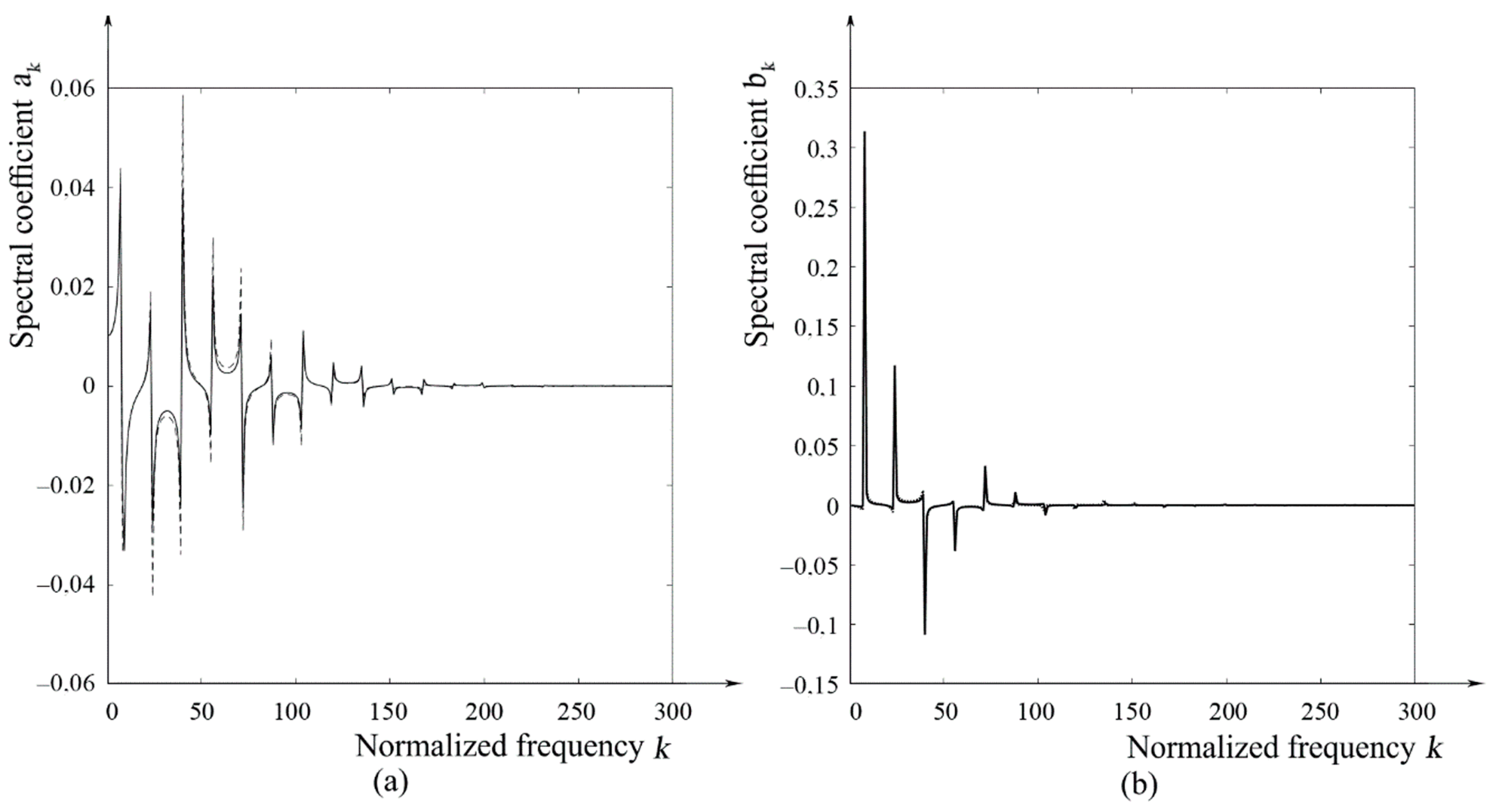
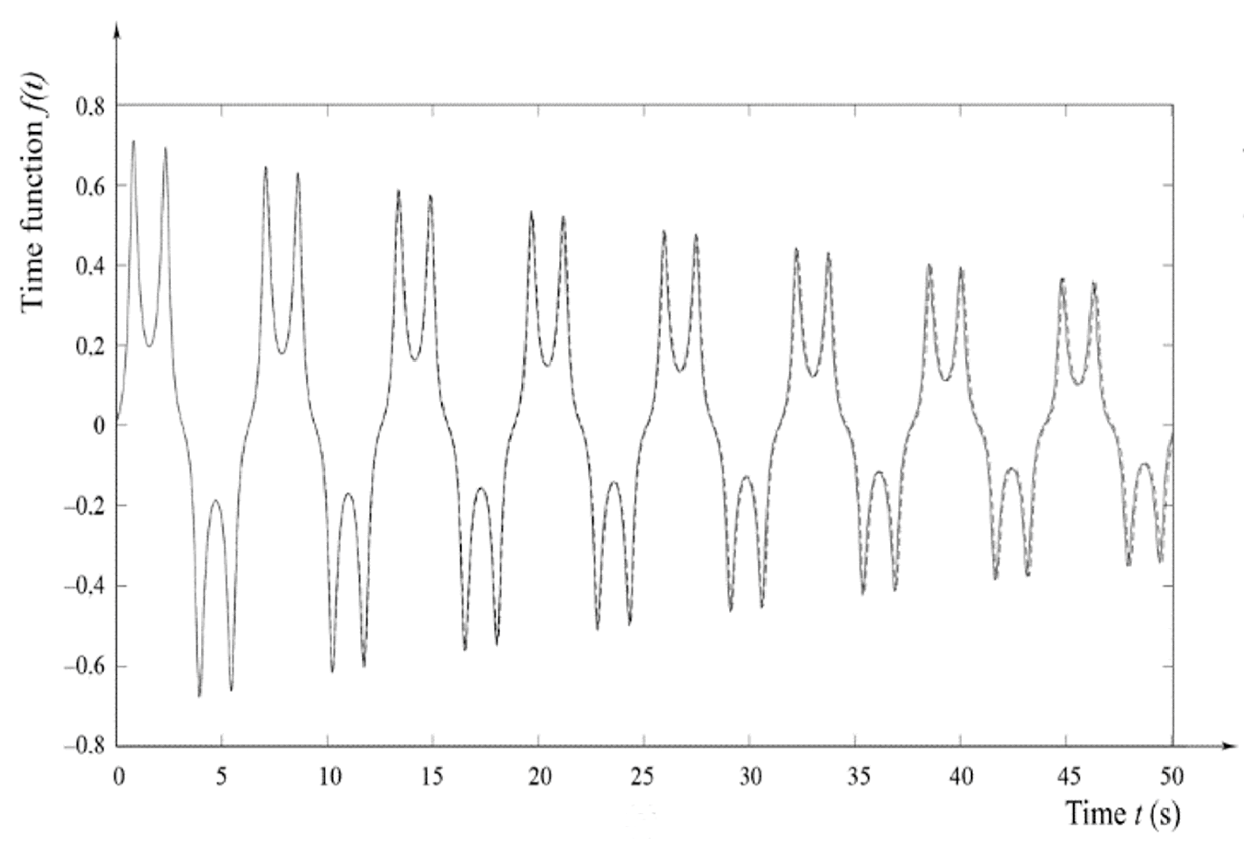
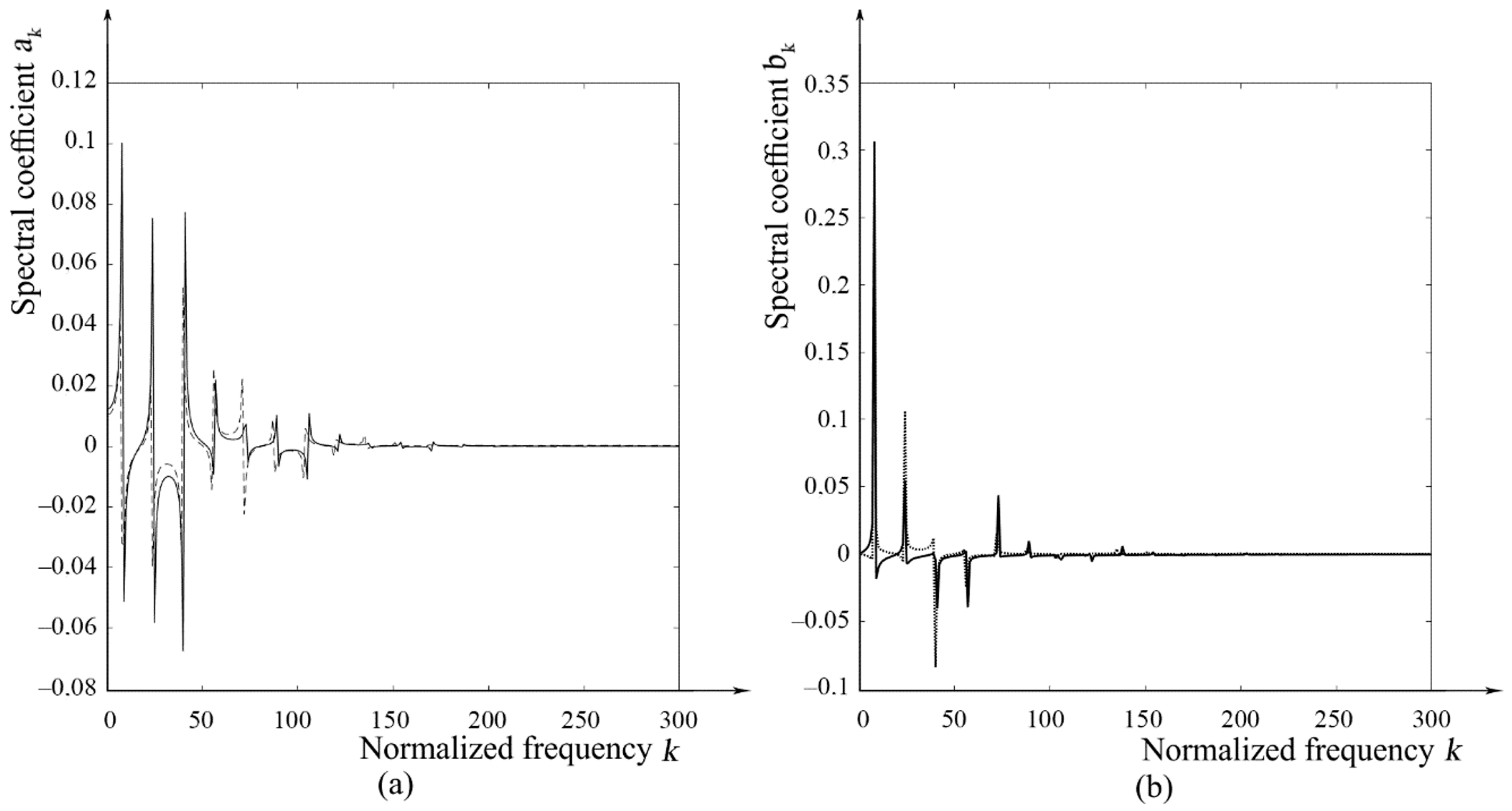
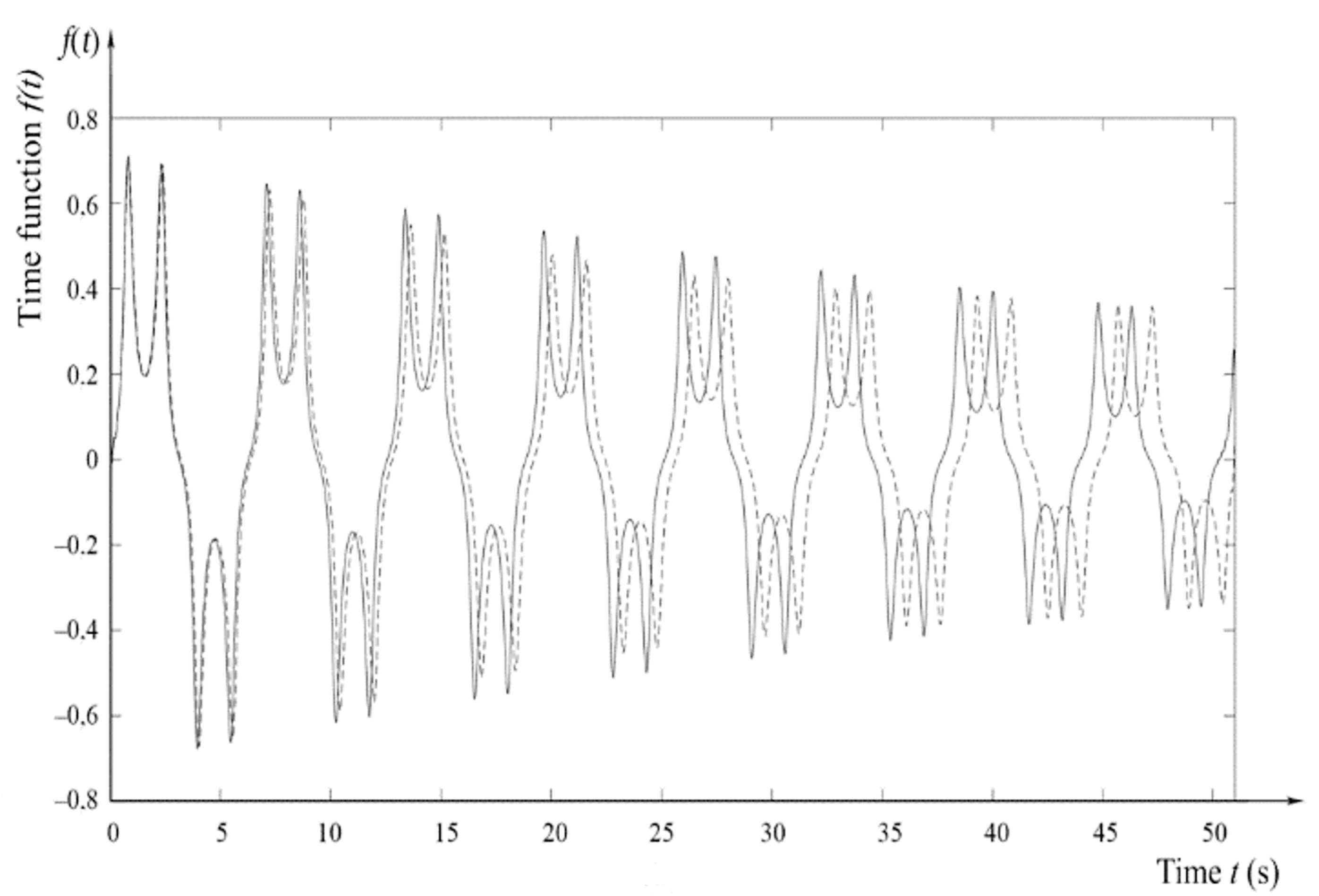
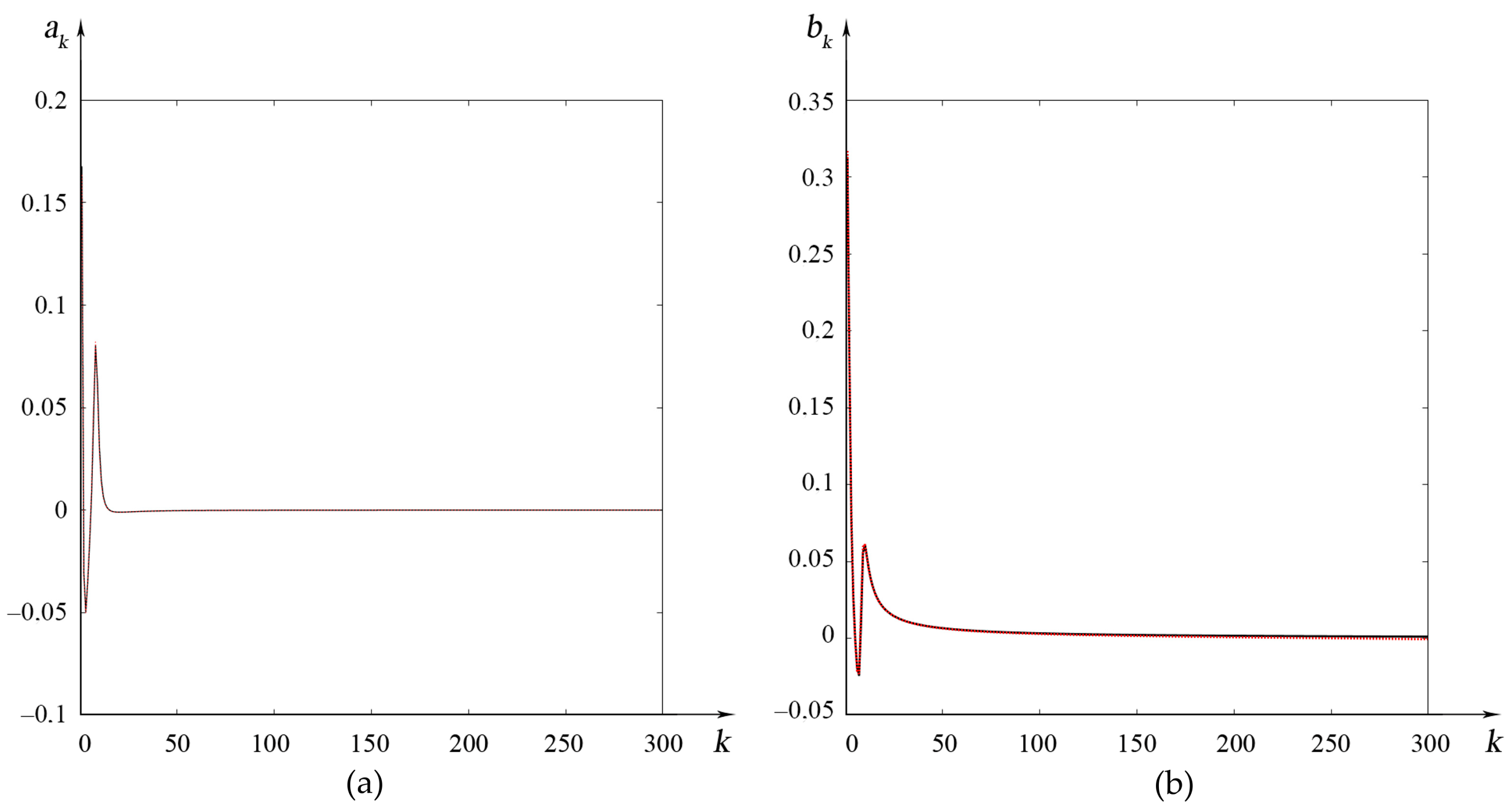
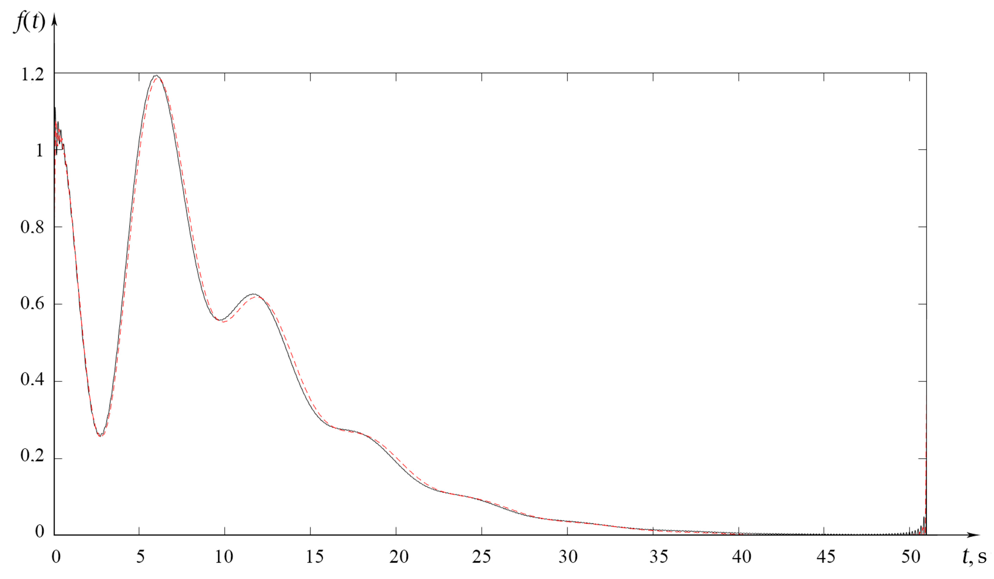
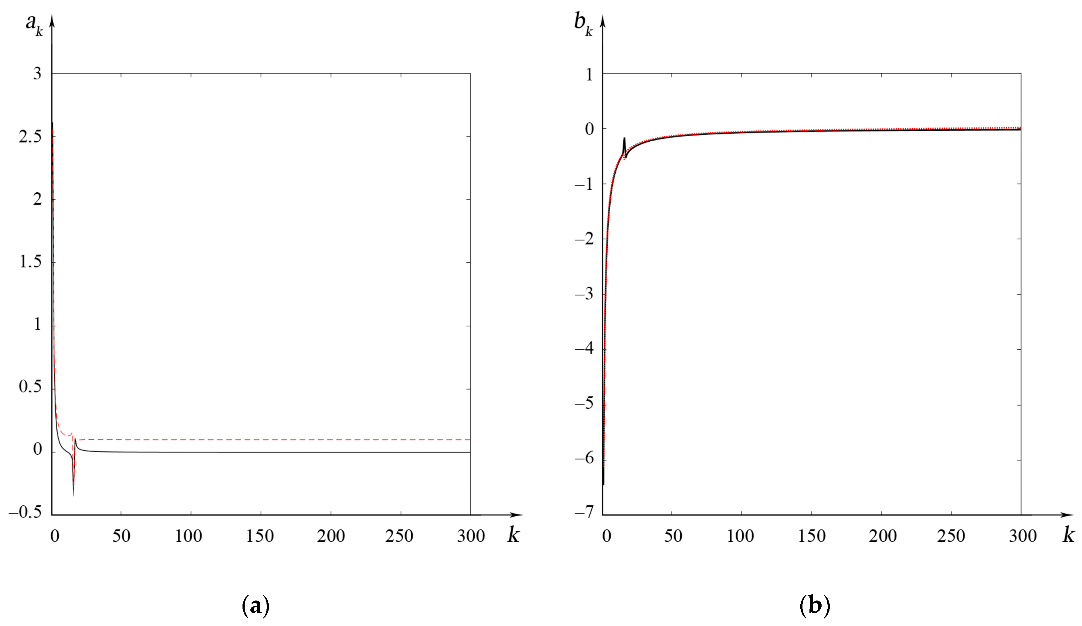
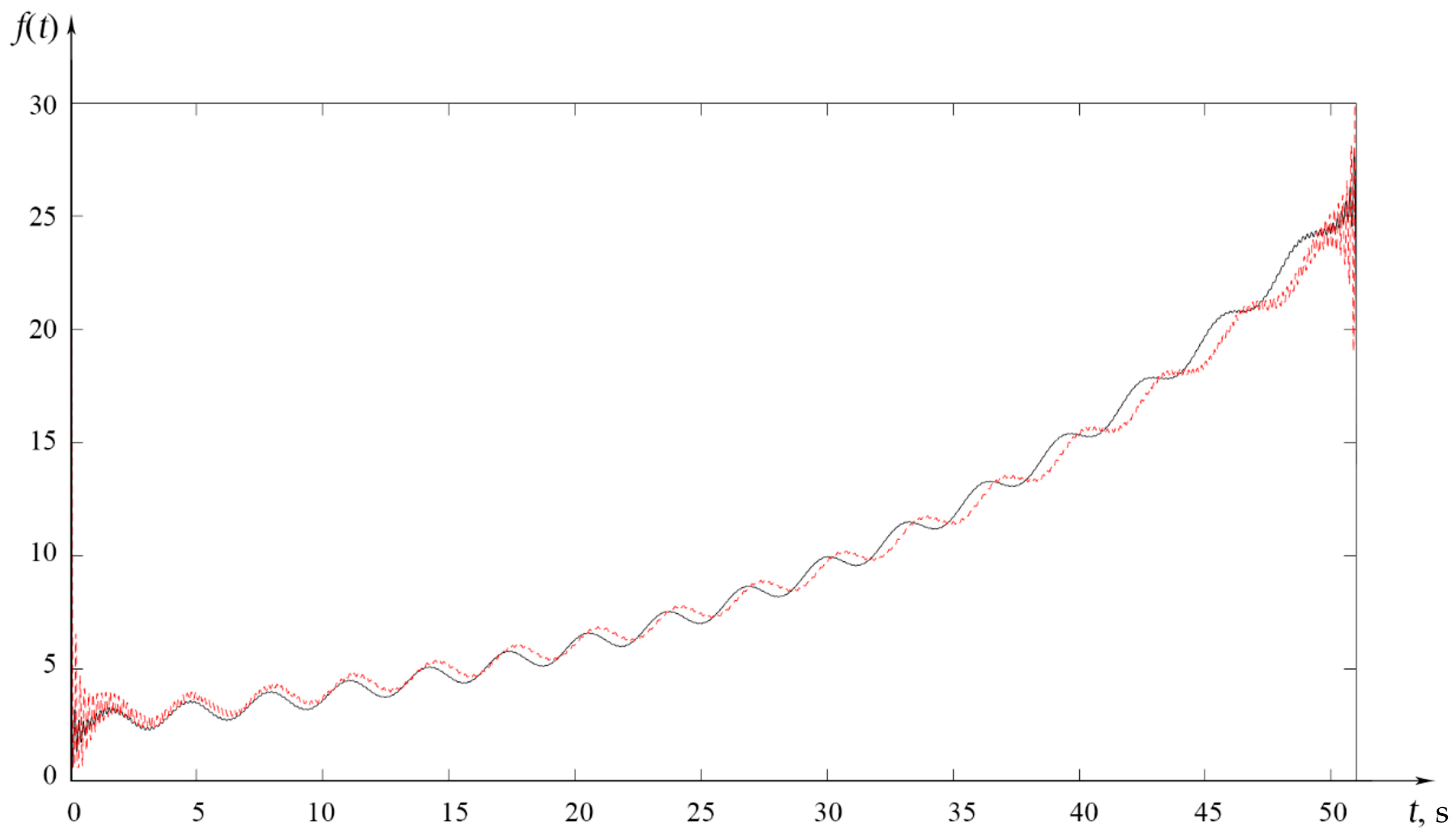
• By graphical representation of calculated coefficients and reconstructed signals;
• On the Central Processing Unit (CPU) time during calculations;
• Relative performance, defined as the percentage of the difference between the time estimates of calculations performed using the classical (see Equation 1) and the developed algorithms, and the time of calculation using the classical algorithm; and,
• Based of the standard deviations analysis of the spectral coefficients values a_k[i] and b_k[i] calculated by the above algorithm from the reference values a_kr[i] and b_kr[i] calculated by the integral transformation (1).

The estimation of the CPU operation time during the calculations was made on the personal computer Intel Core i5-2500 3.30 GHz.

3.2. Numerical Modelling

Figure 1 shows the graphical results of modeling the spectral coefficients a_kr[i] and b_kr[i] (solid line), a_k[i] and b_k[i] (dotted line) that were obtained using the traditional and the proposed algorithms for the function f₁(t) in the time interval T₀ = 50.1 s, respectively.

The CPU operating time in the calculation using the integral transformation (1) was 1.7188 s, in the calculation according to the proposed algorithm −0.0625 s. The relative performance of the proposed algorithm in this case amounted to 96.4%. The mean square deviations of the spectral coefficients were: for the coefficients a_k[i] s₁ = 0.0020; and, for the coefficients b_k[i] s₂ = 0.0018.

The time signals for the f₁(t) function that was reconstructed from the received spectra are shown in Figure 2. Here, a solid line shows the restored signal for 50.1 s, as calculated from the spectrum that was obtained using the integral transformation (1), and dotted line from the spectrum obtained using the proposed algorithm.

At this time interval (for 10² time samples of the current spectrum formation), the coincidence of the spectral coefficients a_k[i] and b_k[i] calculated by the proposed algorithm with the reference values a_kr[i] and b_kr[i] calculated by the integral transformation (1), as well as the restored signals, is almost complete, as can be seen from the simulation results. At the same time, the time spent on the process of calculating the current spectrum in the proposed algorithm decreased by more than 96% when compared to the classical one.

Figure 3 shows the graphical results of modeling the spectral coefficients a_kr[i] and b_kr[i] (solid line), a_k[i] and b_k[i] (dotted line) that were obtained using the traditional and the proposed algorithms for the function f₁(t) in the time interval T₀ = 51.0 s, respectively.

The CPU operating time in the calculation using the integral transformation (1) was 1.8750 s, in the calculation according to the proposed algorithm −0.3594 s. The relative performance of the proposed algorithm in this case amounted to 80.8%. The mean square deviations of the spectral coefficients were: for the coefficients a_k[i] s₁ = 0.0147; and, for the coefficients b_k[i] s₂ = 0.0089.

The time signals for the f₁(t) function reconstructed from the obtained spectra are shown in Figure 4. Here, a solid line shows the recovered signal for 51.0 s, calculated from the spectrum obtained using the integral transformation (1), and dotted line from the spectrum that was obtained using the proposed algorithm.

At this time interval T₀ = 51.0 s (for 10³ time samples of the current spectrum formation), the coincidence of the spectral coefficients that were calculated by the given algorithm with the reference ones, as well as the reconstructed signals, has somewhat deteriorated when compared to the previous time interval, which is due to the accumulation of step-by-step calculation errors in the proposed recurrent algorithm. However, nevertheless, the time spent on the process of calculating the current spectrum in the proposed algorithm was still more than 80% less as compared to the classical one.

Since the proposed algorithm shows fairly stable results for small time intervals, the results of numerical simulation for the f₂(t) and f₃(t) functions are immediately presented for the time interval T₀ = 51.0 s, after which a generalized evaluation of the results for all three functions for the time intervals T₀ = 50.1 s and T₀ = 51.0 s.

Figure 5 shows the graphical results of modeling the spectral coefficients a_kr[i] and b_kr[i] (solid line), a_k[i] and b_k[i] (dotted line) that were obtained using the traditional and the proposed algorithms for the function f₂(t) in the time interval T₀ = 51.0 s, respectively.

The CPU operating time in the calculation using the integral transformation (1) was 1.5938 s, in the calculation according to the proposed algorithm −0.3281 s. The relative performance of the proposed algorithm in this case amounted to 79.4%. The mean square deviations of the spectral coefficients were: for the coefficients a_k[i] s₁ = 0.0006512; and, for the coefficients b_k[i] s₂ = 0.00082342.

Figure 6 shows the time signals for the f₂(t) function that was reconstructed from the obtained spectra. Here, a solid line shows the recovered signal for 51.0 s, which was calculated from the spectrum obtained using the integral transformation (1), and the dotted line from the spectrum that was obtained using the proposed algorithm.

Figure 7 shows the graphical results of modeling the spectral coefficients a_kr[i] and b_kr[i] (solid line), a_k[i] and b_k[i] (dotted line) obtained while using the traditional and the proposed algorithms for the function f₃(t) in the time interval T₀ = 51.0 s, respectively.

The CPU operating time in the calculation using the integral transformation (1) was 1.6250 s, in the calculation according to the proposed algorithm 0.3281 s. The relative performance of the proposed algorithm in this case amounted to 79.8%. The mean square deviations of the spectral coefficients were: for the coefficients a_k[i] s₁ = 0.0172; and, for the coefficients b_k[i] s₂ = 0.0342.

Figure 8 shows the time signals for the f₃(t) function that was reconstructed from the obtained spectra. Here, a solid line shows the recovered signal for 51.0 s, as calculated from the spectrum that was obtained using the integral transformation (1), and dotted line from the spectrum obtained using the proposed algorithm.

3.3. Evaluation of Numerical Modelling

Table 1. Generalized evaluation of the results of numerical modeling.

Time Interval	T0 = 50.1 s			T0 = 51.0 s
Evaluation Criterion	Standard Deviation for ak[i]	Standard Deviation for bk[i]	Performance, %	Standard Deviation for ak[i]	Standard Deviation for bk[i]	Performance, %
f1(t)	0.0020	0.0018	96.4	0.0147	0.0089	80.8
f2(t)	0.000066253	0.0004806	97.0	0.0006512	0.00082342	79.4
f3(t)	0.0020	0.0107	98.8	0.0172	0.0342	79.8

provides a generalized estimate of the results of numerical simulation for functions f₁(t), f₂(t), and f₃(t) at time intervals T₀ = 50.1 s and T₀ = 51.0 s.

As follows from the results, for all three functions, the performance estimates have approximately the same values—the relative performance of the process of calculating the current spectrum for the time interval T₀ = 50.1 s is more than 96%, for T₀ = 51.0 s about 80%.

In order to assess the effect of the value of the time interval on the growth of errors that were caused by the accumulation of incremental error calculation in the proposed algorithm, for the considered nonlinear functions are constructed based on changes (Figure 9) in the values of standard deviation values of the spectral coefficients a_k[i] (dashed line) and b_k[i] (solid line) recovered signals in the interval from 50.1 to 60.0 s.

From the analysis of these dependencies, we can conclude that the temporal nature of the mismatch of spectral coefficients depends on the type of function being modeled and the nature of its nonlinearity. Accordingly, for the function f₁(t) deviation of the recovered spectrum above the value of 0.005 is observed at 52 s, for the function f₂(t) at 59 s, for the function f₃(t) at 51 s. In this case, for 51 s (Figure 8), the recovered signal generally shows a slight deviation, but fluctuations that occur at the spectrum boundaries lead to an increase in the standard deviations of the spectral coefficients.

4. Conclusions

The results of numerical modeling allow for drawing a conclusion regarding the possibility of effective practical use of the proposed approach to the calculation of the current spectrum of non-periodic functions under the requirement of small sampling steps (i.e., when calculating the spectrum in real time). In comparison with the most effective method of spectral characteristics formation—FFT, the developed algorithms have the following advantages. Firstly, their number of multiplication and addition operations at each step is constant and it does not depend on the increasing number N of time samples of the signal, being determined by the step of its sampling and the current value T of the increasing time interval and, secondly, this number of operations is incommensurably small when compared to the constantly increasing number of FFT operations Nlog₂N at the current interval.

The implementation of the developed algorithm is particularly relevant in systems of measurement and the spectral processing of broadband signals in real time–telecommunications, navigation, and others.

References

1. Dyakonov, V. Modern digital spectrum analyzers. Components Technol. 2010, 5, 185–195. [Google Scholar]
2. Isermann, R.; Münchhof, M. Identification of Dynamic Systems: An Introduction with Applications; Springer: Berlin/Heidelberg, Germany, 2011; ISBN 978-3-540-78878-2. [Google Scholar]
3. Iglesias, V.; Grajal, J.; Sanchez, M.A.; Lopez-Vallejo, M. Implementation of a Real-Time Spectrum Analyzer on FPGA Platforms. IEEE Trans. Instrum. Meas. 2015, 64, 338–355. [Google Scholar] [CrossRef]
4. Sergienko, A.B. Digital Signal Processing, 3rd ed.; BHV-Petersburg: St. Petersburg, Russia, 2011; ISBN 5977506066. [Google Scholar]
5. Oppenheim, A.V.; Schafer, R.W. Discrete-Time Signal Processing, 3rd ed.; Pearson: London, UK, 2010. [Google Scholar]
6. Lyons, R.G. Understanding Digital Signal Processing, 3rd ed.; Prentice Hall PTR: Upper Saddle River, NJ, USA, 2004; ISBN 8131764362. [Google Scholar]
7. Marks, R.J., II. The Joy of Fourier: Analysis, Sampling Theory, Systems, Multidimensions, Sto-Chastic Processes, Random Variables, Signal Recovery, POCS, Time Scales, & Applications; Baylor University: Waco, TX, USA, 2006. [Google Scholar]
8. Blahut, R.E. Fast Algorithms for Signal Processing; Cambridge University Press: New York, NY, USA, 2010; ISBN 1139487957. [Google Scholar]
9. Bracewell, R.N. The Fourier Transform and Applications; McGraw Hill: Singapore, 2000. [Google Scholar]
10. Averchenko, A.P.; Zhenatov, B.D. Estimation of the gain of computational costs of Hartley transform before Fourier transform. Omsk Sci. Bull. 2015, 2, 190–194. [Google Scholar]
11. Avramchuk, V.S.; Yakovleva, E.M. Application of lattice periodic functions in spectral analysis of narrowband periodic signals. Bull. Tomsk Politech. Univ. 2006, 309, 40–44. [Google Scholar]
12. Bogner, R.E.; Constantinides, A.G. Introduction to Digital Filtering; Wiley: New York, NY, USA, 1975; ISBN 0471085901. [Google Scholar]
13. Chakraverty, S.; Mahato, N.R.; Karunakar, P.; Rao, T.D. Advanced Numerical and Semi-Analytical Methods for Differential Equations; Wiley: Hoboken, NJ, USA, 2019; ISBN 9781119423423. [Google Scholar]
14. Korolova, O.; Popp, M.; Mathis, W.; Ponick, B. Performance of Runge-Kutta family numerical solvers for calculation of transient processes in AC machines. In Proceedings of the 2017 20th International Conference on Electrical Machines and Systems (ICEMS), Sydney, NSW, Australia, 11–14 August 2017; pp. 1–6. [Google Scholar]
15. Radzi, H.M.; Majid, Z.A.; Ismail, F.; Suleiman, M. Four step implicit block method of Runge-Kutta type for solving first order ordinary differential equations. In Proceedings of the 2011 Fourth International Conference on Modeling, Simulation and Applied Optimization, Kuala Lumpur, Malaysia, 19–21 April 2011; pp. 1–5. [Google Scholar]
Figure 1. Graphic representation of the spectral coefficients ak (a) and bk (b) for the f1(t) function in time interval T0 = 50.1 s and sampling interval ΔT = 0.001 s.
Inventions 05 00015 g001
Figure 2. Recovered f1(t) function signals for the time interval T0 = 50.1 s.
Inventions 05 00015 g002
Figure 3. Graphic representation of the spectral coefficients ak (a) and bk (b) for the f1(t) function in time interval T0 = 51.0 s and sampling interval ΔT = 0.001 s.
Inventions 05 00015 g003
Figure 4. Recovered f1(t) function signals for the time interval T0 = 51.0 s.
Inventions 05 00015 g004
Figure 5. Graphic representation of the spectral coefficients ak (a) and bk (b) for the f1(t) function in time interval T0 = 51.0 s and sampling interval ΔT = 0.001 s.
Inventions 05 00015 g005
Figure 6. Recovered f2(t) function signals for the time interval T0 = 51.0 s.
Inventions 05 00015 g006
Figure 7. Graphic representation of the spectral coefficients ak (a) and bk (b) for the f2(t) function in time interval T0 = 51.0 s and sampling interval ΔT = 0.001 s.
Inventions 05 00015 g007
Figure 8. Recovered f3(t) function signals for the time interval T0 = 51.0 s.
Inventions 05 00015 g008
Figure 9. Dependences of changes in the mean square deviations of spectral coefficients ak[i] and bk[i] for f1(t) (a), f2(t) (b), and f3(t) (c) functions in the range from 50.1 s to 60 s.
Inventions 05 00015 g009