1. Introduction
By CRs, we mean various species of energetic particles, charged or not, coming from space with galactic and extra-galactic origin. After the discovery of radioactivity (1896, A. H. Becquerel), it was observed that the rate of discharge of an electroscope increased considerably when it approached radioactive sources. Between 1901 and 1903, numerous researchers noticed that electroscopes discharged even when shielded, deducing that highly penetrating radiation contributed to the spontaneous discharge. The evidence of CRs’ extraterrestrial origin is mainly due to the Austrian–American physicist Victor Franz Hess and the Italian physicist Domenico Pacini in the early Twentieth Century. Hess discovered an increase in radiation intensity with altitude in 1912 [
1] and was awarded the Nobel Prize in 1936 for that. As well as having established the foundation of particle physics, CRs’ discovery and study have provided important contributions to understanding the physical processes underlying the astrophysics phenomenon and have allowed obtaining a closer to complete and more-detailed comprehension of the fundamental mechanisms of particle physics.
CRs are divided into primary ones, which are produced by astrophysical sources, and secondary ones, which are produced by the interactions of the primaries with the interstellar medium. At the top of Earth’s atmosphere, the CR radiation is composed of ∼90% of protons, ∼8% of Helium nuclei, ∼1% higher-charge nuclei, and ∼1 % of electrons, positrons, and antiprotons. Most CRs arriving at Earth’s surface are constituted by muons, which are a by-product of particle showers formed in the atmosphere by galactic CRs, starting from a single energetic particle. The study of CRs allows one to investigate a wide range of phenomena such as: the production, acceleration, and propagation of the latter. Currently, CRs and accelerator particle physics represent two complementary studies with the aim of solving the current physics mysteries such as the presence of dark matter or the absence of primordial anti-matter in our universe.
CRs’ spectrum (number of particles per energy unit, time unit, surface unit, and solid angle) is well described by a power law of the energy, with a power index of ∼−2.7 for primary nuclei up to eV. The most-common way to describe the spectrum is by particles per rigidity R: the rigidity R, measured in volts, is defined as R = cp/q, where p and q are, respectively, the momentum and charge of the particle. Particles with different charges and masses have the same dynamics in a magnetic field if they have the same rigidity R.
The AMS-02 experiment is capable of performing precise and continuous measurements of CRs, providing a large amount of statistics and data since its installation on the ISS in May 2011. The apparatus is composed of different subdetectors to measure the characteristics of traversing particles. The core of the instrument is formed by a Silicon tracker composed of nine layers of Silicon micro-strip sensors. A permanent magnet surrounds six layers, forming the spectrometer (inner tracker), which is able to measure the charge sign of a traversing particle. The Transition Radiation Detector (TRD), located at the top, identifies and separates leptons () from hadrons (p and nuclei). Time-of-flight (ToF) systems determine the direction and velocity of incoming particles and measure their charge. Anti-coincidence counters (ACCs), surrounding the tracker in the magnet bore, reject particles entering sideways. The ring imaging Cherenkov counter (RICH) provides a high-precision measurement of the velocity. The electromagnetic calorimeter (ECAL) is a three-dimensional calorimeter of 17 radiation lengths, which provides energy measurements of positrons and electrons.
AMS-02 has the unique capability of distinguishing matter from anti-matter, thanks to its capability of measuring the charge sign from the track deflection within its magnetic field. No other experiment currently taking data has a similar capability, nor is it foreseen to have one in the near future. In January 2020, AMS-02 was serviced with the installation of a new cooling system, the Upgraded Tracker Thermal Pump System (UTTPS). In the new configuration, the AMS is supposed to take data for the whole life of the ISS, which is currently extended to 2030.
The latest report from the AMS collaboration [
2] has highlighted an unprecedented observation: primary CRs have at least two distinct classes of rigidity dependence (Ne, Mg, Si and He, C, O). Moreover, it has been observed that the rigidity dependencies of primary and secondary CR fluxes (Li, Be, B) are distinctly different. These results together with ongoing measurements of heavier elements in CRs will enable determining how many classes of rigidity dependence exist in both primary and secondary CRs and provide important information for the development of the theoretical models.
Measuring both nuclei charge and the sign of the charge, with high precision, is a fundamental requirement to acquire a significant amount of data and supply important information about CR fluxes. In order to do that, an upgrade (Layer 0 upgrade) will be installed on top of the AMS-02 experiment. The AMS-02 Layer 0 upgrade consists of two planes of Silicon micro-strip sensors, both composed by 36 electromechanical units called a “ladder”. The upgrade will provide an increase by a factor of three of the acceptance in many analysis channels, along with two new measurements of charge. Elements from Z = 15 to Z = 30 have limited statistics: the upgrade will enable performing complete and accurate measurements of the spectra of the elements up to Zn, where data from the AMS and spectrometry in the TeV region are statistically poor. It will also provide the foundation for a comprehensive theory of CRs. Moreover, the study of secondary CRs with Z > 14 will contribute a complete and unique understanding of the CRs’ propagation charge dependence, which is of widespread interest in physics.
In order to achieve these goals, a complete and accurate characterization of the performances of the Silicon sensorsthat will be installed on the apparatus is of fundamental importance. This preliminary work focused on the study of one of those ladders that will be mounted on the Layer 0 planes: in particular, after a description of the components present in the detector, the process of analysis will be reviewed, starting from the calibration of the Silicon sensors and the electronics, going through the corrections applied to the signal and, finally, arriving at the evaluation of the actual charge resolution of the ladder.
2. Materials and Methods
The Layer 0 Silicon ladder prototype is a fundamental electromechanical unit composed of 10 Silicon sensors and an electronics front-end (LEF) board, which allows the measurements of the charge and position of a passing particle. The main characteristics of the Silicon sensorsused are reported in
Table 1.
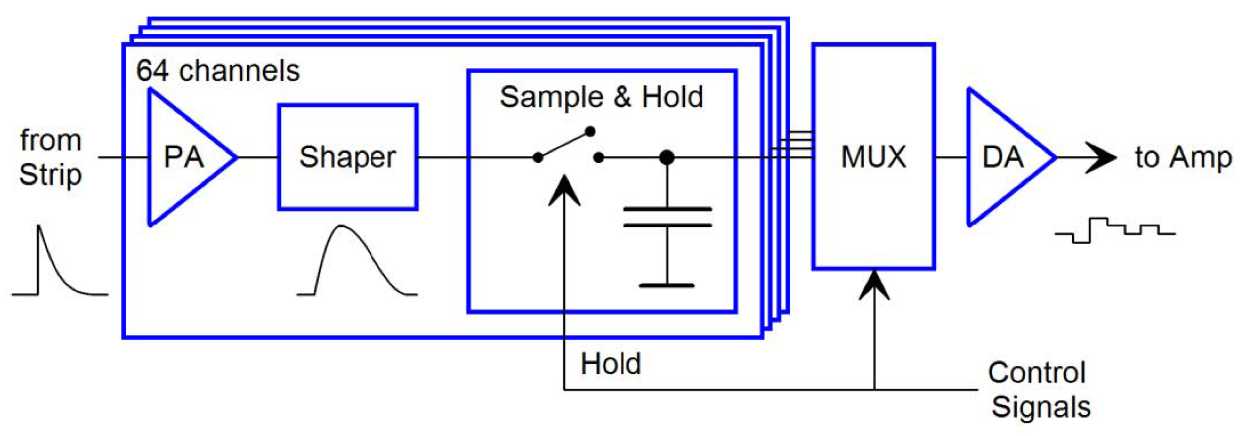
Sixteen application-specific integrated circuits (ASICs) located on the LEF, named IDE1140 or VA, read out 64 Silicon micro-strips each. Each ASIC includes an array of 64 spectrometric channels, an analog multiplexer (MUX), the registers, and the logic elements. An individual spectrometric channel contains a charge-sensitive preamplifier (PA), a shaping amplifier (Shaper), and a sample-and-hold unit. The sample-and-hold units are triggered by a common external signal (HOLD), which is generated by a field-programmable gate array (FPGA) after receiving an external trigger signal. While the HOLD signal is high, the FPGA sends 64 clock pulses to the MUX, providing the sequential readout of the signal values held in the sample-and-hold units. Then, the picked up values are amplified by an internal differential amplifier (DA) and a two- stage separate amplifier (Amp). Finally, all signals are digitized by analog-to-digital converters (ADCs). The scheme in
Figure 1 shows all the described components of the VA.
An ion beam test was performed in November 2022 at the super-proton synchrotron of CERN: A 40 mm Beryllium target was hit by a primary beam of Pb (379 GV/c), which produced ions by fragmentation. The fragments were selected magnetically, in the rigidity interval of a few percent around 300 GV/c. At this scale of rigidity, every ion is considered a minimum ionizing particle (MIP).
The Bethe–Bloch formula describes the average energy loss by a particle with charge Z that traverses a target: for a fixed
v/c and a fixed target, that quantity only depends on the charge-squared
of the incident particle. These average ionization losses are stochastic in nature, and the Bethe–Bloch formula gives the mean value of these losses: the fluctuations around this value, in thin materials, are well described by the convolution of a Gaussian and a Landauian (LanGauss) distribution [
4]. Having a beam with a population of different ions with different charges, the population distribution will be the sum of the single convolutions provided by the individual species.
2.1. Calibration and Clusterization
The ADC values of the readout strips for the
i-th channel on the
j-th VA preamplifier in the
k-th event can be written as:
where
is a constant offset pedestal (unique for each channel),
a coherent common noise component (which affects in the same way all the channels belonging to the same VA),
the strip noise, and
an eventual signal due to the passage of an ionizing particle in the depleted Silicon. The calibration procedure consists of the determination of the noise (
) for each readout channel, recording
n events in absence of incident particles (
):
To determine the noise, it is necessary to evaluate the pedestal
p and the common noise values
c. The first half part of the
n events taken establishes the preliminary values of the strip pedestals (
):
and their standard deviations:
The final values of the strip pedestals are computed using the second half of the
n events taken using:
where the ADC values
are the ones inside
with respect to
. Thanks to this procedure, the too-noisy channels for a given event are excluded from the evaluation of the pedestals. The common noise is produced by the fluctuations of the power supply and other electromagnetic interferences, and it is constant for all the preamplifiers contained in the same VA. It is evaluated event by event for each VA after subtracting the pedestal, calculating the median value. This procedure defines a valid signal by applying a threshold to the signal-to-noise ratio (S/N) of the strip:
After the calibration procedure, every channel contains two contributions: the strip noise and a possible value due to the crossing particle.
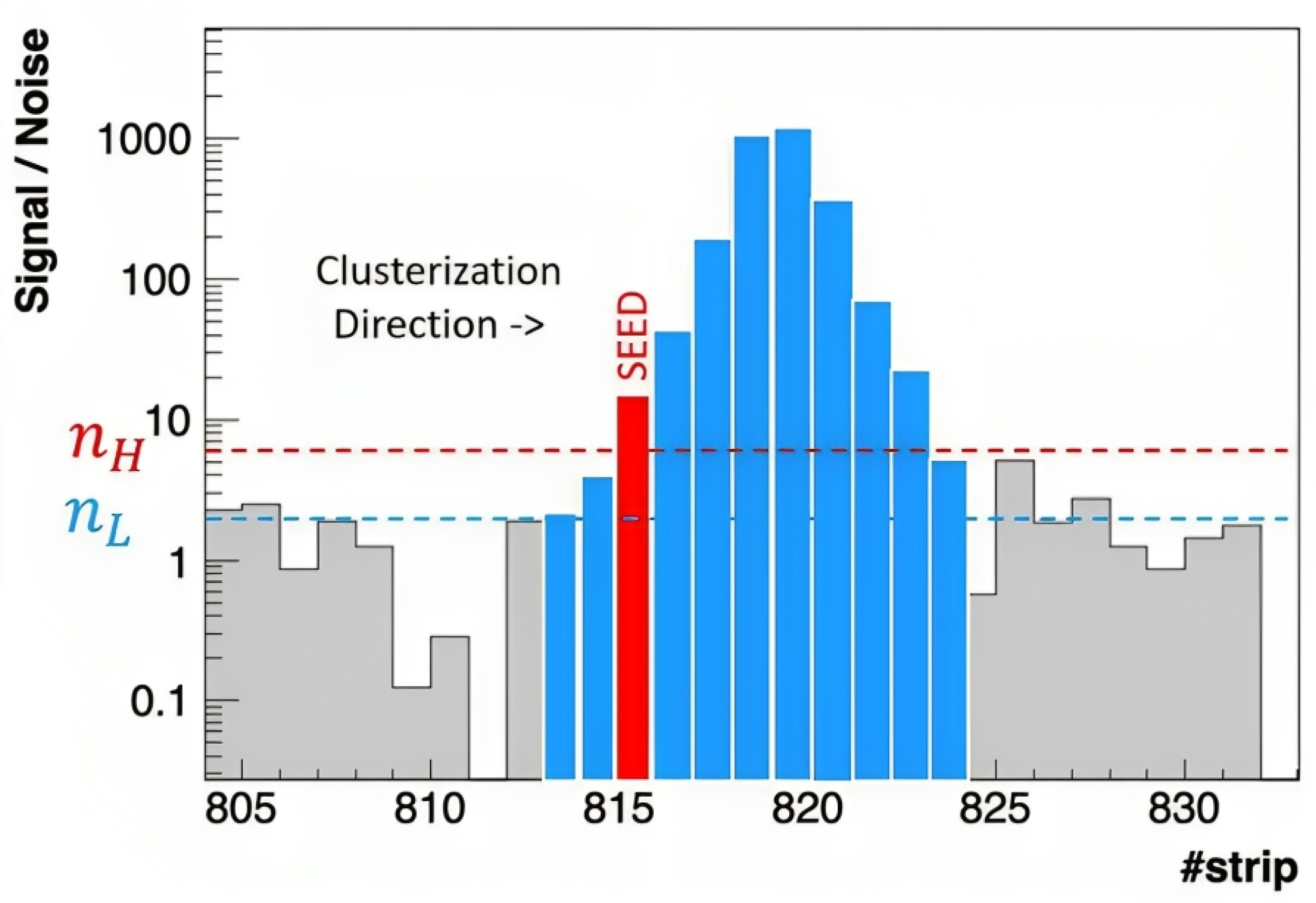
To correctly measure the charge of a crossing particle, it is necessary to identify all the strips that are interested in collecting all the released signal in the Silicon from that particle. This process is called clusterization. A cluster is a group formed by all the strips involved in the collection of the ionization energy loss by a particle. This process is performed by checking the S/N of every readout strip: The first strip found with this ratio above a certain threshold (
) is defined as the seed of the cluster. All strips adjacent to the seed are added to the cluster until their S/N ratio is above a second lower threshold (
). This procedure is performed for all 1024 readout strips of the Silicon ladder. An example is reported in
Figure 2.
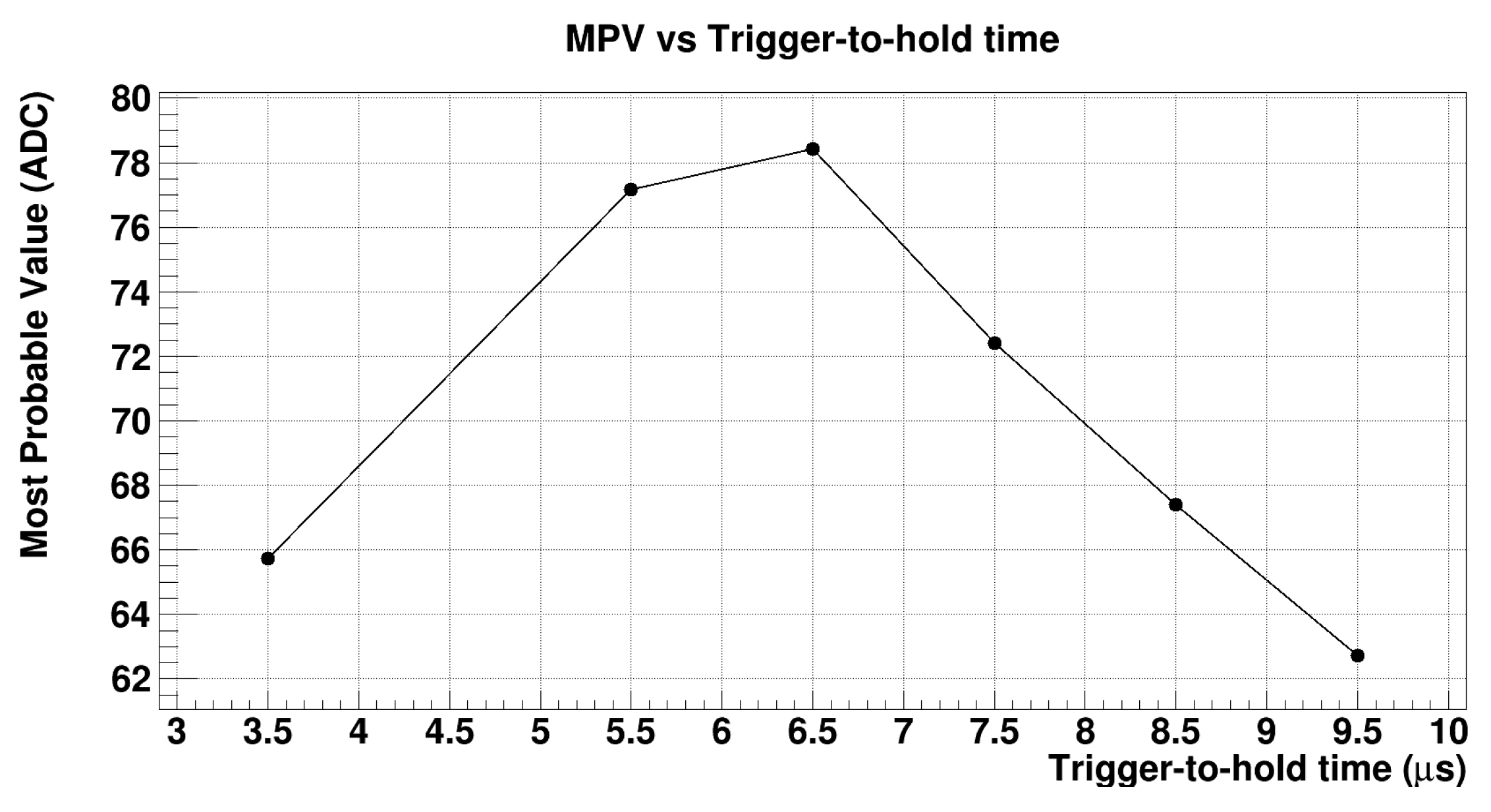
2.2. Trigger-to-Hold Time
The time, or delay, between the arrival of the external trigger and the sampling of the signal is the so-called trigger-to-hold time: waiting for the correct amount of time between these two events is a crucial point in order to sample the peak of the shaped signal. In order to find the best value for the trigger-to-hold time, a dedicated study on CERN beam test data was performed. During the data acquisition, different runs with about the same amount of data were made with different values of the trigger-to-hold time. In total, six datasets with, respectively, 3.5
s, 5.5
s, 6.5
s, 7.5
s, 8.5
s, and 9.5
s of the trigger-to-hold time were analyzed. For each dataset, the distribution of the total cluster amplitude (ADC), where the amplitude is the sum of all the contributions of all the individual cluster strips, was fit using a Landauian function. The behavior of the most-probable values extrapolated from the fits as a function of the trigger-to-hold time is shown in
Figure 3.
2.3. Eta Correction
Once all the events are clusterized, it is possible to proceed with the evaluation of the charge resolution. The dataset used for the evaluation of the charge resolution was acquired with high and low clusterization thresholds of 5.5 and 2.0, respectively, and with a trigger-to-hold time of ∼6
s. Selecting the most-energetic cluster per event, i.e., the cluster with maximum amplitude, allows a noise rejection and good cluster choosing. The considered ladder has a total of 4096 Silicon micro-strips, but only one every four adjacent strips (1024) is effectively read out by the electronics: The intermediates, called floating strips, are capacitively coupled with the readout ones. All the strips are also capacitively coupled with the metalized back plane, allowing the operation of the Silicon sensorsin overdepleted mode [
5]. This electrical scheme leads to an inter-strip energy loss. When collecting ionization, the floating strips share all the acquired signal with the nearest readout strips, but when doing this, part of the signal is lost due to the capacitive coupling with the back plane. As a first approximation, to quantify the inter-strips’ energy loss, it is sufficient to study the signal shared between the two strips closest to the particle impact position. A more-realistic description of the capacitive charge sharing has to take into account not only the direct inter-strip capacitance with the first neighboring strips, but also indirect coupling to the second and even third readouts [
6]. The inter-strips’ energy loss is quantified by
, defined as follows:
where
and
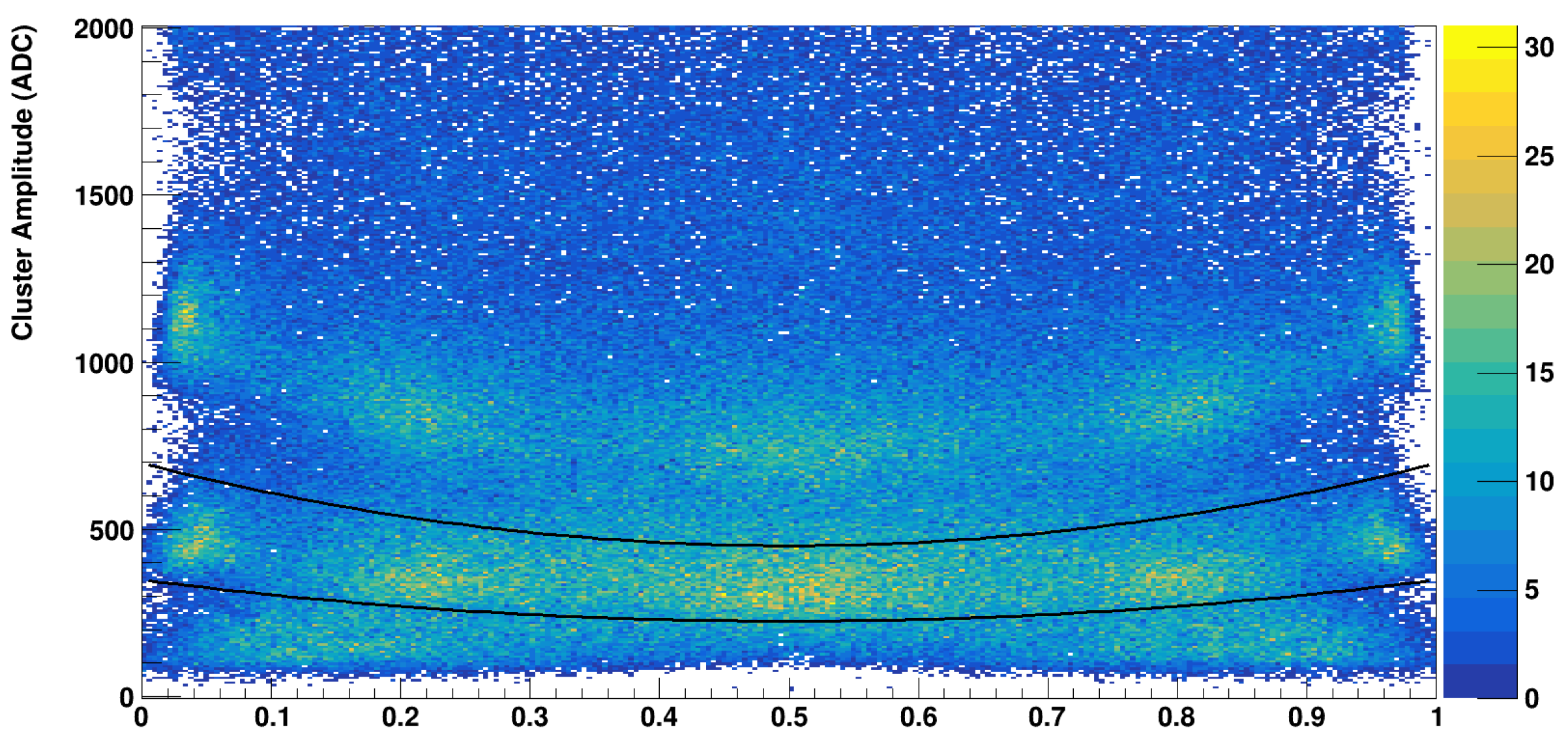
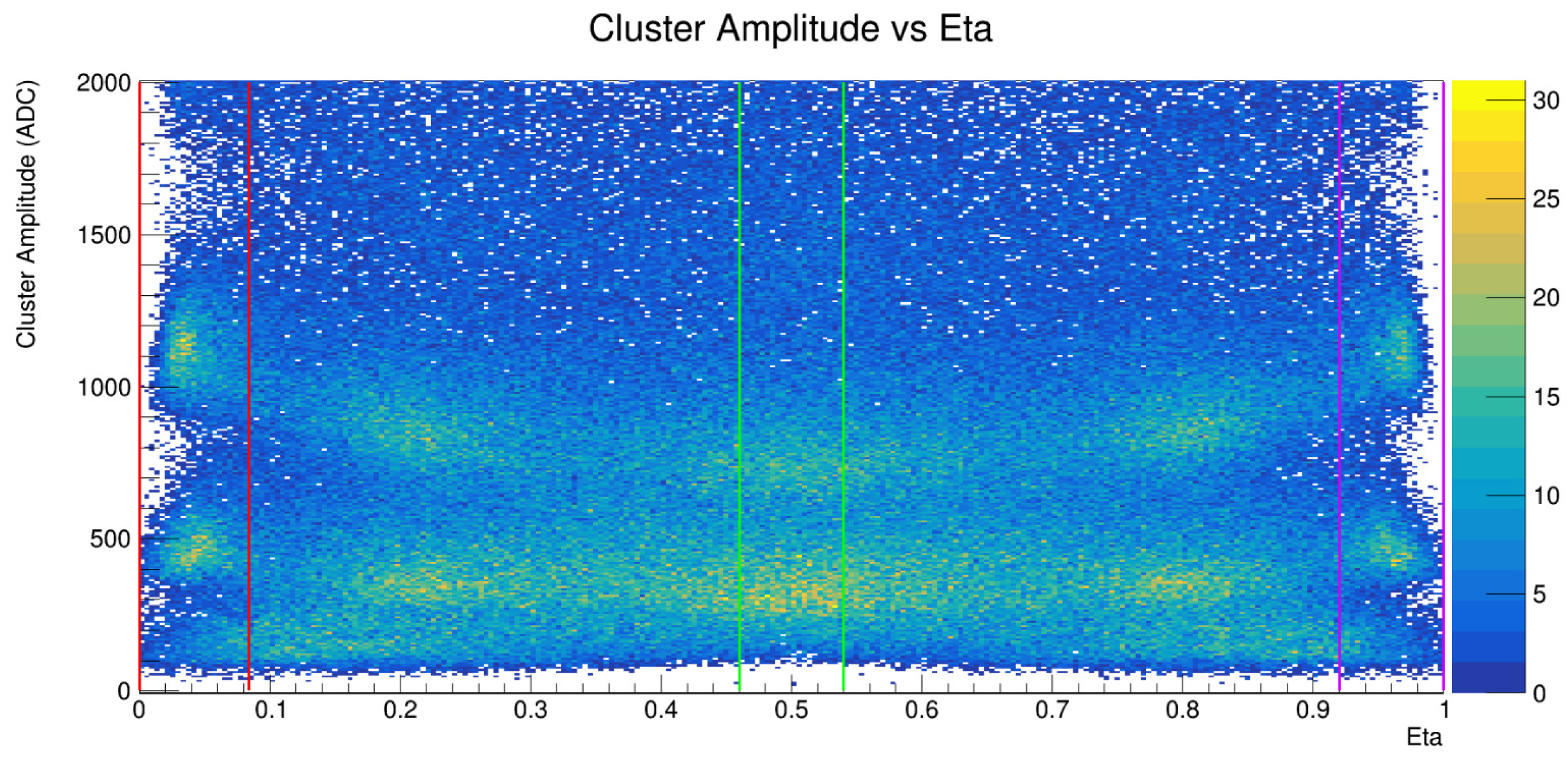
are the signals in the ADC of the two highest strips of the cluster (coinciding with the two closest to the impact position). The dependency of the total cluster amplitude on eta is shown in
Figure 4: the region between the two black lines corresponds to the energy deposited by Z = 2 particles. Different eta values, i.e., different impact positions with respect to the two highest strips of the cluster, correspond to different ADC values for the same charge. To take into account this dependency, the ADC distribution is supposed to be parabolic in eta and constant for every amplitude:
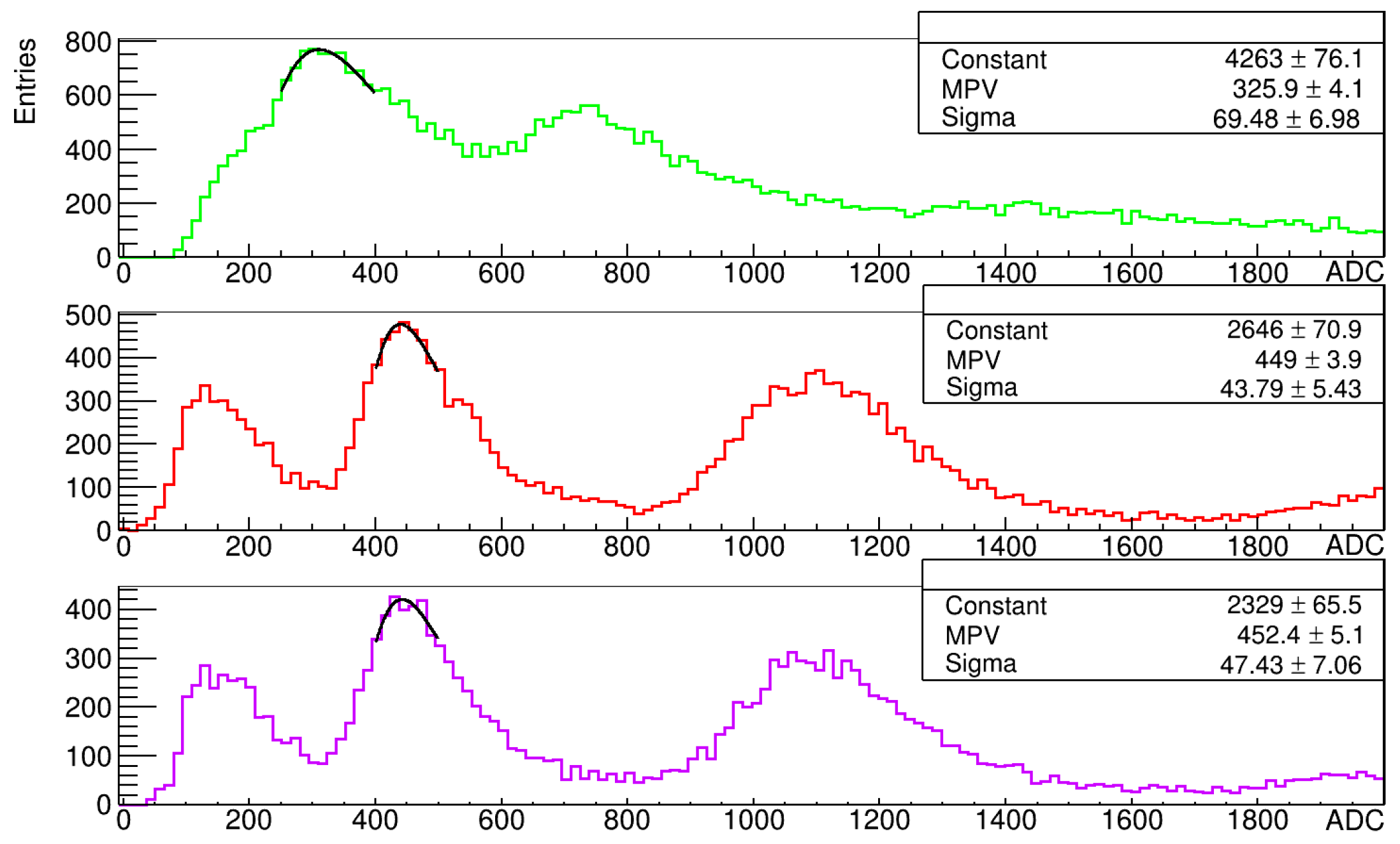
To find the coefficients of the parabola, the Z = 2 sample was used. The cluster amplitude distribution was fit with a Landauian function around the maximum, for three different eta intervals:
. The regions chosen for this purpose are shown in
Figure 5, and the fits on the Z = 2 peak for the different regions are shown in
Figure 6. The passage of the parabola was imposed on three points, each one composed of the eta values (0,0.5,1), and the most-probable values are shown in
Figure 6. The eta correction is, finally, defined as:
To get rid of the inter-strip energy loss, every ADC value was multiplied by , where c is the known term of the parabola and will be the parabola value at the eta point corresponding to the ADC value that we want to correct.
2.4. VAEqualization
Another signal correction was performed considering the VAs: ideally, one wants to observe the same response, i.e., the same ADC value, for each VA for a given Z. This did not happen, and different VAs had different response functions, which provide different ADC values for the same charges. An equalization of 9 of the 16 VAs (from Number 5 to 13) was made, considering VA Number 10 as a reference.
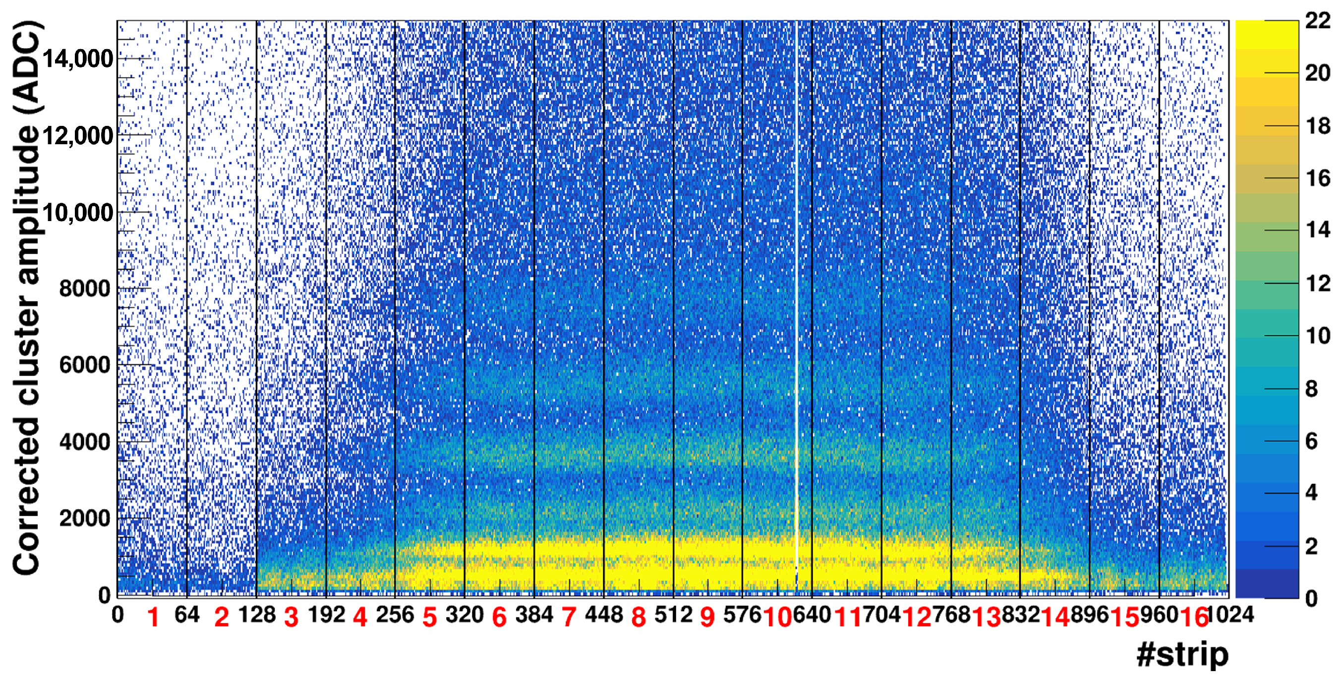
Figure 7 shows the corrected cluster amplitude distribution as a function of the strip number: in red is highlighted the VA number, going from 1 to 16. To equalize the VAs with respect to VA Number 10, the corrected cluster amplitude distribution inside a 64-channel range (which corresponds to a full VA) was studied. As mentioned, the distribution of a population containing different ions will be the sum of the single convolutions (between a Gaussian and a Landauian) provided by each ion.
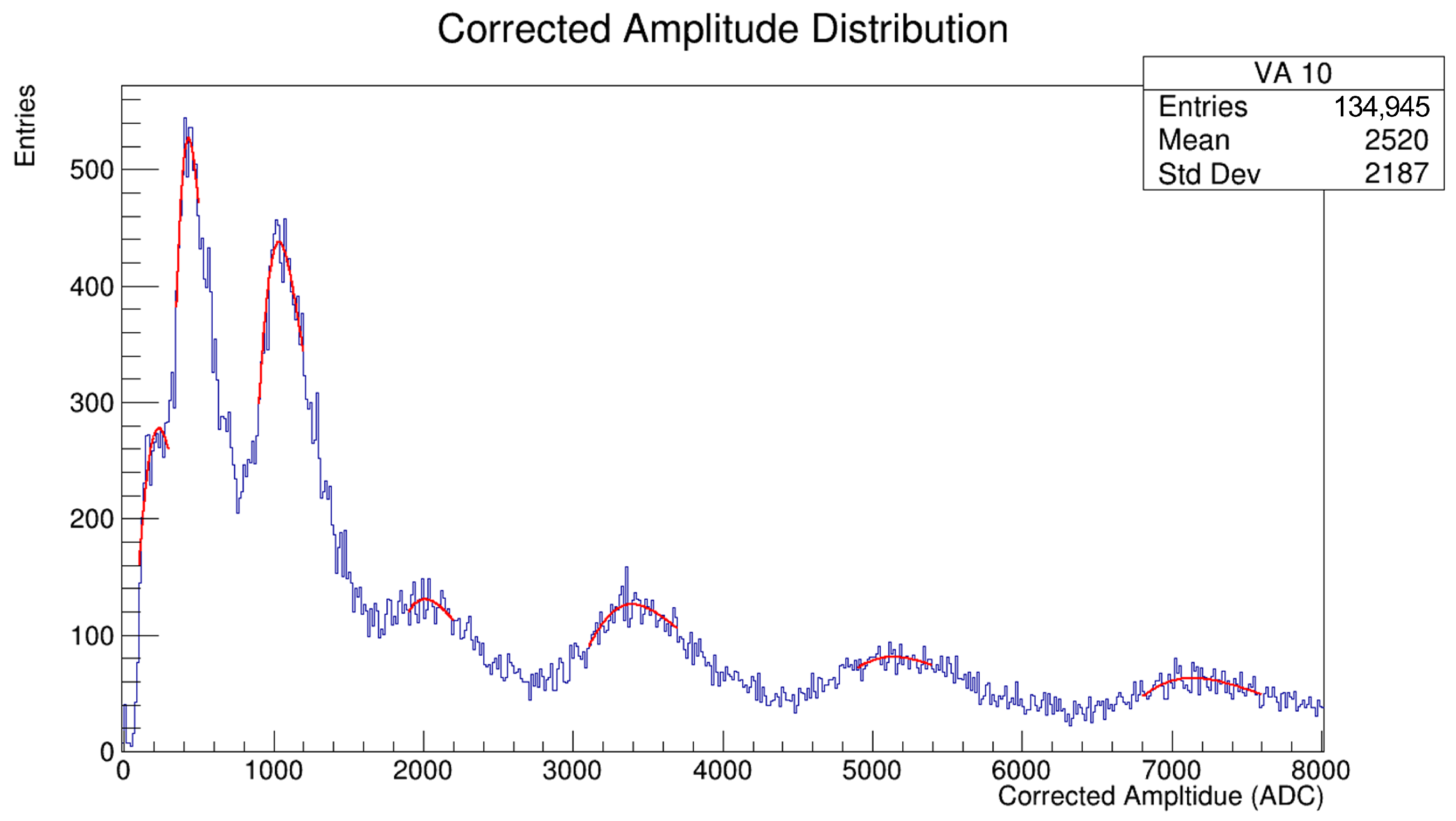
Figure 8 reports the corrected cluster amplitude distribution for VA Number 10: the red lines represent the fit performed around the peaks with the convolution between a Gaussian and a Landauian in order to estimate the most-probable values for the energy deposited by charge from Z = 2 to Z = 7. The first peak corresponds to Z = 1; despite being performed, Z = 1 was excluded from the analysis.
The same procedure was applied for the remaining eight VAs. For the
k-th VA (for a total of nine VAs from Number 5 to 13), the fits gave six most-probable values of
, with
i = 2, …, 7 and
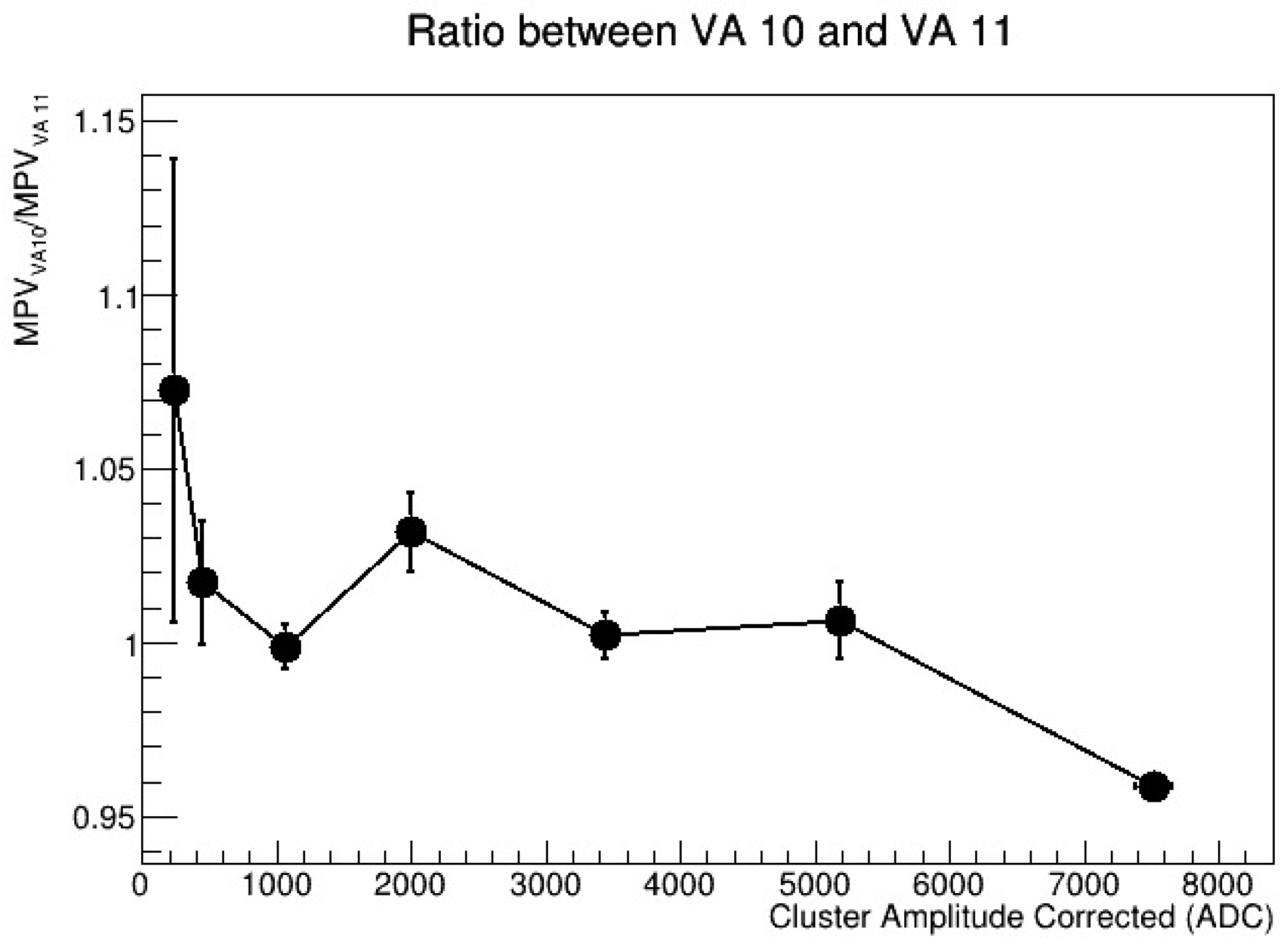
k = 5, …, 13. Then, the response functions of every VA with respect to VA 10 were built by using the ratio between the most-probable values of VA 10 (
) and the most-probable values of the remaining VAs (
) as a function of
,
k. To clarify,
Figure 9 shows the ratio between VA Number 10 and VA Number 11.
The first point corresponds to Z = 1: despite being reported, Z = 1 was excluded from the analysis because the trigger conditions were set in order to minimize the acquisition of that type of event. So, the statistics for Z = 1 is very poor and inappropriate to perform any type of statistical analysis. In reference to the same figure, the polyline that joins the points represents the function used for the equalization of VA Number 11,
. The signal measured by the k-th VA,
, was equalized with respect to VA Number 10 by:
where
is the equalization function for the k-th VA, obtained with the same procedure explained for k = 11.
2.5. Saturation
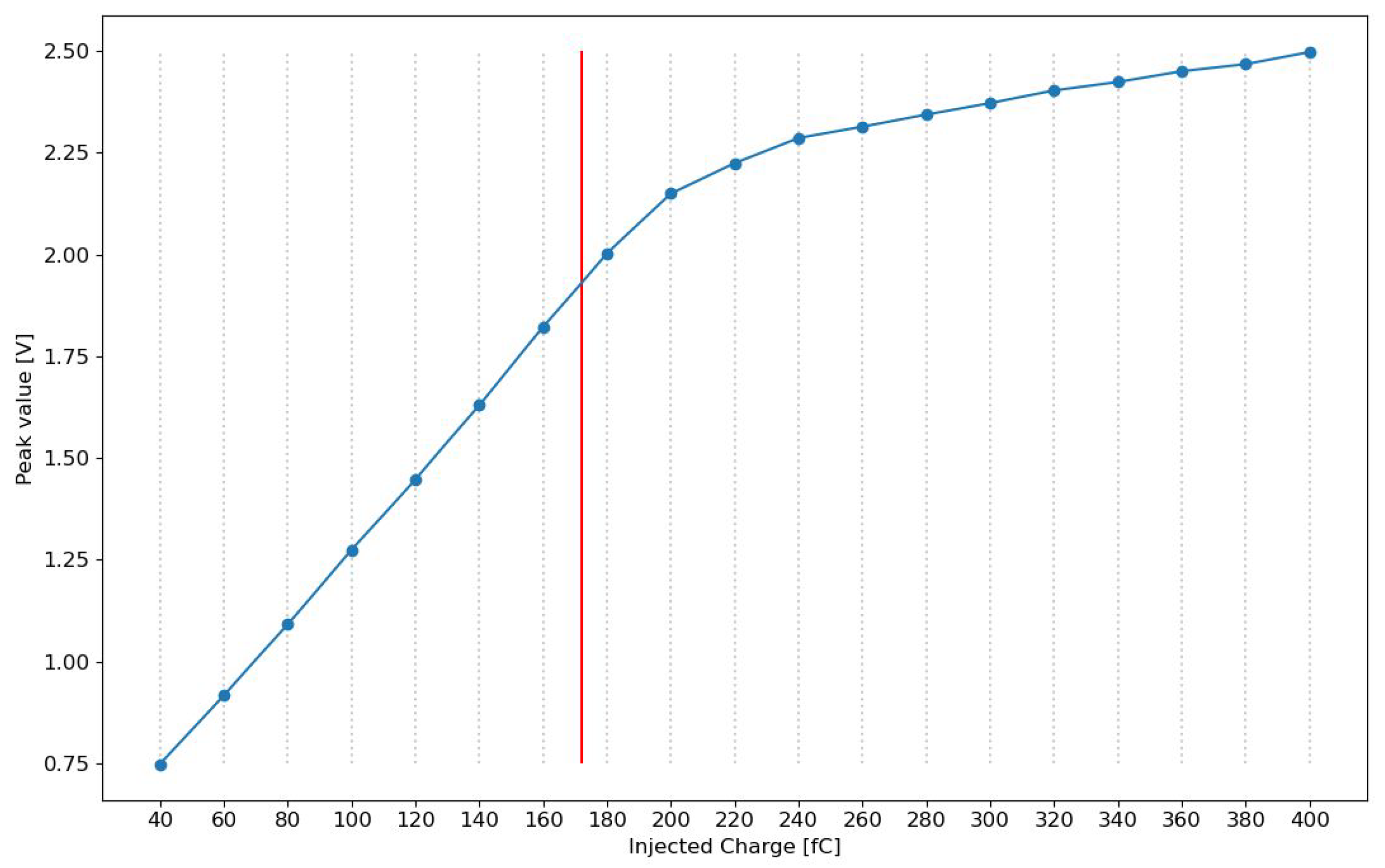
The analysis performed on the Silicon ladder was performed up to Z = 7, and it was not possible to acquire higher charges because of electronics saturation. This behavior is due to the dynamic range of the VA and the preamplifier.
Figure 10 shows the output of the VA as a function of the input signal. The VA output is a linear function of the input signal only below a certain value, that is 172 fC. As long as the input charge is below 172 fC, the VA output is linear with the charge, but above this threshold, the VA gain decreases rapidly, leading to the same output for a large range of input charges. Incident particles generate an amount of ionization and, so, a VA input that is increasing with Z
2: the non-linear behavior of the VA for high charges limited the analysis to only those charges with Z ≤ 7.
2.6. Charge Resolution
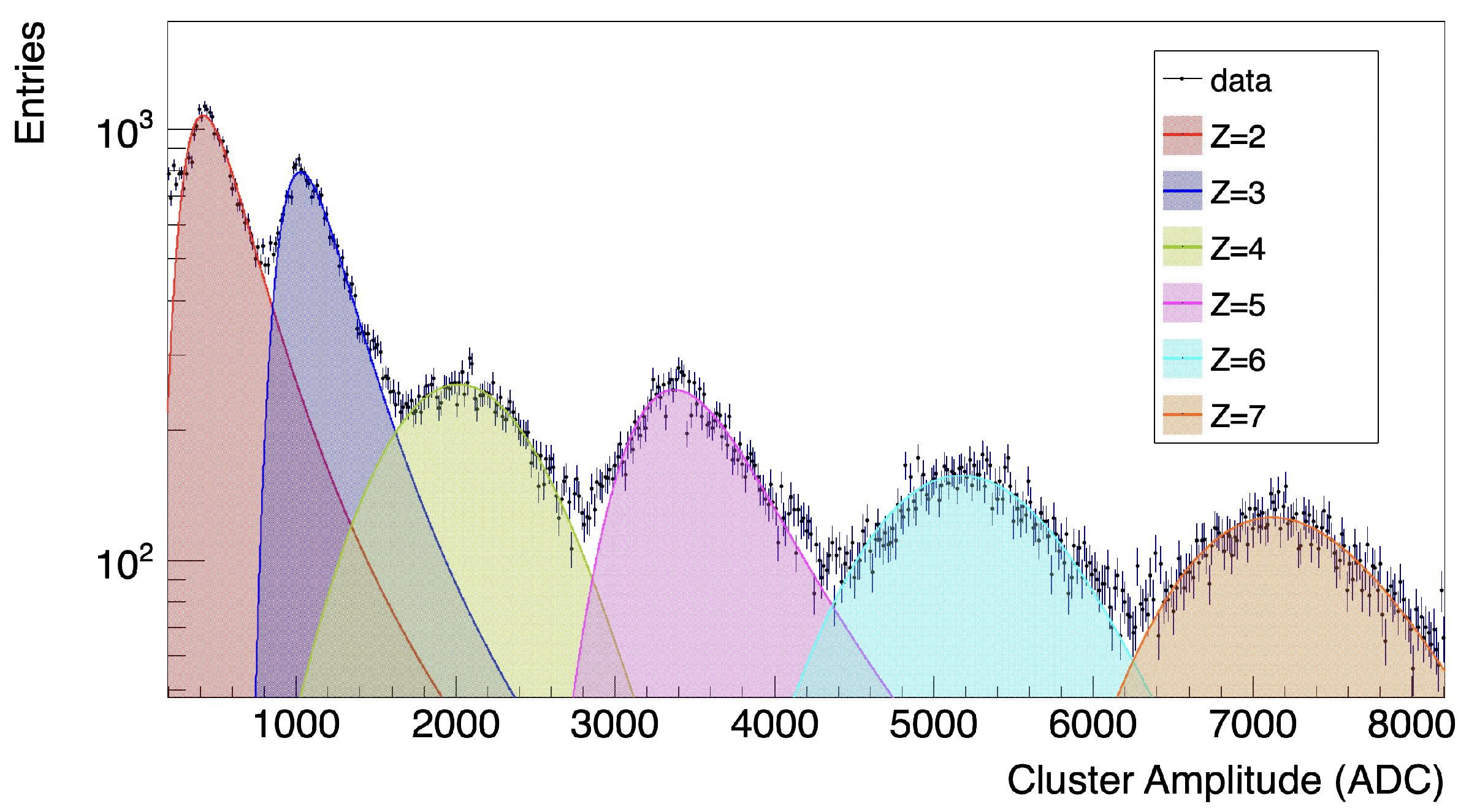
Figure 11 shows the distribution of the total cluster amplitude corrected by eta and equalized with respect to VA Number 10 and the six convolution functions used to fit that distribution. The applied procedure to measure the final charge resolution was the following:
The total cluster amplitude corrected by eta and equalized with respect to VA Number 10 was fit with six different LanGauss functions;
The parameters obtained from the fits were used to generate a Monte Carlo (MC) toy for each charge sample by the square root of a random event generated using the probability density functions (PDFs). Thanks to the Bethe–Bloch formula, the mean energy loss by a particle was proportional to Z2, which was measured by the detector in ADC counts. In order to evaluate Z, it was necessary to study the distribution;
The MC toy was used to apply the central limit theorem (CLT) to estimate the charge resolution.
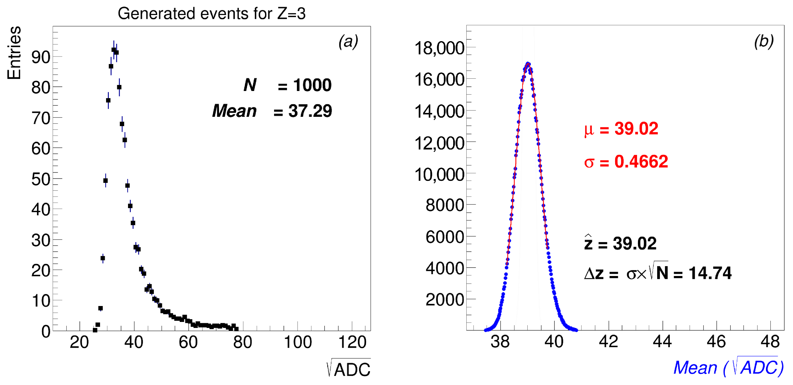
The PDFs with i = 2, …, 7, were built. A sample of N = 1000 events for the i-th charge was generated by the square root of a random event created using .
As an example, in
Figure 12a is reported the
distribution for Z = 3 and its arithmetic mean generated with the MC toy. The
distribution reported in the same figure follows a PDF,
, with an expectation value of
and variance
. The resolution of the charge will be
.
According to the central limit theorem (CLT), for a variable x with expectation value E[x] =
and variance V[x] =
, the distribution of the mean is Gaussian with mean
and variance
linked to
and
by:
Figure 12b shows the mean distribution for Z = 3 for M =
Monte Carlo experiments (each one with N = 1000 events): it is possible to evaluate
as the mean of the Gaussian distribution and
as
.
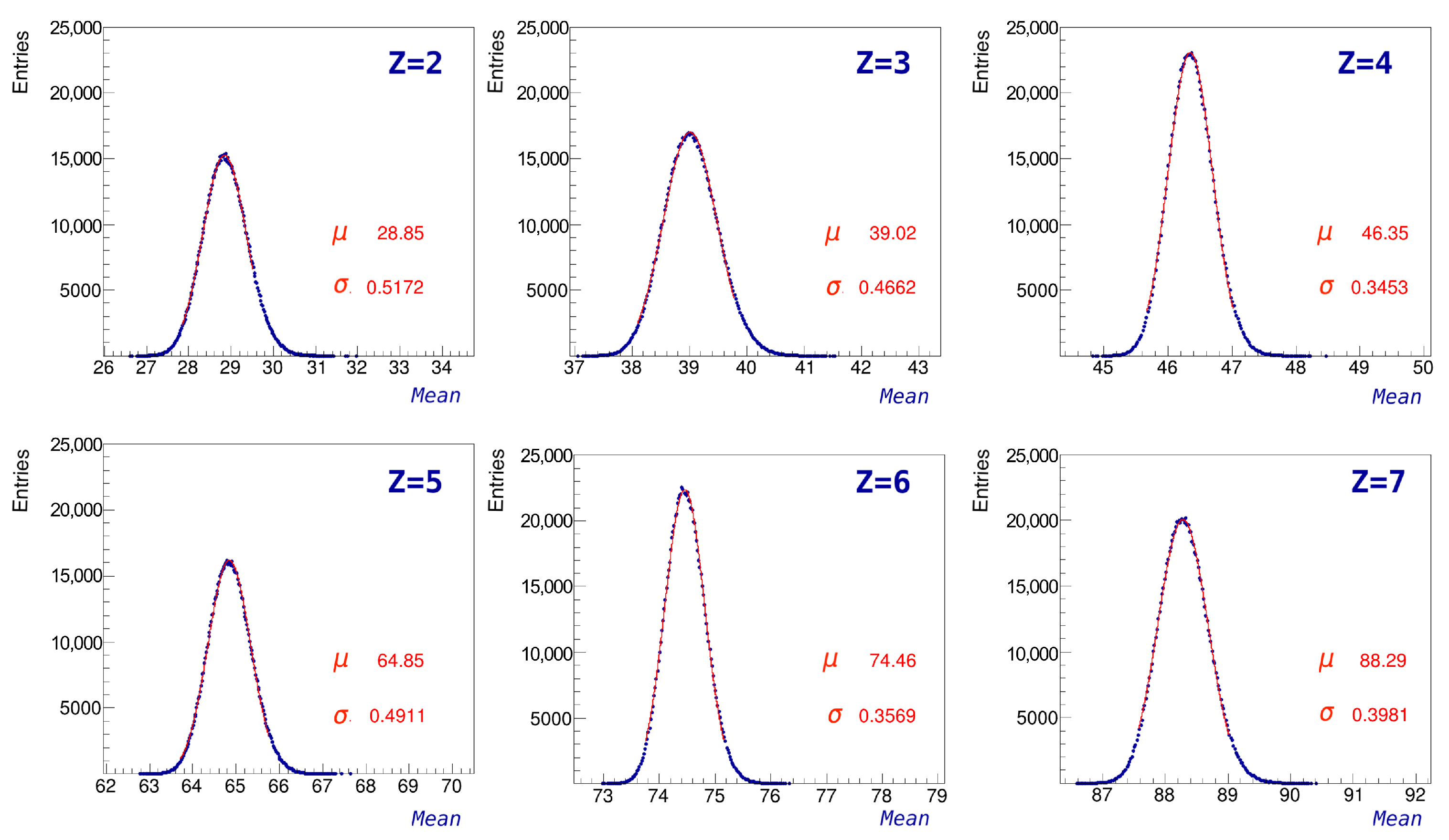
Figure 13 shows the distributions of the means for all the charges under study (from Z = 2 to Z = 7) and the relative Gaussian fit with mean
and standard deviation
.
4. Discussion
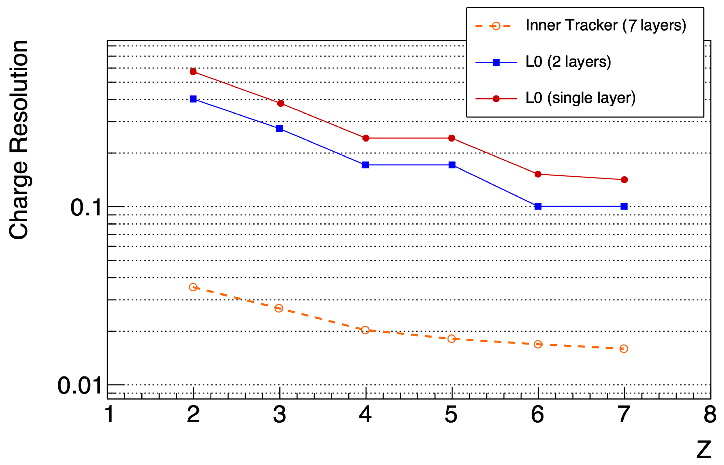
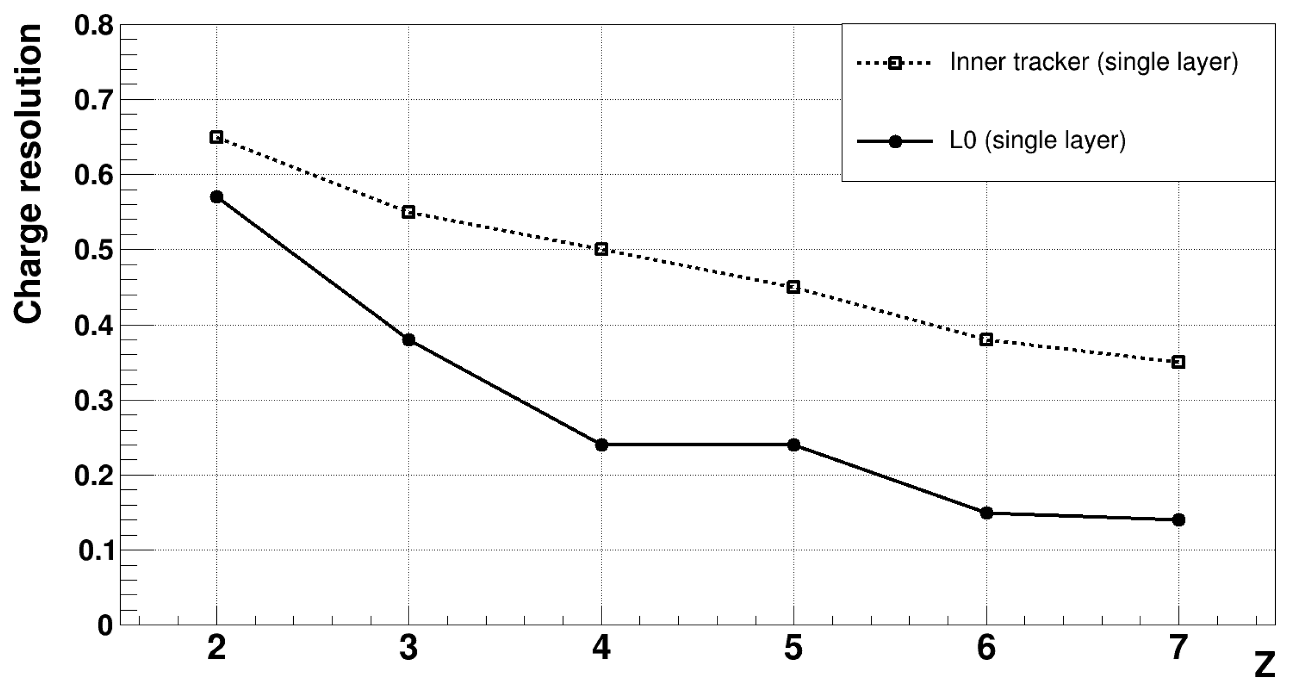
The study performed on the Silicon AMS-02 Layer 0 prototype showed agreement in terms of the charge resolution with respect to the AMS-02 inner tracker. The signal collected by the Silicon sensors was analyzed after the calibration to find an algorithm that allows discriminating the signal from the noise. After the selection of the signal, an accurate characterization of the signal released by different species was performed with 2 ≤ Z ≤ 7 in the Silicon sensors that will be used for the construction of L0. In the current state, the new layer on top of AMS-02 will be able to measure the charge at least up to Z = 7 with a resolution of 10%.
The obtained resolutions can be further improved. For example, the lack of statistics for Z = 1, due to trigger conditions, can be compensated by future data acquired with a suitable setup to maximize the Z = 1 particles’ acquisition.
Furthermore, the applied correction for can be improved considering the different dependencies for different charges.
Moreover, the saturation of the electronics (VA) limited the acquisition of high charges to Z = 7. Indeed, considering that the analog-to-digital converter has an input range of V (the full scale equals ADC = 16 383 ADC), this is consistent with the fact that saturation appeared at a VA output value of 2 V, which corresponds approximately to 8000 ADC. By investigating the dynamic range of the VA itself and by studying the various amplify stages, it will be possible to study even higher charges.
Moreover, other improvements would be possible considering the fits performed on the cluster distribution of
Figure 11: in the current state, every contribution has been fit with a single LanGauss function described by five parameters, for a total of six different LanGauss functions. The fit could be improved by using a single function constituted by the sum of six LanGauss functions, which could possibly be more accurate.


