Real-Time Monitoring of Solar Energetic Particles Using the Alpha Magnetic Spectrometer on the International Space Station

Abstract

The International Space Station (ISS) orbits at an average altitude of 400 km, in the Low Earth Orbit (LEO) and is regularly occupied by astronauts. The material of the Station, the residual atmosphere and the geomagnetic field offer a partial protection against the cosmic radiation to the crew and the equipment. The solar activity can cause sporadic bursts of particles with energies between ∼10 keV and several GeVs called Solar Energetic Particles (SEPs). SEP emissions can last for hours or even days and can represent an actual risk for ISS occupants and equipment. The Alpha Magnetic Spectrometer (AMS) was installed on the ISS in 2011 and is expected to take data until the decommissioning of the Station itself. The instrument detects cosmic rays continuously and can also be used to monitor SEPs in real-time. A detection algorithm developed for the monitoring measures temporary increases in the trigger rates of AMS, using McIlwain’s L-parameter to characterize different conditions of the data-taking environment. A real-time monitor for SEPs has been realized reading data from the AMS Monitoring Interface (AMI) database and processing them using the custom algorithm that was developed.

1. Introduction

The International Space Station (ISS) orbits at an average altitude of about 400 km, in the Low-Earth Orbit (LEO) and is exposed to a flux of Cosmic Rays (CRs), i.e., energetic particles that wander around in the universe and which can enter into our Solar System. Equipment and crew members inside the ISS are partially shielded from the cosmic radiation by the surrounding material of the station itself, the residual atmosphere and the geomagnetic field.

CRs are mainly injected by galactic and extra-galactic sources [1]; however, the solar activity itself produces a flux of energetic particles, which affects the CR spectrum observed from Earth. The Sun ejects a flow of plasma into the interplanetary space, the Solar Wind (SW), which influences the CR energetic spectrum. In addition, violent phenomena taking place on the surface of the Sun (e.g. reconnection of magnetic field lines; Coronal Mass Ejections (CMEs)) can eject bursts of energetic particles, Solar Energetic Particles (SEPs), into space, with energies ranging from ∼10 keV and several GeVs. SEP events can last for hours or even days and are primarily composed by protons [2,3].

The ISS is not completely shielded from cosmic radiation and, during extra-vehicular activities, the exposure is high. Therefore, the radiation hazard that astronauts are subjected to has to be monitored.

The Alpha Magnetic Spectrometer 02 (AMS-02) is installed on one of the side arms of the ISS and measures the CR flux continuously [4]. The instrument is composed of different detectors to measure the characteristics of passing particles: a Silicon Tracker, to measure the rigidity and particle charge sign; a Time-of-Flight (ToF), to measure the velocity, the moving direction and the particle charge magnitude Z; a Transition Radiation Detector (TRD), to identify and separate $e^{\pm }$ from p and nuclei; a Ring Imaging Cherenkov (RICH), to measure the velocity and Z; and an electromagnetic calorimeter (ECAL), to measure the energy. Due to its equipment, AMS-02 is also suitable for detecting SEPs. In particular, ongoing SEP events can be detected by looking for sudden increments of the trigger rates [5]. The low latency of the trigger system allows for building an effective real-time monitor for SEP fluxes affecting the ISS, which could also be used to alert the astronauts onboard.

2. Materials and Methods

Intense SEP fluxes increase AMS trigger rates above the usual averages. This feature can be used to detect and monitor ongoing SEP events [5].

The AMS Monitoring Interface (AMI) contains all the data needed to monitor SEPs [6]. The AMI is made of InfluxDB databases to store the data and Grafana instances to visualize them. The monitor described in this manuscript adopts an architecture similar to the one used for the AMI. First, a series of fillers processes AMI data, utilizing a custom algorithm developed for this work [7]. Then, the fillers results are written in an InfluxDB database, connected in turn to a Grafana instance, which acts as an interface for SEP monitoring [8].

2.1. Primary Data

The AMI database is written by a feeder that recurrently processes the raw data flow of AMS directly on board the ISS. Data writing occurs approximately every minute when the connection to the ground is available. When the connection is lost, scientific data are buffered until it is re-established, usually within 20–30 min.

The delays in the writing operations and the interruptions of the data flow from the ISS can decrease the number of entries found in real-time in the AMI database. To prevent data losses in the SEP monitor, the AMI database is queried multiple times, first in real-time and then with different delays, at intervals of 30 s, 1 min, 2 min, 5 min, and 1 h.

The analysis algorithm uses AMS trigger rates and live-time to search for increases in the instrument activity that could be due to an SEP event. In addition, ISS positions and flight angles are also used to calculate the geomagnetic field intensity, the zenith angle and the McIlwain’s L-parameter [9], useful for characterizing the impact of the geomagnetic field on the data. To avoid the use of outdated information, records with positions or flight angles updated respectively more than 10 s or 1 min before are discarded.

2.2. AMS-02 Trigger Rates

AMS-02 uses two types of triggers: fast triggers (FTs) and level-1 (LV1) triggers [10]. FTs are evaluated in ∼40 ns, while LV1 triggers can take up to 1 $\mathsf{\mu }$s and are evaluated only in the case of a positive FT. Fast trigger is in turn the logical OR of other three signals:

• Fast Trigger Charged (FTC), which evaluates the possible presence of events with charged particles;
• Fast Trigger big-Z (FTZ), which evaluates the possible presence of events with highly-charged particles;
• Fast Trigger ECAL (FTE), which evaluates the possible presence of events with electromagnetic interactions in the ECAL.

On the other hand, the LV1 trigger can compose up to 8 sub-level-1 (subLV1) triggers; currently only 7 are defined and used:

0

unbiased trigger for events with charged particles;

1

trigger for events with single charged particles;

2

trigger for events with normal ions;

3

trigger for events with slow ions;

4

trigger for events with electrons;

5

trigger for events with photons;

6

unbiased trigger for events with electromagnetic interactions.

The fast and LV1 triggers make use of signals from the ToF, the ACC and the ECAL.

The SEP monitor takes into consideration all the trigger rates, except for subLV1-6, which has an extremely low rate.

The status of the trigger is monitored in AMS by scalers placed in the LVL1 board that count how many times each trigger condition has been fired during the previous second. At the same time, the board measures the experiment live-time, i.e., the fraction of the previous second during which the detector was available for data acquisition.

Because of the dead-time of the instrument, measured trigger rates ${\lambda }_{\mathrm{meas}}$ need to be adjusted to their true values $\lambda$, dividing them by the live-time $\eta$:

$$\lambda ={\lambda }_{\mathrm{meas}}/\eta .$$

(1)

In our study we measure trigger rates in 1-min time interval. The rates corrected by the live-time are of the order of 100–1000 Hz.

A special case occurs for trigger rates that are generally low, i.e., ≲10 Hz. For those, the rate distribution can be discrete and simply dividing by the live-time would be inadequate to get the true rate. Because of that, in this work all the measured trigger rates are corrected by the live-time, except for FTZ and subLV1-3. In the Supplemental Materials the live-time and the trigger rates distributions are shown in detail.

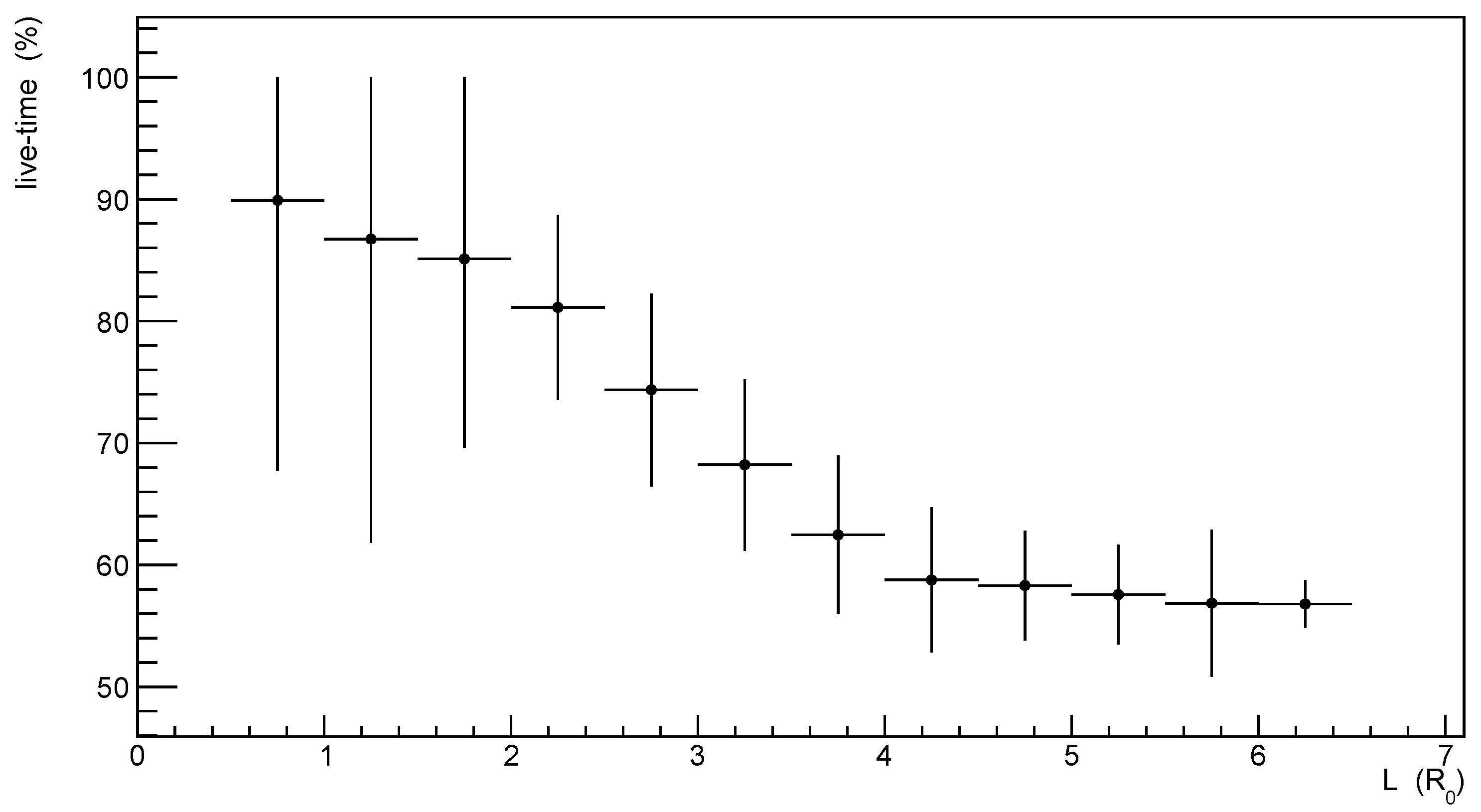
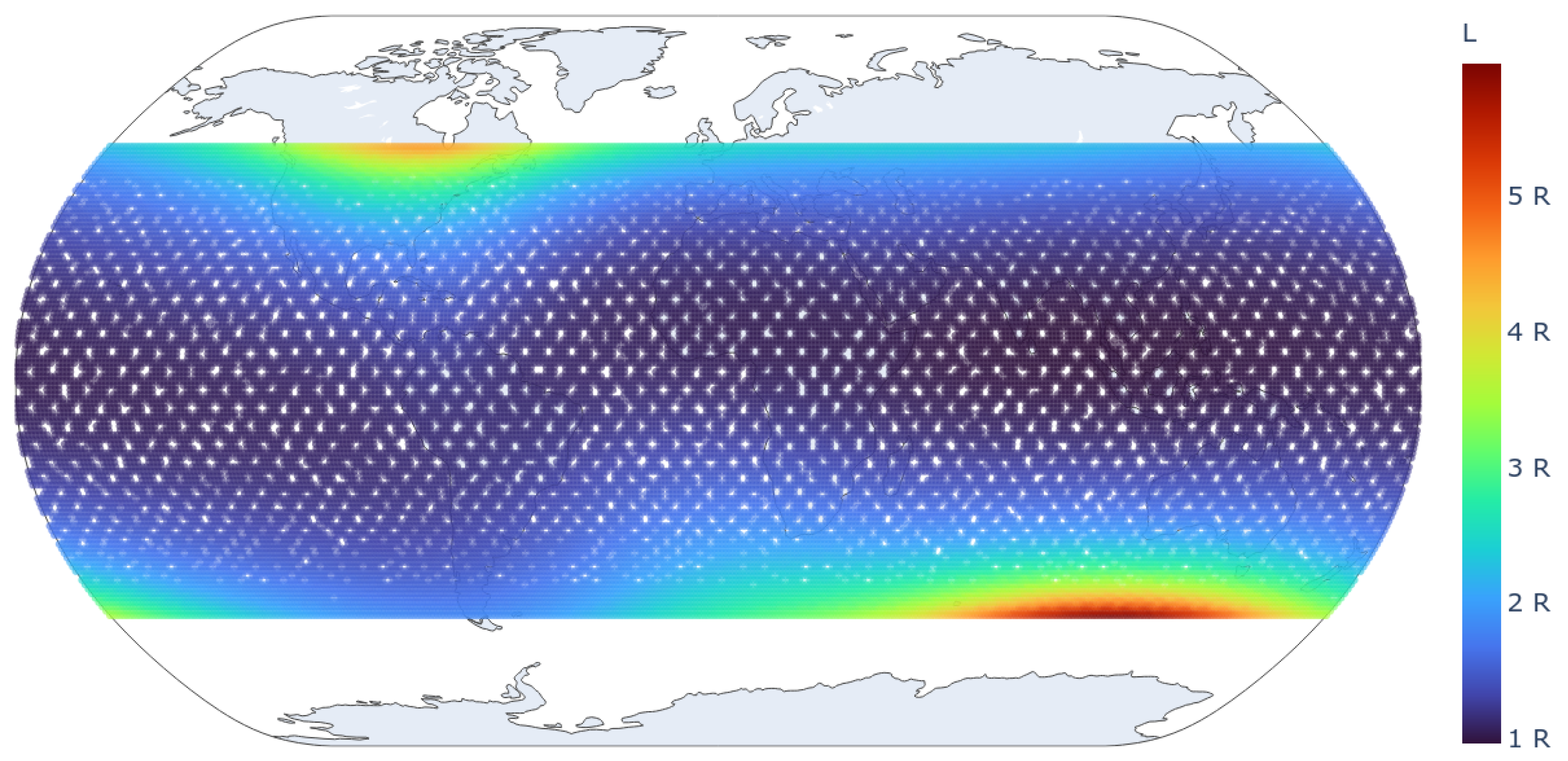
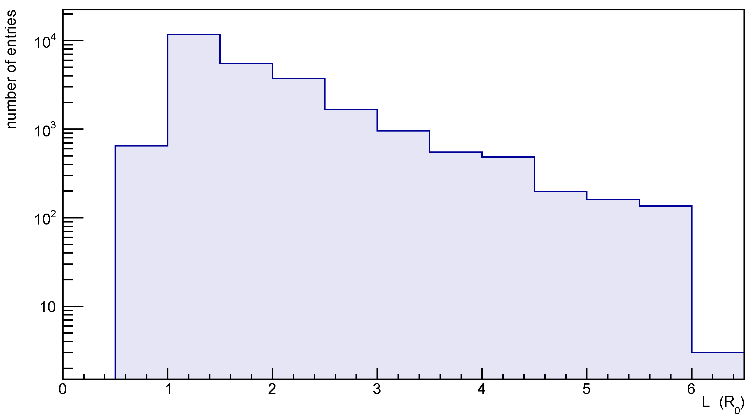
2.3. Impact of the Geomagnetic Field

The nominal level of a trigger rate varies along the ISS orbits. The particle flux observed on satellites in LEO is strongly influenced by the geomagnetic environment, which permits only particles with a rigidity greater than the local cutoff. Cutoff rigidity can be determined by tracing particles of different energies in the magnetosphere and depends on the satellite location and particle direction. Figure 1 illustrates how AMS activity varies in function of McIlwain’s L-parameter, which is a convenient parameter to describe the cutoff rigidity for a particle entering from the zenithal direction, as a function of the satellite position in the geomagnetic field [9].

The relationship between the L-parameter and the vertical cutoff rigidity $R_{\mathrm{VC}}$ is shown by the equation

$$L=\sqrt{k/R_{\mathrm{VC}}},$$

(2)

with $k\simeq 16.2\mathrm{GV}·R_0^2$ and $R_0$ the Earth radius [11]. Figure 2 shows a map of the L-values calculated for 1 month of ISS orbit data.

The ISS orbits project onto the Earth’s surface within a latitude range spanning from approximately $-{52}^{\circ }$ to $+{52}^{\circ }$. Within this range, the motion of the ISS does not entirely cover the Earth’s surface, as evident from the lack of data points in the central region of the map depicted in Figure 2. Furthermore, Figure 2 reveals that the majority of the path traversed by the ISS is associated with low L-values, typically less than 3 $R_0$. However, as the ISS approaches the poles, the L-parameter can reach higher values, peaking at around 6 $R_0$. Higher L-values correspond to lower vertical cutoff rigidities, expanding the potential for observing SEP events with lower energy levels.

For this work, trigger rate distributions are grouped in fixed bins of L from 0 to 6.5 $R_0$, 0.5 $R_0$ wide. Figure 3 shows the statistics that characterizes the defined L bins.

Due to the non-perfect dipolar shape of the geomagnetic field, the field lines come closer to the Earth’s surface in correspondence of the South Atlantic Anomaly (SAA), a region where particles trapped in the Van Allen belts cross the satellite orbit. This feature causes an observed higher flux, with a variability dependent on how the SAA is crossed by the ISS. Those increments are not related to a possible SEP event, therefore these regions are excluded from further analysis imposing a lower threshold of 25,000 nT on the geomagnetic field intensity. The intensities are obtained from the GPS positions, using the 13th generation of the International Geomagnetic Reference Field (IGRF) [12].

Another situation where AMS could experience a sudden change in the number of detected particles is when the ISS flight orientation is changed significantly, e.g., during the docking of a spacecraft. In those cases, AMS might assume a great inclination with respect to the zenith axis. ISS flight angles, i.e., yaw, pitch and roll can be used to calculate the zenith angle of AMS. To exclude increments of the trigger rates related to fluxes of particles trapped along the geomagnetic field lines, data collected with a zenith angle greater than ${15}^{\circ }$ are discarded.

2.4. Detection of SEPs

An SEP event can increase AMS trigger rates over their usual levels observed in a specific geomagnetic region. To quantify the increments, a score s is defined and assigned to each data entry:

$$s={\int }_{\overline{\lambda }}^{+\infty }f(\lambda ;\mu ,\left[\sigma \right])\mathrm{d}\lambda ,$$

(3)

with $\overline{\lambda }$ representing the observed trigger rate, f the PDF that models its distribution, and $\mu$, $\sigma$ respectively the average and the standard deviation of rates from the preceding 3 days; $\sigma$ is actually an optional parameter, used only when f is a continuous function. Regarding the time window used for assessing $\mu$ and $\sigma$, the ISS orbit around the Earth takes ∼90 min and its precession ∼16 orbits; therefore, the window spans ∼3 ISS motion cycles. The trigger rates corrected by live-time are modeled by a Gaussian distribution, while the lower-rate ones, not corrected by the live-time (i.e., FTZ and subLV1-3), are modeled by a Poisson distribution.

Time-series of $\mu$ and $\sigma$ show a step trend that can lead to apparent increments in the score calculus, when L is about to change its bin. In order to remove this effect, $\mu$ and $\sigma$ are smoothed using the linear interpolation between the values obtained from the two closest bins.

The score defined in Equation (3) is eventually used to detect the presence of an SEP event. Specifically, increments in the trigger rates resulting from intense SEPs would lead to low score values, tending to 0. Because of its definition, the score value can also be seen as the p-value of the observed increment to be outcome of just a statistical fluctuation. This perspective is valuable for establishing a cut for the scores to avoid biasing the reference distributions defining the trigger rates nominal levels. Indeed, data with a score smaller than ${10}^{-6}$ are excluded from entering the 3-days time window, eliminating ∼2 entries per year due to statistical fluctuations.

3. Results

The real-time SEP monitor resulting from the work described in this manuscript is published at [8]. AMI data are analyzed in real-time and again after 30 s, 1, 2, 5 min, and 1 h. Real-time fillers are kept running on a separate deployment platform and the results are stored in an InfluxDB database to which the Grafana interface is connected.

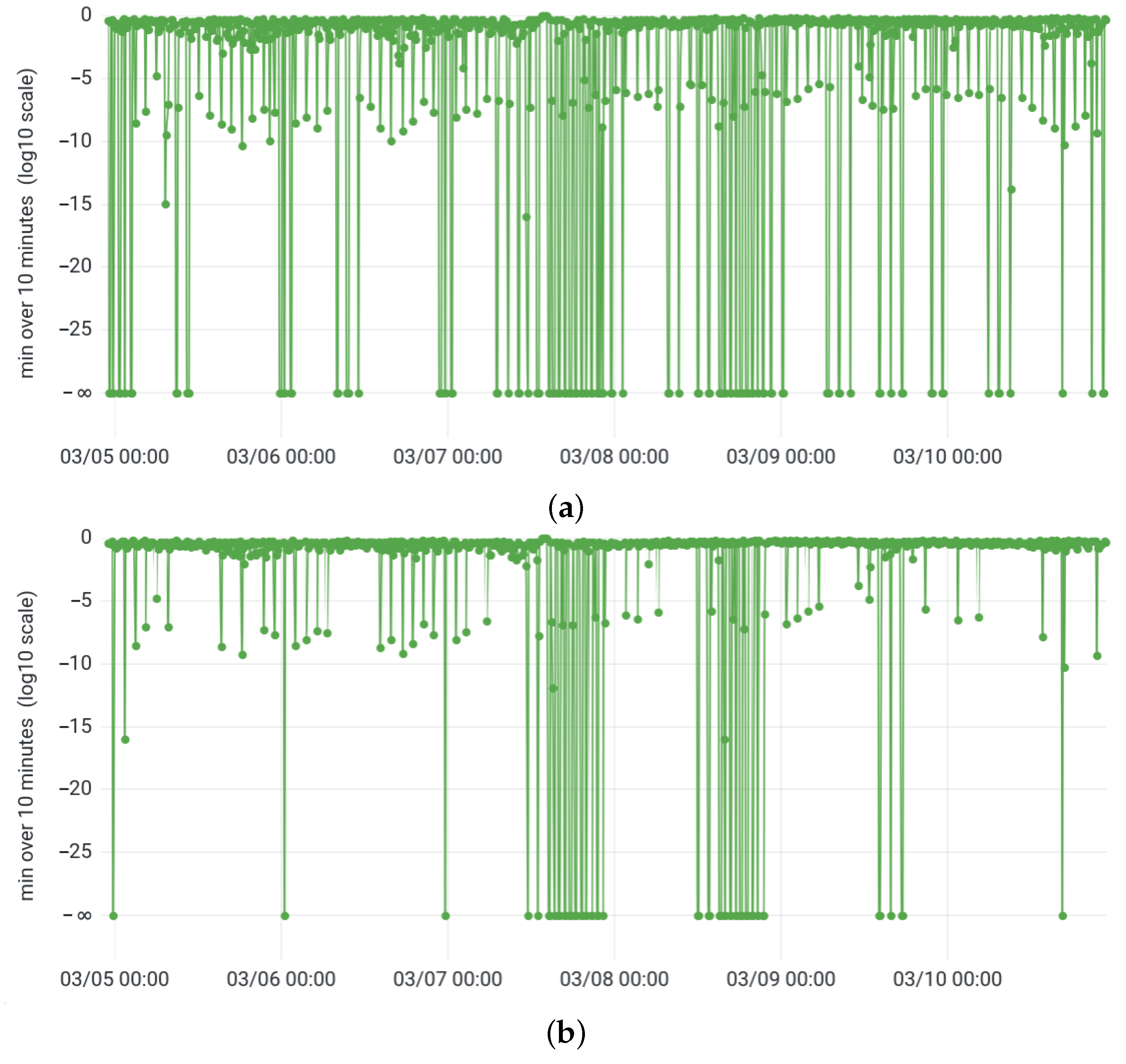
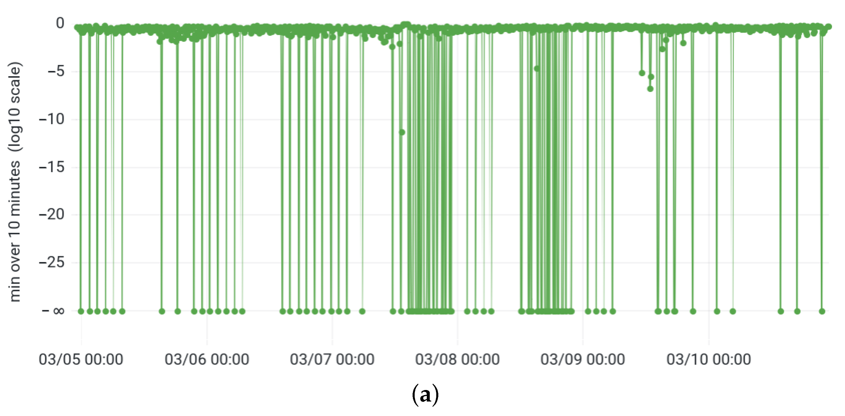
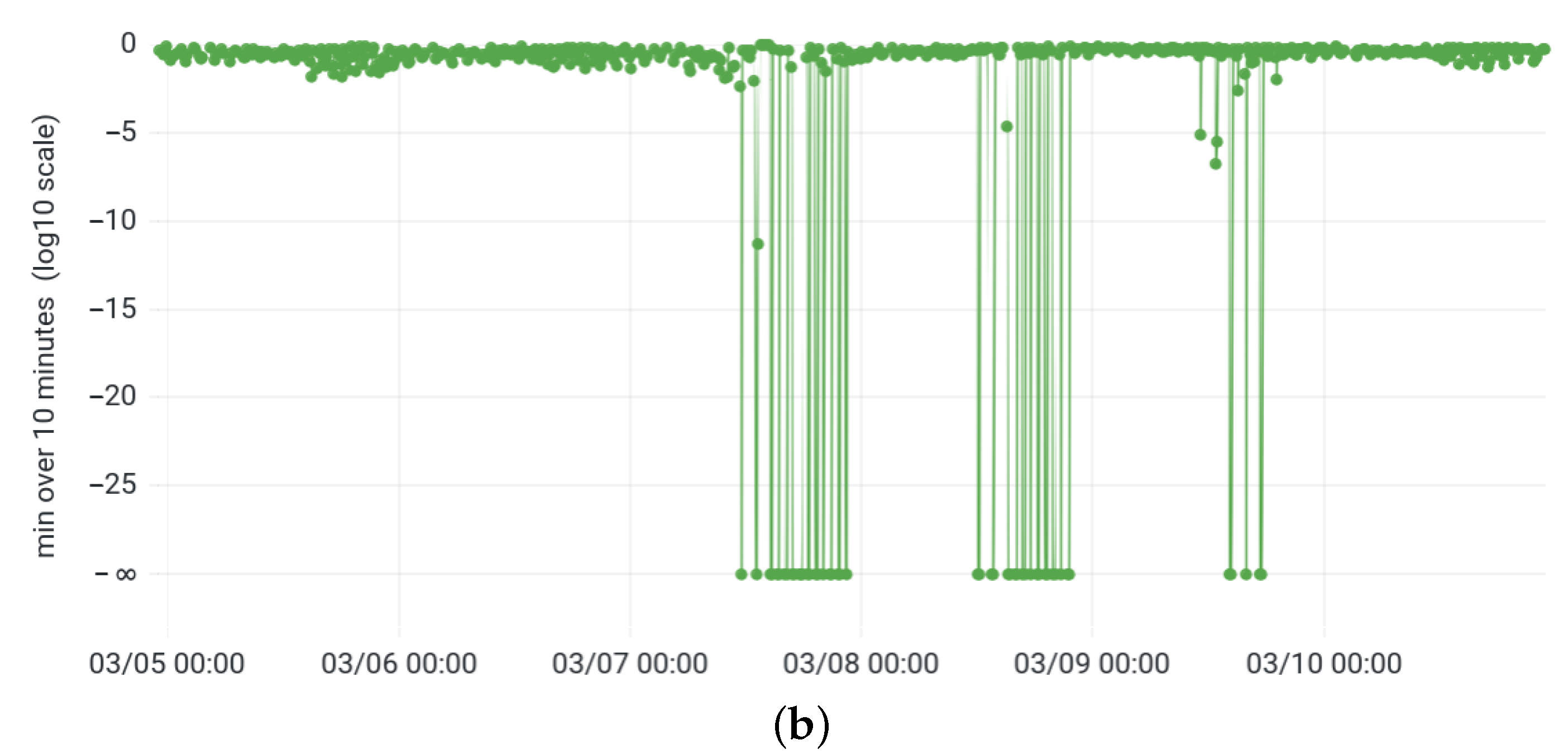
3.1. Background Rejection

Looking at the score time series resulting from the data analysis, many low scores compatible with an SEP event can be found, even when no other experiments confirmed the occurrence of an event. To reduce the background, the same cuts applied on the geomagnetic field intensity, the ISS zenith angle, and the ages of position and flight orientation information for the reference trigger rate definition can be used. Specifically, data collected with a geomagnetic field intensity less than 25,000 nT, a zenith angle greater than 15${}^{\circ }$, an age older than 10 s for the ISS position data, and older than 1 min for the ISS flight orientation, are excluded from SEP events search. Figure 4 shows the effectiveness of those cuts on the score time-series obtained during a confirmed event [13].

In addition to the previous standard cuts, the additional condition $L\ge 1.5R_0$ results in being able to reject an important fraction of noise for the LV1 trigger rate. The effectiveness of this cut is most likely related to the errors introduced by the rate modeling in the low-L bins and is further treated in the Discussion section. Figure 5 compares the LV1 trigger scores obtained by applying only the standard cuts, with those obtained with the additional L cut.

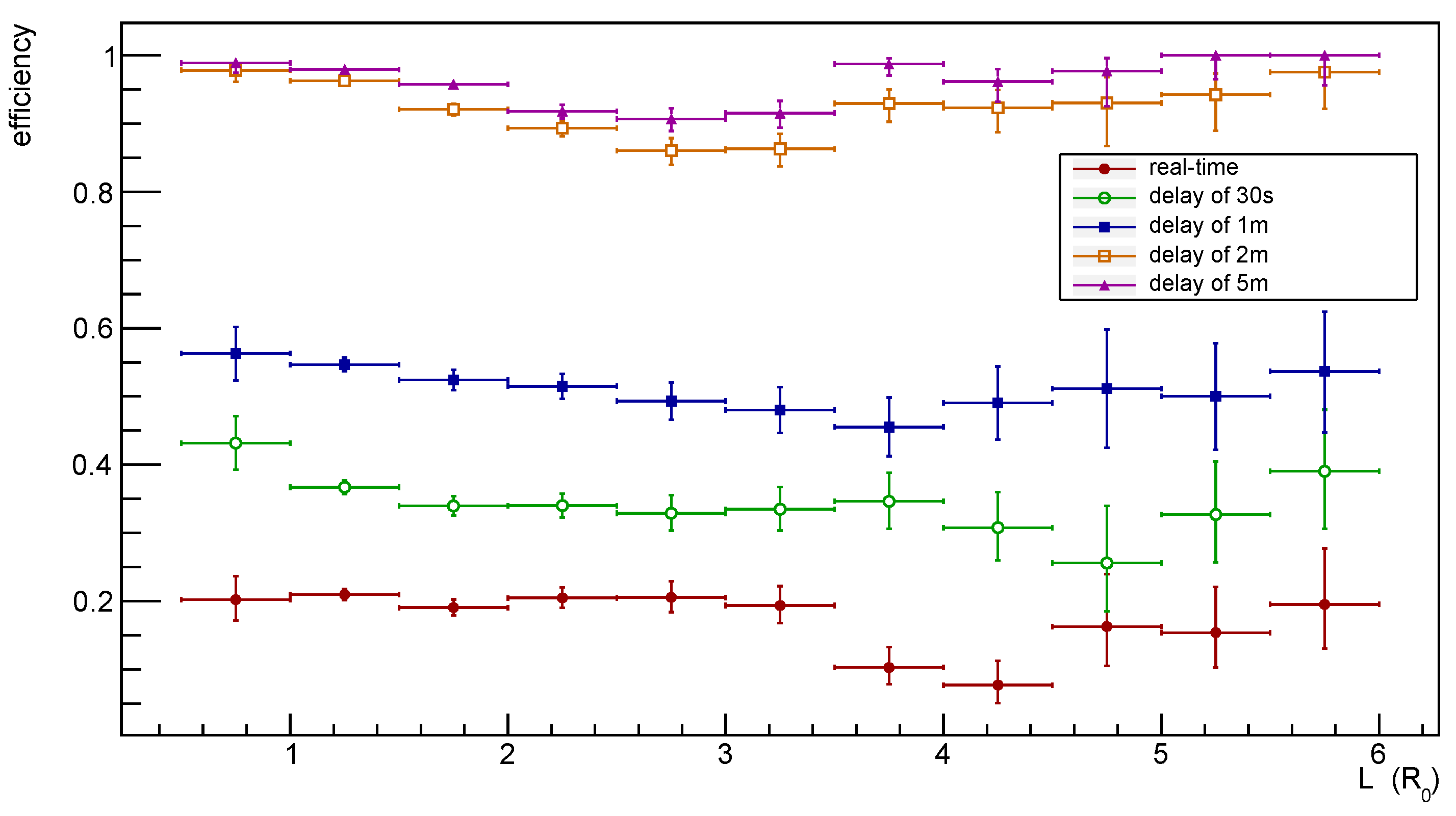
3.2. Efficiency of the Real-Time Monitoring

Due to the delays of the AMI data downlink described in the previous section, the monitoring in real-time can experience some data losses. Figure 6 shows the efficiencies measured for data queries performed with different delays.

4. Discussion

The monitor described in this manuscript uses an architecture similar to the one used for the AMI, foreseeing a later implementation in the AMI itself. However, Figure 6 shows how relying on AMI data negatively affects the real-time monitoring, mining the possibility of launching live alerts for SEP events. This issue could be solved by implementing the analysis directly onboard the ISS. In that case, data would be immediately available and the access to the primary data flow of AMS would also provide access to a broader information. In addition, performing the analysis in space would also give the opportunity to provide an alert system directly on the ISS.

As Figure 3 shows, most of the L bins used for the analysis collect ≳ 100 entries in a 3-day time window, except the bin $[6.0,6.5)R_0$. For $L\ge 6R_0$, ∼10 entries per month of data can be found. The use of a larger time window to collect more statistics would decrease the possibility of performing a real-time analysis efficiently and the use of a larger bin would lower the sensibility in regions where the shielding of the geomagnetic field is minimum. The score values used to highlight SEP events benefits from the use of the information of multiple bins at the same time, therefore the last bin, even if less representative, can still provide a foothold for the weighted averages used in the score calculus.

Another issue in the developed analysis regards the discrepancy between the modeling PDFs used and the actual distributions, which are shown in the Supplementary Materials. Inadequacies in data characterization also introduce some noise that notably affects the LV1 trigger, as indicated by the additional L cut for background rejection. The efficacy of this cut can be understood by examining the detailed trigger rate distributions in the Supplemental Material. Low-L bins exhibit statistics that deviate from Gaussian and Poisson distributions, with a higher prevalence of low rates. A higher proportion of low values results in a generally lower $\mu$, thus leading to a greater frequency of low scores. Triggers other than LV1, as exemplified in Figure 4, are less affected by this problem. In contrast, the LV1 score time-series displays a significant amount of noise when applying only the standard cuts, as seen in Figure 5. Because of these problems, the work presented in this manuscript can be extended by exploring supplemental parameters, beyond L, which could enhance the characterization of the reference distributions.

The background rejection presented here is a fast and preliminary way to lower the possibility of detecting false SEP events. However, the cuts applied by this work are not completely effective and excesses not related to any confirmed SEP event can still be found in the monitor [8].

As Figure 4b and Figure 5b show, SEPs do not cause a single continuous increment in the trigger rates, but rather a series of increments. This is due to the variation of the geomagnetic field intensity during ISS motion. This dynamic could be modeled and a specific algorithm developed to predict the excesses following the initial one and the end of the event itself.

Another feature visible in Figure 4b and Figure 5b is the presence of null scores in the time-series. The occurrence of scores precisely equal to 0 is due to the very high increments SEPs can cause with respect to the nominal rates. Null scores do not affect the possibility of launching SEP alerts and makes choosing a threshold for the alert trigger much easier.

In the end, AMS collects much more information than the one its triggers provide. The instrument detectors can offer additional data about the observed particles, which could improve the SEP identification and the background rejection.

5. Conclusions

The work presented in this manuscript is the first implementation of a real-time monitor for SEP flows near the ISS. Ref. [5] showed how it is possible to detect SEP events using the trigger rates of AMS-02. This monitoring system makes use of that information to allow for the detection of SEP events in real time. However, in order to provide reliable alerts, the delays in the primary data availability need to be reduced and the background rejection has to be improved.

An SEP monitoring system directly onboard AMS on the ISS represents the best solution for a real-time system, avoiding all problems of latency and buffering that are experienced with the on-ground monitoring. Eventually, the use of more information, coming not only from the trigger system but also from all the other AMS detectors, would improve the SEP detection, reducing the number of false positives and improving the efficiency.

References

1. Longair, M. High Energy Astrophysics, 3rd ed.; Cambridge University Press: Cambridge, UK, 2011. [Google Scholar]
2. Raouafi, N.E.; Patsourakos, S.; Pariat, E.; Young, P.R.; Sterling, A.C.; Savcheva, A.; Shimojo, M.; Moreno-Insertis, F.; DeVore, C.R.; Archontis, V.; et al. Solar Coronal Jets: Observations, Theory, and Modeling. Space Sci. Rev. 2016, 201, 1–53. [Google Scholar]
3. Kahler, S.W.; Sheeley, N.R., Jr.; Howard, R.A.; Koomen, M.J.; Michels, D.J.; McGuire, R.V.; Von Rosenvinge, T.T.; Reames, D.V. Associations between coronal mass ejections and solar energetic proton events. J. Geophys. Res. 1984, 89, 9683–9693. [Google Scholar] [CrossRef]
4. AMS-02. Available online: https://ams02.space/ (accessed on 15 October 2023).
5. Faldi, F.; Bertucci, B.; Tomassetti, N.; Vagelli, V. Real-time monitoring of solar energetic particles outside the ISS with the AMS-02 instrument. Rend. Lincei. Sci. Fis. Nat. 2023, 34, 339–345. [Google Scholar] [CrossRef]
6. Hashmani, R.; Konyushikhin, M.; Shan, B.; Cai, X.; Demirköz, M.B. New monitoring interface for the AMS experiment. NIM-A 2023, 1046, 167704. [Google Scholar] [CrossRef]
7. AMI SEP Repository. Available online: https://gitlab.cern.ch/aserpoll/ami-sep (accessed on 15 October 2023).
8. AMI SEP Grafana App. Available online: https://ami-sep-monitor.app.cern.ch (accessed on 15 October 2023).
9. McIlwain, C. Coordinates for mapping the distribution of magnetically trapped particles. J. Geophys. Res. 1961, 66, 3681–3691. [Google Scholar] [CrossRef]
10. Lin, C. Trigger Logic Design Specification, 2005. Internal Document of AMS-02 Collaboration (n. AMS-JT-JLV1-LOGIC-R02c). Available online: https://ams.cern.ch/AMS/DAQsoft/trigger_logic_v02c.pdf (accessed on 15 October 2023).
11. Shea, M.; Smart, D.; Gentile, L. Estimating cosmic ray vertical cutoff rigidities as a function of the McIlwain L-parameter for different epochs of the geomagnetic field. Phys. Earth Planet. Inter. 1987, 48, 200–205. [Google Scholar] [CrossRef]
12. Alken, P.; Thébault, E.; Beggan, C.D.; Amit, H.; Aubert, J.; Baerenzung, J.; Bondar, T.N.; Brown, W.J.; Califf, S.; Chambodut, A.; et al. International Geomagnetic Reference Field: The thirteenth generation. Earth Planets Space 2021, 73, 49. [Google Scholar]
13. Major SEP Events. Available online: https://cdaw.gsfc.nasa.gov/CME_list/sepe/ (accessed on 15 October 2023).
Figure 1. Average live-time of AMS-02 in January 2020 as a function of the L-value of the position of detection. Lower live-times show a higher activity of the instrument, because of a greater flux of particles crossing it. Live-time decreases with increasing L-values, indicating a dependence between the two quantities.
Instruments 07 00038 g001
Figure 2. Map of the L-values calculated on ISS orbit data of January, 2020. The values are expressed in Earth radii units and are averaged in cells 1 (latitude) × 1 (longitude), with an error ≲4%. ISS orbit projection on Earth’s surface spans a latitude range approximately from 52 to + 52 .
Instruments 07 00038 g002
Figure 3. Distribution of the L-values calculated for AMI data of a 3-day period, i.e., 1–3 January 2020. L bins span between 0.5 and 6.5 R 0 and are 0.5 R 0 wide. Every bin collects more than 100 entries, except for the last bin, characterized in general by a much lower statistics (i.e., 10 entries per month).
Instruments 07 00038 g003
Figure 4. Score time-series for the FT rate (corrected by the live-time) in the period 5–11 March 2012, during a confirmed SEP event. (a) Top panel shows the time-series with all the data. (b) Bottom panel shows the same time-series, with the background rejection cuts applied.
Instruments 07 00038 g004
Figure 5. Score time-series for the LV1 trigger rate (corrected by the live-time) in the period March 5–11, 2012, during a confirmed SEP event. (a) Top panel shows the time-series with the standard cuts for background rejection applied. (b) Bottom panel shows the same time-series, with the additional requirement L 1.5 R 0 .
Instruments 07 00038 g005aInstruments 07 00038 g005b
Figure 6. Efficiency of data requests to the AMI database. Efficiencies were measured querying data in real-time and with different delays for 10 days, between 10–20 May 2023. The number of entries obtained after 1 h are used as totals for the efficiencies measurement. Overall, the efficiency increases with the delay and in real-time ϵ 20 % , after 30 s ∼20–30%, after 1 min ∼40–60% and after more than 2 min 80 % .
Instruments 07 00038 g006
Disclaimer/Publisher’s Note: The statements, opinions and data contained in all publications are solely those of the individual author(s) and contributor(s) and not of MDPI and/or the editor(s). MDPI and/or the editor(s) disclaim responsibility for any injury to people or property resulting from any ideas, methods, instructions or products referred to in the content.