DOME: Discrete Oriented Muon Emission in GEANT4 Simulations

Abstract

The simulation of muon tomography requires a multi-directional particle source that traverses a number of horizontal detectors of limited angular acceptance that are used to track cosmic-ray muons. In this study, we describe a simple strategy that can use GEANT4 simulations to produce a hemispherical particle source. We initially generate random points on a spherical surface of practical radius by using a Gaussian distribution for the three components of the Cartesian coordinates, thereby obtaining a generating surface for the initial position of the particles to be tracked. Since we do not require the bottom half of the sphere, we take the absolute value of the vertical coordinate, resulting in a hemisphere. Next, we direct the generated particles into the target body by selectively favoring the momentum direction along the vector constructed between a random point on the hemispherical surface and the origin of the target, thereby minimizing particle loss through source biasing. We also discuss a second scheme where the coordinate transformation is performed between the spherical and Cartesian coordinates, and the above-source biasing procedure is applied to orient the generated muons towards the target. Finally, a recipe based on restrictive planes from our previous study is discussed. We implement our strategies by using G4ParticleGun in the GEANT4 code. While we apply these techniques to simulations for muon tomography via scattering, these source schemes can be applied to similar studies for atmospheric sciences, space engineering, and astrophysics where a 3D particle source is a necessity.

1. Introduction

In the past, a variety of source geometries have been utilized for specific applications in muon imaging simulation studies, including planar surfaces and parabolic beams, as well as hemispherical surfaces [1]. In this study, we describe the implementation of two schemes aimed at building a hemispherical muon source where the generated particles are oriented towards a specific point or plane, using what we call the “selective momentum” direction. While there are different schemes to generate 2D/3D sources, we prefer to use the existing algorithms in GEANT4 [2], i.e., $\mathrm{G}4\mathrm{RandGauss}::\mathrm{shoot}\left(\right)$ and $\mathrm{G}4\mathrm{UniformRand}\left(\right)$ as the distribution function. Whereas the geometrical shape of the 2D/3D sources plays an important role in a particular application, the momentum direction is another variable the user must specify. In this study, we first generate a spherical surface by using three Gaussian distributions for the three components of the Cartesian coordinates and we direct the generated particles from their initial positions on this spherical surface to the preferred location(s) by using a vector constructed, as described in our previous study [3]. This methodology is called discrete oriented muon emission (DOME), where the kinetic energy of the generated particles is intentionally discrete for the computational purposes, as already implemented in another study [4]. In the latter scheme, we generate the initial positions by randomizing the spherical variables, i.e., azimuth and zenith, and we perform the coordinate transformation from the spherical coordinates to the Cartesian coordinates [5,6,7]. We repeat the same operations as performed in the first scheme. This paper is organized as follows. Section 2.1 describes the first scheme that is based on the Gaussian distribution functions, while Section 2.2 consists of the second methodology founded on the coordinate transformation from spherical to Cartesian coordinates. An alternative focusing scheme is explained in Section 3, and we summarize our conclusions in Section 4.

2. Central Focus Scheme

2.1. Generation through Gaussian Distributions

Our objective is to build a hemispherical muon source that surrounds our detector setup [8] similar to the other configurations existing in the literature [9,10,11], as illustrated in Figure 1. First, the particle locations in Cartesian coordinates are generated by using the Gaussian distributions formally defined as G4RandGauss::shoot() in GEANT4 as:

$$x_0=G(\overline{x},{\sigma }_x,x)=\mathrm{G}4\mathrm{RandGauss}::\mathrm{shoot}\left(\right),$$

(1)

and

$$y_0=G(\overline{y},{\sigma }_y,y)=\mathrm{G}4\mathrm{RandGauss}::\mathrm{shoot}\left(\right),$$

(2)

and

$$z_0=G(\overline{z},{\sigma }_z,z)=\mathrm{G}4\mathrm{RandGauss}::\mathrm{shoot}\left(\right).$$

(3)

where $\overline{x}=\overline{y}=\overline{z}=0$ and ${\sigma }_x={\sigma }_y={\sigma }_z=1$ by definition. The generated spatial points are renormalized in order to form a unit sphere, as indicated in

$$x_0^{*}=\frac{x_0}{\sqrt{x_0^2+y_0^2+z_0^2}},y_0^{*}=\frac{y_0}{\sqrt{x_0^2+y_0^2+z_0^2}},z_0^{*}=\frac{z_0}{\sqrt{x_0^2+y_0^2+z_0^2}}.$$

(4)

Given a sphere of radius denoted by R, the initial positions on the spherical surface of radius R in cm in the Cartesian coordinates are obtained as follows

$$x_i=R\ast x_0^{*},y_i=R\ast \left|y_0^{*}\right|=R\ast \mathrm{ABS}\left(y_0^{*}\right),z_i=R\ast z_0^{*}.$$

(5)

where the y-component of the Cartesian coordinates constituting the vertical axis is positively defined in order to yield the hemispherical surface. Then, the generated particles on the spherical surface are directed to the origin

$$x_f=0,y_f=0,z_f=0.$$

(6)

By constructing a vector from the hemispherical surface to the origin, one obtains

$$px=x_f-x_i,py=y_f-y_i,pz=z_f-z_i.$$

(7)

Thus, the selective momentum direction denoted by $\overrightarrow{P}=(P_x,P_y,P_z)$ is

$$P_x=\frac{px}{\sqrt{p{x}^2+p{y}^2+p{z}^2}},P_y=\frac{py}{\sqrt{p{x}^2+p{y}^2+p{z}^2}},P_z=\frac{pz}{\sqrt{p{x}^2+p{y}^2+p{z}^2}}.$$

(8)

The developed code via the Gaussian distributions is given in Appendix A.

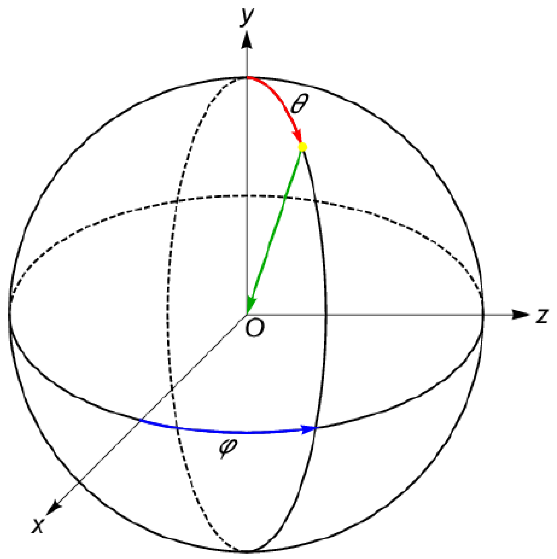
2.2. Generation via Coordinate Transformation

The second scheme is composed of the coordinate transformation, as depicted in Figure 2. To begin, two numbers, $q_1$ and $q_2$, are uniformly generated and inserted into the associated expression of the spherical variables as follows

$$q_1=\mathrm{G}4\mathrm{UniformRand}\left(\right),$$

(9)

and

$$q_2=\mathrm{G}4\mathrm{UniformRand}\left(\right).$$

(10)

The surface generation is initiated by randomizing $\theta$ as well as $\phi$, as shown in

$$\theta =arccos(2\times q_1-1),$$

(11)

and

$$\phi =2\times \pi \times q_2.$$

(12)

The coordinate transformation yields the generated points on the hemispherical surface of radius R in Cartesian coordinates, as described in

$$x_i=R\sin \theta \cos \phi$$

(13)

$$y_i=R\cos \theta =R\left|\cos \theta \right|=R ABS\left(\cos \theta \right)$$

(14)

$$z_i=R\sin \theta \sin \phi$$

(15)

The y-component of the Cartesian coordinates constituting the vertical axis is positively defined in order to yield the hemispherical surface as usual. Then, the generated particles on the spherical surface are again directed to the origin

$$x_f=0,y_f=0,z_f=0.$$

(16)

By constructing a vector from the hemispherical surface to the origin, one obtains

$$px=x_f-x_i,py=y_f-y_i,pz=z_f-z_i.$$

(17)

Thus, the selective momentum direction denoted by $\overrightarrow{P}=(P_x,P_y,P_z)$ is

$$P_x=\frac{px}{\sqrt{p{x}^2+p{y}^2+p{z}^2}},P_y=\frac{py}{\sqrt{p{x}^2+p{y}^2+p{z}^2}},P_z=\frac{pz}{\sqrt{p{x}^2+p{y}^2+p{z}^2}}.$$

(18)

The obtained code by means the coordinate transformation is shown in Appendix B. A simulation preview through either scheme is displayed in Figure 3.

3. Restrictive Planar Focus Scheme

As described in another study [3], the generated particles from any initial point on the hemispherical surface can be directed to a location randomly selected on a pseudo plane that restricts the momentum direction and which also leads to the minimization of the particle loss. Thus, the particle locations in cm on a restrictive plane of $2L\times 2D$${\mathrm{cm}}^2$ situated at y = 0 will have the spatial coordinates, such that

$$x_f=-L+2\times L\times \mathrm{G}4\mathrm{UniformRand}\left(\right),y_f=0,z_f=-D+2\times D\times \mathrm{G}4\mathrm{UniformRand}\left(\right).$$

(19)

Then, by constructing a vector from the generated hemispherical surface to the restrictive plane, one obtains

$$px=x_f-x_i,py=y_f-y_i,pz=z_f-z_i.$$

(20)

Thus, the selective momentum direction, i.e., $\overrightarrow{P}=(P_x,P_y,P_z)$, is

$$P_x=\frac{px}{\sqrt{p{x}^2+p{y}^2+p{z}^2}},P_y=\frac{py}{\sqrt{p{x}^2+p{y}^2+p{z}^2}},P_z=\frac{pz}{\sqrt{p{x}^2+p{y}^2+p{z}^2}}.$$

(21)

4. Conclusions

In this study, we explored the use of random number generators that are defined in the GEANT4 code. This can provide a number of source schemes where the first strategy is based on the Gaussian distributions, whereas the latter procedure requires a coordinate transformation to spherical variables. Finally, we obtain a hemispherical muon source where the kinetic energies of the generated muons are binned, and the momentum directions of these generated muons are selected by means of vector constructions. We call this source discrete oriented muon emission (DOME). DOME has been developed for simulations of muon tomography scenarios where the volume of interest is contained in a gap between detection layers, and the hemispheric source surrounds the entire setup. However, it can find applications in a broader array of use cases. For example, as demonstrated in [1], hemispheric sources are computationally efficient and at the same time unbiased for measurements of the cosmic muon flux where the detector has a complex geometry. Moreover, nothing prevents applications of the same method in simulations of muon radiography setups for volcanoes or pyramids or other very large objects of interest that are distant from the detector [12] where solid angle restrictions can optionally be imposed to increase computational efficiency.

References

1. Pagano, D.; Bonomi, G.; Donzella, A.; Zenoni, A.; Zumerle, G.; Zurlo, N. EcoMug: An Efficient COsmic MUon Generator for cosmic-ray muon applications. Nucl. Instrum. Methods Phys. Res. Sect. A Accel. Spectrom. Detect. Assoc. Equip. 2021, 1014, 165732. [Google Scholar] [CrossRef]
2. Agostinelli, S.; Allison, J.; Amako, K.; Apostolakis, J.; Araujo, H.; Arce, P.; Asai, M.; Axen, D.; Banerjee, S.; Barrand, G.; et al. GEANT4—A simulation toolkit. Nucl. Instrum. Methods Phys. Res. Sect. A Accel. Spectrom. Detect. Assoc. Equip. 2003, 506, 250–303. [Google Scholar] [CrossRef]
3. Topuz, A.I.; Kiisk, M.; Giammanco, A. Particle generation trough restrictive planes in GEANT4 simulations for potential applications of cosmic ray muon tomography. arXiv 2022, arXiv:2201.07068. [Google Scholar]
4. Topuz, A.I.; Kiisk, M. Towards energy discretization for muon scattering tomography in GEANT4 simulations: A discrete probabilistic approach. arXiv 2022, arXiv:2201.08804. [Google Scholar]
5. Marsaglia, G. Choosing a point from the surface of a sphere. Ann. Math. Stat. 1972, 43, 645–646. [Google Scholar] [CrossRef]
6. Tashiro, Y. On methods for generating uniform random points on the surface of a sphere. Ann. Inst. Stat. Math. 1977, 29, 295–300. [Google Scholar] [CrossRef]
7. Weisstein, E.W. “Disk Point Picking”. From MathWorld-A Wolfram Web Resource. 2011. Available online: http://mathworld.wolfram.com/ (accessed on 22 May 2022).
8. Georgadze, A.; Kiisk, M.; Mart, M.; Avots, E.; Anbarjafari, G. Method and Apparatus for Detection and/or Identification of Materials and of Articles Using Charged Particles. US Patent 16/977,293, 7 January 2021. [Google Scholar]
9. Borozdin, K.N.; Hogan, G.E.; Morris, C.; Priedhorsky, W.C.; Saunders, A.; Schultz, L.J.; Teasdale, M.E. Radiographic imaging with cosmic-ray muons. Nature 2003, 422, 277. [Google Scholar] [CrossRef] [PubMed]
10. Frazão, L.; Velthuis, J.; Maddrell-Mander, S.; Thomay, C. High-resolution imaging of nuclear waste containers with muon scattering tomography. J. Instrum. 2019, 14, P08005. [Google Scholar] [CrossRef]
11. Frazão, L.; Velthuis, J.; Thomay, C.; Steer, C. Discrimination of high-Z materials in concrete-filled containers using muon scattering tomography. J. Instrum. 2016, 11, P07020. [Google Scholar] [CrossRef]
12. Bonechi, L.; D’Alessandro, R.; Giammanco, A. Atmospheric muons as an imaging tool. Rev. Phys. 2020, 5, 100038. [Google Scholar] [CrossRef]
Figure 1. Delineation of the generated particles from the hemispherical source with a momentum direction towards the origin.
Instruments 06 00042 g001
Figure 2. Spherical variables consisting of θ and φ with respect to the Cartesian coordinates (x,y,z).
Instruments 06 00042 g002
Figure 3. Hemispherical muon source in GEANT4.
Instruments 06 00042 g003
Publisher’s Note: MDPI stays neutral with regard to jurisdictional claims in published maps and institutional affiliations.