Article

Machine Learning of Nonequilibrium Phase Transition in an Ising Model on Square Lattice

by
Dagne Wordofa Tola
1,2,* and
Mulugeta Bekele
1,*
1
Department of Physics, Addis Ababa University, Addis Ababa P.O.Box 1176, Ethiopia
2
Department of Physics, Dire Dawa University, Dire Dawa P.O. Box 1362, Ethiopia
*
Authors to whom correspondence should be addressed.
Condens. Matter 2023, 8(3), 83; https://doi.org/10.3390/condmat8030083
Submission received: 8 August 2023 / Revised: 30 August 2023 / Accepted: 1 September 2023 / Published: 15 September 2023

Abstract

:
This paper presents the investigation of convolutional neural network (CNN) prediction successfully recognizing the temperature of the nonequilibrium phase transitions in two-dimensional (2D) Ising spins on a square lattice. The model uses image snapshots of ferromagnetic 2D spin configurations as an input shape to provide the average output predictions. By considering supervised machine learning techniques, we perform Metropolis Monte Carlo (MC) simulations to generate the configurations. In the equilibrium Ising model, the Metropolis algorithm respects detailed balance condition (DBC), while its nonequilibrium version violates DBC. Violating the DBC of the algorithm is characterized by a parameter 8 < ε < 8 . We find the exact result of the transition temperature T c ( ε ) in terms of ε . If we set ε = 0 , the usual single spin-flip algorithm can be restored, and the equilibrium configurations generated with such a set up are used to train our model. For ε 0 , the system attains the nonequilibrium steady states (NESS), and the modified algorithm generates NESS configurations (test dataset). The trained model is successfully tested on the test dataset. Our result shows that CNN can determine T c ( ε 0 ) for various ε values, consistent with the exact result.

1. Introduction

The world around us manifests itself in various forms: living and non-living matter. On the other hand, there are many phases of matter, and one can consider transitions between these phases. In physics, phase transitions (PTs) refer to changes in the collective behavior of a system as it undergoes a transition from one phase to another. The concept of universality classes is commonly found in various fields of physics, from condensed matter physics to complex systems. Universality classes are used to categorize different physical phenomena based on their similarities in behavior near PTs or near critical points. Currently, the standard theory and general framework for the critical phenomenon near continuous PTs is well understood in equilibrium systems [1,2,3]. The modeling and simulation of the physical phenomena of interest can succeed either from analytical or numerical methods [4]. However, the study of PTs between nonequilibrium statistical states has consistently been among the main subjects of ongoing research and exploration [5,6,7,8,9,10,11,12]. Nonequilibrium PTs are transitions that occur in systems that are not at the thermodynamic equilibrium. Before delving into our circumstantial system model, some examples of different types of nonequilibrium PTs are briefly provided as follows.
  • Directed percolation transition: Directed percolation is a type of PT that occurs in systems with a preferred direction of propagation. It is commonly used to model phenomena, such as spreading of epidemics, forest fires, or chemical reactions. The PT is characterized by the sudden emergence of a spanning cluster that spreads through the system.
  • Active matter transitions: Active matter refers to systems composed of self-propelled particles that can extract energy from the environment to exhibit collective behaviors. Examples include dense suspensions of swimming bacteria or assemblies of self-propelled robots. Active matter can undergo PTs, such as the transition between a disordered and a collectively ordered state, often accompanied by dynamic pattern formations.
  • Self-organized criticality: Self-organized criticality is a concept that describes how complex systems naturally evolve to a critical state. In these systems, small local perturbations can trigger cascades of events, leading to large-scale avalanches or fluctuations. Examples include sand pile models, earthquakes, or forest fires. These transitions are characterized by power law distributions of event sizes and long-range correlations.
  • Berezinskii–Kosterlitz–Thouless transition: This transition occurs in 2D systems, such as thin films or superconducting materials, where the conventional long-range order is disrupted due to the presence of topological defects called vortices.
These are just a few examples of nonequilibrium PTs. Each type has its own characteristic features and mathematical formulations. Understanding these transitions is essential for studying a wide range of complex systems across multiple disciplines. Nonequilibrium situations are far less completely understood, although classes have of course been studied over the decades. This is an important area of research since much of its functional nature resides out of equilibrium-including quantum annealing uses for some current quantum computers for which the Ising model is directly relevant. A deeper understanding of relaxation (in dissipative systems) or thermal equilibration, more generally, is extremely desirable.
Identifying the critical points of various phases within the parameter space is a fundamental undertaking in the fields of statistical mechanics and condensed matter physics. Machine learning (ML) is the field of study concerned with algorithms that are designed to improve their performance by obtaining experience from data [13]. Relatively recently, the utilization of these techniques was successfully employed in various domains, such as investigating the phases of the Ising model [14,15,16,17], PT in the Bose–Hubbard [18,19], disordered quantum systems [20,21], and material properties [22]. In this paper, we introduce the application of ML to nonequilibrium PT, which can be accomplished based on the well-established features of modern theories of PT in equilibrium systems. In equilibrium systems, PT is generically described by singularities in the free energy and its derivatives. Such singularity causes a discontinuous property of thermodynamic quantities near the transition point. Phenomenologically, the PT is defined regarding an order parameter, which has a nonzero value in the ordered phase while it vanishes in the disordered phase [23,24,25]. Within the scope of this paper, the paradigmatic example that we will be working on is a two-dimensional (2D) Ising spin system on a square lattice. It is interesting to note that the 2D Ising spin on a square lattice is simple such that it can be exactly solved [23]. Even though it is exactly solvable, it is still a topic of ongoing research that is frequently used in the context of ML [14,15,16,17,26,27,28,29,30,31,32,33]. In this investigation, first we try to perform the graphical solution (7) of the nonequilibrium transition temperature; see Appendix A.1. Then, we look at the possibility of a nonequilibrium phase transition occurring within the Ising model that breaks the principle of detailed balance through machine learning. To be more explicit, we aim to find the nonequilibrium phases and the transition temperatures by applying convolutional neural networks (CNNs) based on the general framework of supervised learning discussed in [34]. This framework was reviewed before in Statistical Mechanics of Deep Learning, which also briefly explains the connection between deep learning and the modern subject of statistical physics.
According to the findings presented in Ref. [29], the application of ML to the issue of phases of matter has, for the most part, been effective. Motivated by this work, we aim to extend this ML application to the case of the nonequilibrium phase transition. For its compatibility to our present study, the Ising model which was addressed in [35] becomes the primary focus of our attention. We employ the Monte Carlo (MC) approach [36,37,38,39] to generate a properly distributed dataset of Ising spin configurations on the L × L square lattice (where L is its linear size), together with their associated labels, while considering supervised learning techniques. Accordingly, by the context of equilibrium and nonequilibrium systems, we are referring to two different spin update rules: (i) the rule that holds the DBC and (ii) the rule that breaks the DBC, respectively. The former is used to generate the train dataset, while the latter is used to generate the test dataset, which can be seen from some representative configurations illustrated in Appendix A.2 (Figure A3).
We build a CNN using open-source software [40]; see Appendix A.2 and an example shown in Figure A4 for more details. We train our model on the training dataset, and it is effectively validated to classify the simulation results of the equilibrium 2D Ising model into the ferromagnetic (FM) or “ordered state” and the paramagnetic (PM) or “disordered state” phases. The classification of these results was also successfully validated; see, for example, [29,30]. The main goal of this work is to evaluate the generalization reach of the CNN by testing it with configurations (test dataset) from a system that is not in equilibrium. Intriguingly, in addition to accurately categorizing the configurations, we demonstrate that the CNN can exhibit the critical temperature of the nonequilibrium PT. Our finding is very close to the exact solution (7), and also consistent with the MC results provided in Ref. [35].
The remaining sections are organized as follows: In Section 2, we present the model considered in this research, followed by a concise description of the Metropolis MC method for generating image samples of Ising configurations. Some of the results of this study are then illustrated in Section 3. Finally, we provide a summary of the main results and discussion as presented in Section 4.

2. Description of the Model and Metropolis Monte Carlo Method

We consider the 2D Ising model on a square lattice of linear size L sites. The system size ( N = L × L ) is equal to the total number of spins (N), which means that each of the sites contains one spin that points either up or down ( ± 1 ). If we assume zero magnetic fields, the nearest-neighbor interaction energy of the (ferromagnetic) Ising model is given as
E = J i , j σ i σ j ,
where σ i = ± 1 denotes the value of the spin at site i = { 1 , , N } , the indices i , j represent the nearest-neighbor pairs [36,37], and a ferromagnetic energy scale J > 0 refers to the strength of the exchange interaction. At the critical (or transition) temperature, the system exhibits a second-order phase transition. The transition temperature of the nearest-neighbor equilibrium Ising model, for an infinite square lattice, was derived [23] to be 2 / ln ( 1 + 2 ) ; see Equation (6). In this case, the system is assumed to be a magnetized state when its temperature is lower than 2 / ln ( 1 + 2 ) , which is known as the ordered state (FM phase). On the other hand, the system is said to be in the disordered state (PM phase) if its temperature is higher than 2 / ln ( 1 + 2 ) . The magnetization per spin is what determines the value of the order parameter
m = 1 N i N σ i .
This quantity (2) distinguishes the two phases that are realized by the system. It is zero (nonzero) in the disordered (ordered) phase.

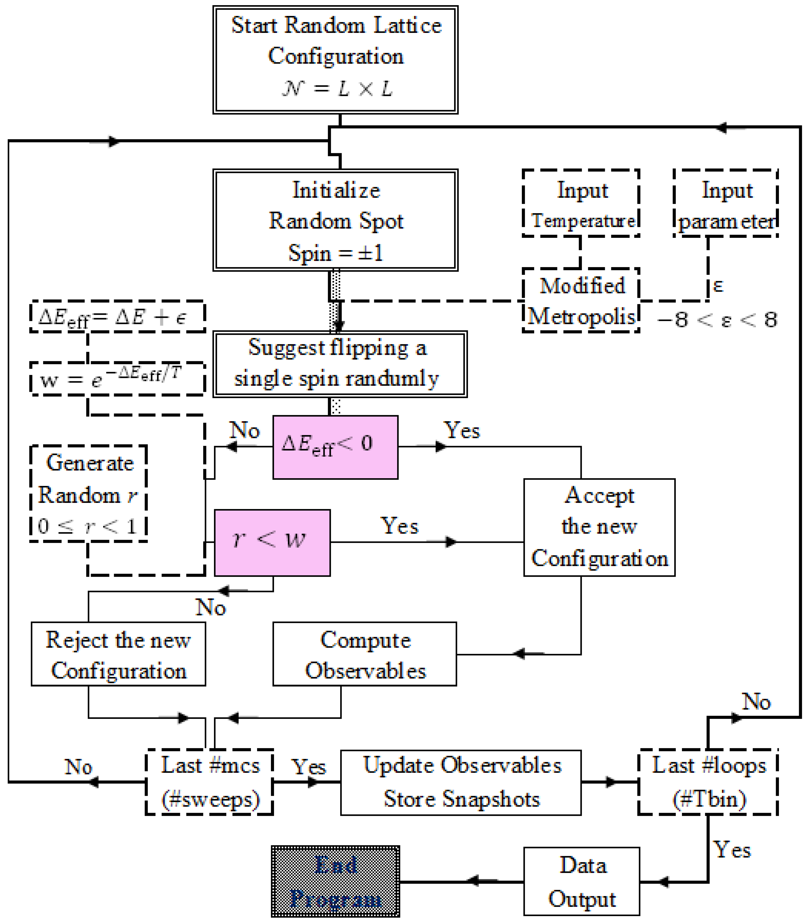
2.1. The Modified Metropolis Algorithm

Let us consider a system that is in contact with a heat bath and produces stochastic spin flips, following Ref. [41]. In the context of the equilibrium Ising model, it can be observed that the system attains thermal equilibrium over a significant time and thus the steady-state distribution can be accurately described by the Boltzmann distribution. This is a valuable approach for establishing transition rates and calculating the probabilities of spin flipping. The Metropolis algorithm [38] is the transition rate that is commonly used and can be stated as
W = MIN 1 , e Δ E / k B T ,
where W represents the rate of change from state b (before flip) to another state a (after flip), Δ E = E a E b is the change in energy that occurs as a result of this transition, and k B denotes the known Boltzmann’s constant. In this context, the unit of temperature T is linked to the units of J / k B . (For the remainder of this description, we will assume k B = 1 , and thus, T = T / J becomes dimensionless.) The defined algorithm (3) meets the requirements of DBC. The aforementioned statement denotes that there exists a microscopic reversibility of every elementary process, which is counterbalanced by its corresponding reverse process [42]. That is, W b a p eq b = W a b p eq a , where p eq b exp [ E b / T ] . Therefore, the ratio w = W b a / W a b gives w = exp [ Δ E / T ] .
The topic of nonequilibrium phase transitions is examined with emphasis on fundamental characteristics, such as the role of DBC violation in generating effective (long-range) interactions [34]. The equilibration process is not solely dependent on the presence of DBC, as it serves as a sufficient but not a necessary condition. The objective of this study is to deliberately violate the DBC to induce a state of fluctuation in the system. As noted in reference [35], there exists a scenario in which the system undergoes an order–disorder phase transition that is different from the typical transitions of the equilibrium case. If ε 0 denotes the parameter violating the DBC, it is possible to substitute Δ E in Equation (3) with
Δ E eff = Δ E + ε ,
and the ratio becomes w = e ( Δ E + ε ) / T . It can be inferred that when ε is positive, Δ E eff is greater than Δ E , whereas when ε is negative, Δ E eff is less than Δ E . The former does not facilitate the process of spin flipping, whereas the latter significantly promotes the likelihood of spin flipping. In contrast to spins subjected to the conventional Metropolis algorithm (3), spins subjected to the modified flipping rates effectively undergo distinct (transition) temperatures. When ε < 0 ( ε > 0 ), it is reasonable to assume that the spins are coupled to a reservoir at a higher (lower) effective temperature ( T eff ). It should be noted that T eff is not uniform across all spins in the system; see Appendix A.1. Thus, “the system is out-of-equilibrium, and a transition is a nonequilibrium phase transition. The property of this transition would be a characteristic of the nonequilibrium steady state (NESS) exhibited by the system” [35]. It can be inferred that, unlike an equilibrium system, the distribution of microstates in the NESS cannot be characterized by the Boltzmann distribution. The transition rate for flipping a spin σ i b σ i a can be determined using this definition (4),
W ( ± σ i σ i ) = e ( ε ± Δ E ) / T , if ε ± Δ E > 0 ; 1 , otherwise .
Here Δ E = 2 J σ i j σ i j { 8 , 4 , 0 , 8 , 4 } [ J ] where σ i j refers to j = { left , right , top , bottom } nearest neighbors of the i th  site, and the symbol ‘≡’ refers to an alternative approach for Ising on a square lattice that involves Δ E , which can assume discrete values from { 8 , 4 , 0 , 4 , 8 } using the units of J. The algorithm given in Equation (5) still respects the DBC when | ε | 8  [43]. However, Equation (5) violates the DBC for 8 < ε < 8 (with ε 0 ) since it is impractical to obtain a unique T eff value for which the transition probabilities for all feasible Δ E values obey the DBC. According to the established notation, the nonequilibrium phase transitions may occur within the system, and the transition temperature T c must fulfill the relation
T c = 0 < T c < T c 0 if 8 < ε < 0 ; T c 0 < T c < 2 T c 0 if 0 < ε < 8 ,
where T c 0 is the transition temperature of the equilibrium ( ε = 0 ) case. We are essentially interested in some ε values of 8 < ε < 8 as shown in Figure 1. Referring to a systematic graphical solution presented in (Appendix A.1), the exact result follows that
T c exact ( ε ) T c = ( 0.5 + ε / 16 ) T c 0 , for 8 < ε < 4 ; ( 1 + 3 ε / 16 ) T c 0 , » 4 ε 4 ; ( 1.5 + ε / 16 ) T c 0 , » 4 < ε < 8 ,
where T c 0 T c ( ε = 0 ) = 2 / ln ( 1 + 2 ) .
Figure 1 shows the transition temperature T c versus parameter ε as plotted using this Equation (7). More specifically, consider two ε values ( ε = ± 2 ); conveniently, we get that T c exact ( ε = ± 2 ) 3.1201 ( 1.4182 ). Remarkably, we see that our numerical result (see Figure 3 and Table 1) is very close to this result.
Figure 1. Transition temperature T c as a function of parameter ε . A plot of Equation (7). The horizontal dashed line represents T c ( ε = 0 ) = T c 0 , where T c 0 = 2 / ln ( 1 + 2 ) . The dotted horizontal lines are T c ( ε = 8 ) = 0 × T c 0 (lower) and T c ( ε = + 8 ) = 2 × T c 0 (upper).
Condensedmatter 08 00083 g001

2.2. Generating 2D Images of Ising Spin Configurations
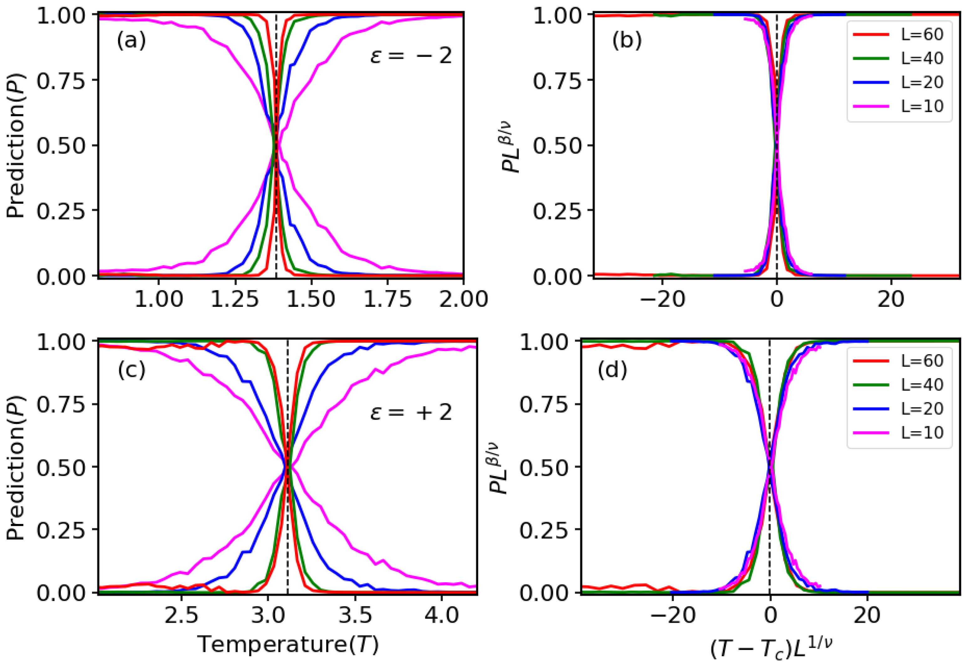
Making use of the modified Metropolis rule (5), we achieve Monte Carlo (MC) simulations of the Ising model; see the flow chart shown in Appendix A.2 (Figure A2). The simulations are performed on a square lattice ( Lx = Ly ) of system size N = L 2 , inducing the periodic boundary condition in both (x and y) directions. For each system, we start the simulations from an initial, high temperature (with random spin initial configurations) and perform standard MC sweeps (MCS) for generating the required samples of L × L Ising spin configurations as data for the supervised ML approach  [36,37,38,39]. Examples of configurations are shown in Figure A3. For all datasets used in Section 3, the simulation is performed with three ε = { 0 , 2 , 2 } values. First, we set ε = 0 and generate the configurations for the training dataset. This comprises about 80% of the total data (where 10% is again reserved for validation). Next, we set ε = 2 to generate the test dataset, which incorporates the remaining 20% of the total data, and the procedure is the same for ε = 2 . We restart and repeat this procedure for all system sizes. Furthermore, one can save the trained sequential model using TenserFlow s   Keras   API , and later it can be loaded to test the configurations from different discrete ε values. Efficiently, this can be used to study the qualitative dependence of T c on the parameter ε ; see an example presented in Appendix A.3 (Figure A5).

3. Results

In the current section (Section 3), we briefly present the main numerical results obtained using a neural network model (CNN). Similar to the previous works (literature), we train the model on equilibrium Ising spin configuration. After training on an adequately large sample size at temperatures T > T c 0 and T < T c 0 , the CNN can correctly classify configurations in a valid dataset as illustrated in Figure 2a for configurations with the given linear size, L = { 10 , 20 , 40 , 60 } . Systematically, finite-size scaling (FSS) is capable of narrowing in on the thermodynamic result of T c 0 in a manner comparable to that of magnetization [29], Figure 2b displays that a data collapse yields a critical exponents estimate of ν 1.00 ± 0.01 and β 0.125 ± 0.002 , while a size scaling of the crossing temperature yields an estimate of T c 0 2.2687 (see Appendix A.4).
More interestingly, “the generalization competency of the neural networks lies in their ability to provide correct predictions further than the datasets with which they were trained”. Accordingly, the trained CNN is provided with a test dataset of configurations from a 2D Ising model in which data generation was incorporated by changing the update rules where the violation of the DBC is accountable. This is intended to answer the question “Does CNN that trained on equilibrium phase transition in Ising model with detailed balance able to recognise the nonequilibrium phase transition?”. Thus, next, we present the results of this scenario by using our CNN, which is already trained and validated on configurations for the square-lattice ferromagnetic Ising model, and provide it with a test dataset generated by modified Metropolis MC simulations for the same sizes as L in Figure 2. In Figure 3, we illustrate the average of prediction P versus temperature T for configurations from two different test datasets ( ε = ± 2 ) of each with four linear sizes (see keys). The dashed lines denote the estimated values of the transition temperatures (a) T c 1.377 , and (c) T c 3.107 . Clearly we see that T c ML ( ε = ± 2 ) is close to T c exact ( ε = ± 2 ) obtained in Equation (7). On the right panel, ‘b’ and ‘d’ represent the corresponding data collapse P L β / ν versus ( T T c ) L 1 / ν allowing us to successfully compute the critical exponents, ν 1.02 ± 0.02 and β 0.126 ± 0.003 . Our results are consistent with the MC result reported in [35].

4. Summary and Conclusions

In this study, a supervised machine learning (ML) surrogate approach is applied based on convolutional neural networks (CNNs) to predict the nonequilibrium transition temperature from paramagnetic (PM) to ferromagnetic (FM) state, in 2D Ising model on a square lattice. This work relies on the previous study [35] in which a modified Metropolis algorithm, and a modified Glauber algorithm were proposed to prospect the nature of nonequilibrium phase transition (PT) in the same 2D Ising model, including the order of the PT, as well as its universality class. More specifically, nonequilibrium PT, where the detailed balance condition (DBC) is not fulfilled and the system reaches a nonequilibrium steady state (NESS) which is not described by Boltzmann statistics, were addressed by the modified Metropolis algorithms. For this study, with this in mind, we intended to implement supervised ML. In literature, different architectures of neural networks were implemented to predict the equilibrium transition temperature from PM phase to FM phase, for example, by training on a square lattice and testing the trained model on triangular lattice. There, it was provided that CNN succeeded in accurately predicting the transition temperature as well as recovering the correct finite-size scaling (FSS) law for the transition temperature. Therefore, the main goal of the present study is to extend this method to nonequilibrium PT in the specific case where the DBC is not fulfilled.
Accordingly, we trained a CNN on a sample of representative Ising spin configurations at various temperatures generated by Monte Carlo (MC) simulations equipped with the usual Metropolis algorithm, in the case of equilibrium PT, where the spin’s update rule is compliant with the DBC. Then, the trained CNN is tested on a set of nonequilibrium configurations generated by MC simulations equipped with the modified Metropolis algorithm. That is, the modified update rule violates the DBC. In the model, violating DBC is designated by a parameter ε that is fixed to take values in the range 8 < ε < 8 ). We have derived the exact solution of the nonequilibrium transition temperature T c ( ε ) , Equation (7). This solution suggests that only the parameter ε affects the transition temperature. For ε = 0 , the equilibrium transition T c 0 can be retrieved. For ε 0 , the system reaches the NESS; this state cannot be characterized using the Boltzmann distribution, and the numerical results are consistent with the exact solution. For instance, for ε = { 2 , 2 } , the averaged output layer prediction is (i) T c ( ε = 2 ) 1.3769 , and (ii) T c ( ε = + 2 ) 3.1071 . These results of T c ( ε ) are close to the values of T c 1.4182 ( T c 3.1201 ), obtained with Equation (7). The discrepancy is mainly related to the role of Δ E = 0 in the modified update rule when we generate the configurations, while it is reasonably neglected in our calculation; see Equation (A4) and Appendix A.3.
In Table 1, we provided a summary of the values of T c ( ε ) that were obtained using the modified Metropolis method using MC simulations (literature) and the supervised ML method (our study). As summarized in this table, we see that MC and ML results are almost in agreement with each other.
Table 1. A summary of the values of transition temperature T c ( ε ) for ε = ± 2 computed via supervised ML compared with exact result as well as the MC result reported in [35]. In our study, the equilibrium transition T c ( ε = 0 ) is used for validation. The error estimates are given in parentheses.
Parameter T c ( ε ) ExactMachine LearningMonte Carlo
ε (This Work) Equation (7) T c ML (This Work) T c MC Ref. [35]
0 2 / ln ( 1 + 2 ) 2.2692 2.2687 ( 15 )
−2 5 / 4 ln ( 1 + 2 ) 1.4182 1.3769 ( 87 ) 1.3604 ( 3 )
+2 11 / 4 ln ( 1 + 2 ) 3.1201 3.1071 ( 175 ) 3.1267 ( 4 )
In conclusion, it is found that the prediction of the CNN trained on equilibrium configurations, where it is tested on nonequilibrium configurations, provides similar transition temperature and FSS to the modified Metropolis algorithm, thereby demonstrating the capacity of this class of surrogate models to extend to configurations far from the configurations used in the training stage. Investigating how these methods can be extended to different spin models and other types of nonequilibrium PT is one of the fascinating questions that might be asked in this area. For example, one can investigate whether or not this numerical method can be extended to the nonequilibrium PT in an active spherical model. The spherical model is another model that can be exactly solved. In practice, it is used to characterize a wide variety of critical phenomena, including the ferromagnetic transition and the Bose–Einstein condensation, for example. In this particular piece of work, we focused solely on the model’s static characteristics. It has come to the attention of the authors that the parameter ε has been included here to only play the role of violating the DBC. In a remarkable turn of works, the subsequent focus of our research will be on the mathematical formalization as well as its complete physical description. Therefore, investigating the dynamical features of the models that violate DBC signifies a more intriguing potential course of the future direction.

Author Contributions

Conceptualization, D.W.T. and M.B.; Methodology, D.W.T. and M.B. Validation, D.W.T.; Formal analysis, D.W.T.; Investigation, D.W.T.; Resources, M.B.; Writing—original draft, D.W.T.; Writing—review and editing, D.W.T. and M.B.; Visualization, D.W.T.; Supervision, M.B. All authors have read and agreed to the published version of the manuscript.

Funding

This research received no external funding.

Informed Consent Statement

Not applicable.

Data Availability Statement

The neural network result was calculated using TensorFlow [40] integrated with Keras environment. Required datasets are available from the first author D.W. for a reasonable request.

Acknowledgments

Mulugeta Bekele and D.W.T. would like to thank the International Science Program, Uppsala University, Uppsala, Sweden for the support not only in providing the facilities of Computational and Statistical Physics lab but also in covering all our travel as well as local expenses in visiting Indian Institute of Science, Bangalore, India. Both of us would like to acknowledge our host Rahul Pandit and his student Vasanth Kumar for helpful discussion.

Conflicts of Interest

We confess that this study is solely conducted by both of us (D.W.T. and M.B.) and we declare that there are no conflicts of interest with any person regarding our work.

Abbreviations

CNNConvolutional Neural Networks
DBCDetailed Balance Condition
FMFerromagnetic
FSSFinite-Size Scaling
MCMonte Carlo
MLMachine Learning
NESSNonequilibrium Steady States
PMParamagnetic
PTPhase Transition

Appendix A

Appendix A.1. Graphical Solution of Tc(ε) Equation (7)

Make use of the transition rate for flipping a spin ( σ i σ i ), Equation (5), and the basic definition of the energy change, Δ E = { 8 , 4 , 0 , 4 , 8 } . It is important to consider the following two main cases:
(i)
First, one can simply verify that the modified algorithm (5) still satisfies the DBC when | ε | 8 . This can be described as follows:
(a)
Assume for ε 8 , which implies that ε ± Δ E 0 . Subsequently, the transition rates are W ( σ i σ i ) = e ( Δ E + ε ) / T , and W ( σ i σ i ) = e ( Δ E + ε ) / T , where the ratio becomes w ( ε 8 ) = e 2 Δ E / T . Therefore, this satisfies the DBC, though at an effective temperature T eff = T / 2 . As a result, the equilibrium transition temperature equals T c ( ε 8 ) = 2 T c 0 , where T c 0 = T c ( ε = 0 ) refers to the transition temperature of this model [23].
(b)
If we consider ε 8 , it follows that ε ± Δ E 0 meaning that W ( σ i σ i ) W ( σ i σ i ) = 1 , with the ratio w ( ε 8 ) = 1 . Thus, the DBC is satisfied in this case within the limit that T eff , indicating that there is no phase transition [43].
(ii)
Now, the second case ( | ε | < 8 ) breaks the DBC since it is impossible to obtain a unique T eff in which the transition probabilities of the given Δ E can respect the DBC. We can explain this as shown below:
(a)
Let us consider 0 < ε < 8 . It follows that
W ( σ i σ i ) = e ( Δ E + ε ) / T , and W ( σ i σ i ) = MIN 1 , e ( Δ E + ε ) / T for Δ E > 0 ,
and
W ( σ i σ i ) = MIN 1 , e ( Δ E + ε ) / T , and W ( σ i σ i ) = e ( Δ E + ε ) / T for Δ E < 0 .
Here, in both (A1) and (A2), the ratio of the transition probabilities is subject to the value of Δ E , implying that it is impossible to find a unique value of T eff . If a phase transition occurs, then the value of T c must satisfy T c 0 < T c < 2 T c 0 .
(b)
If we follow the same arguments for 8 < ε < 0 , it can be inferred that T c is expected to be in the interval 0 < T c < T c 0 .
Recall the definition of the energy change within the equilibrium Ising model where Δ E = { 8 , 4 , 0 , 4 , 8 } . It can be noted from Ref. [35] that T c = 0 for ε Δ E min = 8 . It increases from 0 with increasing ε from 8 to Δ E max = 8 , and becomes 2 T c 0 for ε Δ E max . Explicitly, as required for the purpose of this work, we are essentially interested in some ε values that lie in 8 < ε < 8 ; see Figure A1. For these ε values, T c ( ε , Δ E ) can be discussed as follows. With positive Δ E = { 4 , 8 } , from Equation (A1), assume the case W ( σ i σ i ) = 1 and hence the ratio becomes exp [ ( Δ E + ε ) / T ] . Comparing this to that of the equilibrium case ( ε = 0 ) at temperature T 0 , one can obtain T Δ E = T 0 ( Δ E + ε ) . Similarly, for negative Δ E = { 4 , 8 } , from (A2), we find T Δ E = T 0 ( Δ E ε ) . As a result
T Δ E = T 0 ( Δ E + ε ) , for Δ E > 0 ; T 0 ( Δ E ε ) , for Δ E < 0 .
This Equation (A3) allows us to relate a temperature T ( ε 0 ) to T ( ε = 0 ) . Since this relation provides different values for different Δ E , it is impossible to uniquely map the probability distribution in the NESS to the equilibrium distribution at a given T 0 . To obtain a unique result of T c , we need to find the average over its different values obtained by using the possible values of | Δ E | = { 4 , 8 } . At the transition point, Equation (A3) implies that T c Δ E = T c 0 ( Δ E ± ε ) . We can write in its simple form as
T c ( ε , Δ E ) = | Δ E | + ε | Δ E | T c 0 ,
where Δ E 0 and T c 0 = 2 / ln ( 1 + 2 ) . The possible values of T c in Equation (A4) for Δ E = { 8 , 4 , 4 , 8 } are shown in Figure A1.
Figure A1. Critical temperature T c as a function of parameter ε . A plot of Equation (A4) with varying Δ E (see keys). The dashed line at the middle is equal to average of T c for two Δ E values and it is the same as the plot of Equation (7).
Condensedmatter 08 00083 g0a1
In order to obtain a unique value of T c , we need to calculate the average over the different values of T c that can be found from different choices of Δ E (As a matter of fact, only Δ E = { 4 , 8 } can be used). Accordingly, we can use Equation (A4) to obtain the exact solution that T c exact ( ε ) = ( 1 + 3 ε / 16 ) T c 0 (for 4 ε 4 ), or
T c exact ( ε ) = 8 + ε 8 ln ( 1 + 2 ) , for 8 ε < 4 ;
T c exact ( ε ) = 16 + 3 ε 8 ln ( 1 + 2 ) , for 4 ε 4 ;
T c exact ( ε ) = 24 + ε 8 ln ( 1 + 2 ) , for 4 < ε 8 .
Implicitly, it can be inferred from Figure A1 that Equation (A5b) is efficient to discuss the nonequilibrium phase transition.

Appendix A.2. Methods

Monte Carlo Simulations of the Ising Model: The generation of data is performed using the modified Metropolis MC method and single spin dynamics. A schematic representation of the modified Metropolis MC simulation ( Δ E eff = Δ E + ε ) is shown in Figure A2. Here, first initialize a random configuration of L × L spins, then randomly choose a spin site to flip. Next compute Δ E eff (4), where Δ E is readily given, from the definition: if Δ E eff < 0 , accept the flip, and otherwise, accept the flip with probability w = e Δ E eff / T . This is numerically implemented by generating a random number r = [ 0 , 1 ) ; if r < w , accept the flip and reject otherwise. We perform a sweep over the entire lattice of N = L × L spins 10 times, such that there is a total number of 10 N possible spin flips to improve the generation of steady-state data. Note that we recover the original Metropolis when ε = 0 . The simulations are performed on a square lattice of N = L × L . For each system, we start the simulation from a high temperature ( Thot ) and stop it at a low temperature ( Tcold ). For the main results (Section 3), we use Thot = 4.5 and Tcold = 0.5 (note that these values of Tcold and Thot may not be relevant to Figure A5). A set of Tbin = 200 evenly spaced T steps is found from this range and there are 800 independent simulations.
Figure A2. A schematic representation of the modified Metropolis MC simulation ( Δ E eff = Δ E + ε ).
Condensedmatter 08 00083 g0a2
Hence, our dataset consists of 160,000 samples for each system (regardless of the parameter ε ), while are split 80% for training and validation and 20% for the test (prediction). For each T in Tbin , we store the spin configuration and its label (temperature) once the equilibrium/nonequilibrium steady state is reached. Here, Equation (7) is used and 50% data with T < T c ( ε ) is labeled as 0 (FM), and 50% data with T > T c ( ε ) is labeled as 1 (PM).
Figure A3 demonstrates a system size of 30 × 30 representative Ising spin configurations at various values of temperature. Panel a depicts about 12 samples of the equilibrium representatives from the training dataset. Panels b and c are regarded as the nonequilibrium representatives, where each shows about nine samples taken from test datasets. The snapshots of spin configurations used for training indicate the physical mechanism involved in the nonequilibrium transition. The set of spin distribution patterns that are used for ML training purposes is a useful visual guide to how the evolution proceeds. These are, naturally, totally determined by spin flips.
Figure A3. Representative spin configurations ( 30 × 30 ) from the training (panel a), and test (panels b,c) datasets. The low temperature ( T < T c ( ε ) ) configurations tend to be predominately aligned in either the “down” (red) or “up” (blue) directions.
Condensedmatter 08 00083 g0a3
Convolutional Neural Networks: We build a simple convolutional neural network (CNN), implemented with the TensorFlow [40] keras sequential model, to perform supervised machine learning (ML) on the Ising spin configurations sampled by the (effective) Metropolis MC simulation. Convolutional networks are well adapted to classify images, which, in our case, are the local spin configurations for each temperature value. The input layer consists of a square lattice ( L × L ) with normalized Ising spin configurations. The input shape specified on the input layer represents the shape of our input data (i.e., snapshot images). The CNN extracts the relevant features from the input image through a successive application of preprocessing filters, and then these feature maps serve as input for a final dense network. For training, we use roughly 128,000 configurations (where 10% of which is used for validation). We trained the network in a range of temperatures ( Tcold , Thot ). The values of T are only used in the test stage to analyze the performance of the classification and to predict T c .
The first part of the model consists of two convolutional layers. Each of these layers has 64 output filters of kernel size 3 × 3 and unit stride. Then, the data are flattened to a one-dimensional vector and passed to a Dense layer with rectified linear unit ( ReLU ) activation function. Note that adding the Dense layer is an effective way of learning non-linear combinations of the features, as it is fully connected with the output of the previous layer. The optimization method is Adam , and the loss function is the categorical cross-entropy. The learning rate lr is 10 2 < lr < 10 5 , and the batch size is in the range of 128 to 256. We use an appropriate number of epochs (e.g., epoch = 4 ) and apply a Dropout regularization in the Dense layer to avoid overfitting. As we can see from Figure A4a, the last Dense layer has two nodes, Dense = 2 (binary classification), which means one for each class, namely FM and PM states. We use the Softmax activation function on the last Dense layer so that the output for each sample is a probability distribution over the outputs of each class. The validation accuracy in training is higher than 0.99, and the validation loss is less than 2%. As an example, Figure A4b shows the prediction (by prediction, we mean the average output values of the final Dense layer) for configurations of different temperatures T, where ε = 0 is used here. The red (•) and the green (□) curves represent the average prediction of the FM and PM phases, respectively. Here, the sum of the two predictions should be P FM + P PM = 1 , satisfying the probability theory. The temperature at which the two curves intersect indicates the temperature at which CNN switches between classifying configurations as ‘FM’ versus ‘PM’ phases. The crossing point is also known as the point of maximal confusion (POM). The horizontal dashed line represents an estimate of prediction P = 0.5 , while the vertical dashed line indicates the model’s crossing temperature T * (note that these notations are also the same for detailed results presented in Section 3). Remarkably, the value of T * agrees with the exact result, T * T c 0 . The example of qualitative dependence of the critical temperature T c on ε is presented in Appendix A.3.
Figure A4. Schematic diagram of the machine learning example: (a) fully connected or Dense layer and (b) output layer (prediction) as a function of temperature [29].
Condensedmatter 08 00083 g0a4

Appendix A.3. Qualitative Dependence of Tc on the Parameter ε

Figure A5 (right panel) shows the plots of prediction versus T for L = 30 and for given values of ε to show the dependence of the critical temperature T c on ε . The positions at which the curves are crossing each other give the estimates of T c ( ε ) . Notice the shifting of T c to higher values with increasing ε . The left panel of this figure discusses the qualitative dependence of T c on parameter ε , as the numerical result T c ML is compared with that of the result calculated in Equation (7); see keys, where the inset plot is zoomed in on the discrepancy region. The inset indicates that the modified algorithm is limited for ε < 0 , and it is more clear with decreasing ε < 2 . For ε = 0 , the model has an equilibrium phase transition at T c ( ε = 0 ) 2.2692 ; see also Figure A1. It is clear that T c approaches zero for large negative values of ε , and it is 2 T c ( ε = 0 ) for ε = 8 , in agreement with Equations (6) and (7).
Figure A5. Prediction versus temperature performed using L = 30 for various ε values (left). Qualitative dependence of T c on ε as we compare the numerical result T c ML with that of Equation (7); see keys, where the inset plot is zoomed on the discrepancy region (right).
Condensedmatter 08 00083 g0a5

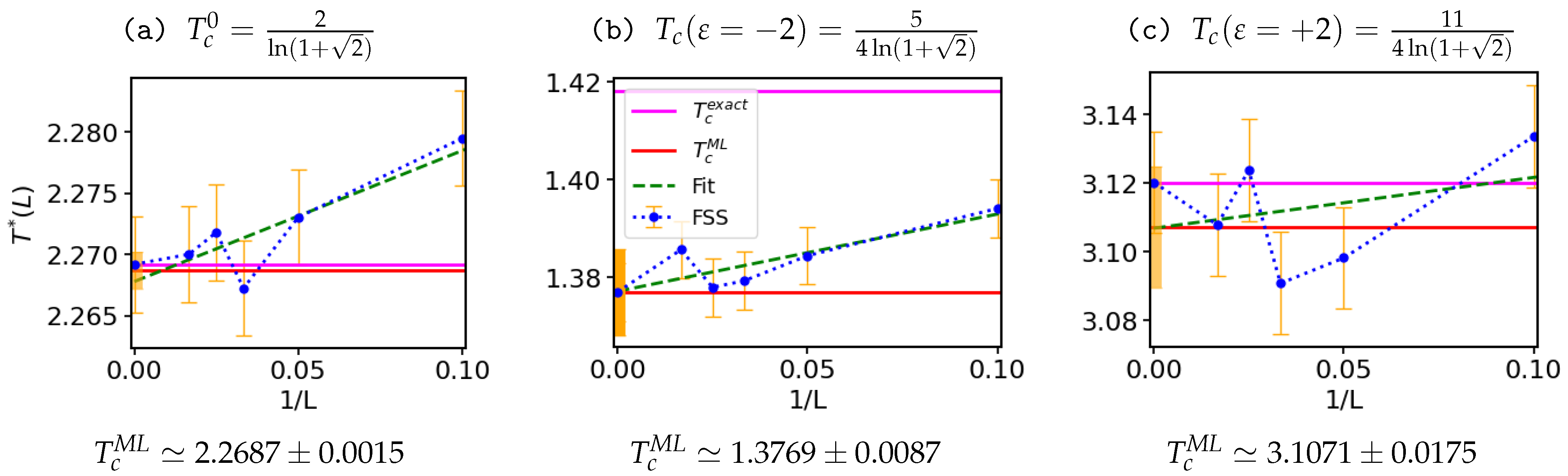
Appendix A.4. Finite Size Scaling of the Transition Temperature

Figure A6 demonstrates the FSS analysis of the crossing temperature T * ( L ) as a function of 1 / L for L = { 10 , 20 , 30 , 40 , 60 } .
Figure A6. The crossing temperature T * ( L ) as a function of 1 / L , where 1 / L = 0 corresponds to thermodynamic limit ( L ). The horizontal red line (see keys) refers to the numerical T c ML (Table 1), and the magenta line represents T c exact (Equation (A5b)) as shown in each panels−(ac).
Condensedmatter 08 00083 g0a6
The horizontal red line (see keys) refers to the numerical T c ML (Table 1), and the magenta line represents the critical temperature in the thermodynamic limit that is calculated using Equation (A5b), T c ( ε = ± 2 ) = ( 16 + 3 ε ) / 8 ln ( 1 + 2 ) , where the known result of T c ( ε = 0 ) is shown for reference. The size of the error bars is equal to one standard deviation of statistical uncertainty. The numerical results are as follows: (a) T c 0 2.2687 ( 15 ) , (b) T c 1.3769 ( 87 ) and (c) T c 3.1071 ( 175 ) are almost in agreement with our solution (A5b). For ε = 2 , the discrepancy is mainly related to the impact of Δ E = 0 in the update rule. For ε < 0 , it is noticed that the function of Δ E = 0 in rule (5) contradicts our argument in Equation (A4). Consequently, the limitation of the modified algorithm for ε < 0 (Appendix A.3) affects the accuracy of the model prediction. The critical exponents ν and β are estimated as discussed in the main part (Section 3; see Figure 3). Furthermore, the estimation of the critical exponent γ can be performed using the FSS theory χ ( T / T c 1 ) γ , where χ represents the latent susceptibility [16]. If z ˜ denotes average absolute latent variable ( z ˜ = | z | ), one can calculate χ as
χ = N z ˜ 2 z ˜ 2 T ,
recalling N = L × L and defining z ˜ = 1 M k = 1 M | z k | , where M is the total number of configurations and k = { 1 , , M } .
Figure A7 demonstrates the latent variable z as a function of T for the given configurations. As a result, one can estimate γ using the result of Equation (A6) where z ˜ can be obtained from the data presented in Figure A7 by plotting χ L γ / ν versus ( T T c 0 ) L 1 / ν . Therefore, it is straightforward to apply this method to the nonequilibrium case ( ε 0 ). Figure A8 shows the latent variable z as a function of T (a) ε = 2 and (b) ε = + 2 .
Figure A7. Scatter plots of the latent variable z versus T for four systems of each linear size L shown at the upper right. This is the case of equilibrium ( ε = 0 ) model. The blue dashed line within each system denotes T c 0 = 2 / ln ( 1 + 2 ) . A gradient color at the right panel illustrates the temperature T, and it reflects the nature of the phase diagram as we move from low T ( T < T c 0 ) to high T ( T > T c 0 ).
Condensedmatter 08 00083 g0a7
Figure A8. Scatter plots of the latent variable z versus T for the given linear size, ε = 2 (upper panel) and ε = + 2 (lower panel). Here, the blue dashed lines denote (a) T c ( ε ) = ( 5 / 4 ) / ln ( 1 + 2 ) and (b) T c ( ε ) = ( 11 / 4 ) / ln ( 1 + 2 ) . The gradient color shown for each panel demonstrates the nature of the phase diagram from the low T ( T < T c ) to the high T ( T > T c ).
Condensedmatter 08 00083 g0a8

References

  1. Kardar, M. Lattice systems. In Statistical Physics of Fields; Cambridge University Press: Cambridge, UK, 2007; pp. 88–122. [Google Scholar]
  2. Nishimori, H.; Ortiz, G. Elements of Phase Transitions and Critical Phenomena; Oxford University Press: New York, NY, USA, 2011. [Google Scholar]
  3. Goldenfeld, N. Lectures on Phase Transitions and The Renormalization Group; CRC Press: Boca Raton, FL, USA, 2018. [Google Scholar]
  4. Linares, J.; Cazelles, C.; Dahoo, P.-R.; Boukheddaden, K. A First Order Phase Transition Studied by an Ising-Like Model Solved by Entropic Sampling Monte Carlo Method. Symmetry 2021, 13, 587. [Google Scholar] [CrossRef]
  5. Derrida, B. Non-equilibrium steady states: Fluctuations and large deviations of the density and of the current. J. Stat. Mech. 2007, 2007, P07023. [Google Scholar] [CrossRef]
  6. Derrida, B. Microscopic versus macroscopic approaches to non-equilibrium systems. J. Stat. Mech. 2011, 2011, P01030. [Google Scholar] [CrossRef]
  7. Bertini, L.; De Sole, A.; Gabrielli, D.; Jona-Lasinio, G.; Landim, C. Macroscopic fluctuation theory. Rev. Mod. Phys. 2015, 87, 593. [Google Scholar] [CrossRef]
  8. Godreche, C.; Bray, A.J. Nonequilibrium stationary states and phase transitions in directed Ising models. J. Stat. Mech. 2009, 2009, P12016. [Google Scholar] [CrossRef]
  9. Stinchcombe, R. Stochastic non-equilibrium systems. Adv. Phys. 2010, 50, 431–496. [Google Scholar] [CrossRef]
  10. Mukamel, D. Nonequilibrium Dynamics, Metastability and Flow. In Soft and Fragile Matter; Cates, M.E., Evans, R., Eds.; CRC Press: Boca Raton, FL, USA, 2000; p. 237. [Google Scholar]
  11. Odor, G. Universality classes in nonequilibrium lattice systems. Rev. Mod. Phys. 2004, 76, 663. [Google Scholar] [CrossRef]
  12. Hinrchsen, H. Non-equilibrium critical phenomena and phase transitions into absorbing states. Adv. Phys. 2000, 49, 815. [Google Scholar] [CrossRef]
  13. Alpaydin, E. Introduction to Machine Learning, 4th ed.; MIT Press: Cambridge, MA, USA, 2004. [Google Scholar]
  14. Tanaka, A.; Tomiya, A. Detection of phase transition via convolutional neural networks. J. Phys. Soc. Jpn. 2017, 86, 063001. [Google Scholar] [CrossRef]
  15. Walker, N.; Tam, K.M.; Novak, B.; Jarrell, M. Identifing structural changes with unsupervised machine learning methods. Phys. Rev. E 2018, 98, 053305. [Google Scholar] [CrossRef]
  16. Alexandrou, C.; Athenodorou, A.; Chrysostomou, C.; Paul, S. The critical temperature of the 2D-Ising model through Deep Learning Autoencoders. Eur. Phys. J. B 2020, 93, 226. [Google Scholar] [CrossRef]
  17. Burak, C.; Romer Rudolf, A.; Honecker, A. Machine Learning the Square-Lattice Ising Model. J. Phys. Conf. Series 2022, 2207, 012058. [Google Scholar]
  18. Huembeli, P.; Dauphin, A.; Wittek, P. Identifing quantum phase transition with adversarial neural networks. Phys. Rev. B 2018, 97, 134109. [Google Scholar] [CrossRef]
  19. Dong, X.Y.; Pollmann, F.; Zhang, X.F. Machine learning of quantum phase transitions. Phys. Rev. B 2019, 99, 121104. [Google Scholar] [CrossRef]
  20. Ohtsuki, T.; Ohtsuki, T. Deep Learning the Quantum Phase Transitions in Random Two-Dimensional Electron Systems. J. Phys. Soc. Jpn. 2016, 85, 123706. [Google Scholar] [CrossRef]
  21. Ohtsuki, T.; Mano, T. Drawing Phase Diagrams of Random Quantum Systems by Deep Learning the Wave Functions. J. Phys. Soc. Jpn. 2020, 89, 022001. [Google Scholar] [CrossRef]
  22. Pilania, G.; Wang, C.; Jiang, X.; Rajasekaran, S.; Ramprasad, R. Accelerating materials property predictions using machine learning. Sci. Rep. 2013, 3, 2810. [Google Scholar] [CrossRef] [PubMed]
  23. Onsager, L. Crystal Statistics. I. A Two Dimensional Model with an Order-Disorder Transition. Phys. Rev. 1944, 65, 117–149. [Google Scholar] [CrossRef]
  24. Yang, C.N.; Lee, L.D. Statistical theory of equations of state and phase transitions: I. Theory of condensation. Phys. Rev. 1952, 87, 404. [Google Scholar] [CrossRef]
  25. Lee, L.D.; Yang, C.N. Statistical theory of equation of state and phase transition: II. Lattice gas and Ising model. Phys. Rev. 1952, 87, 410. [Google Scholar] [CrossRef]
  26. Morningstar, A.; Melko, R.G. Deep Learning the Ising Model Near Criticality. J. Mach. Learn. Res. 2018, 18, 1–17. [Google Scholar]
  27. Walker, N.; Tam, K.M.; Jarrell, M. Deep learning on the 2-dimensional Ising model to extract the crossover region with a variational autoencoder. Sci. Rep. 2020, 10, 13047. [Google Scholar] [CrossRef]
  28. D’Angelo, F.; Böttcher, L. Learning the Ising Model with Generative Neural Networks. Phys. Rev. Res. 2020, 2, 023266. [Google Scholar] [CrossRef]
  29. Carrasquilla, J.; Melko, R.G. Machine learning phases of matter. Nat. Phys. 2017, 13, 431–434. [Google Scholar] [CrossRef]
  30. Corte, I.; Acevedo, S.; Arlego, M.; Lamas, C. Exploring neural network training strategies to determine phase transitions in frustrated magnetic models. Comput. Mater. Sci. 2021, 198, 110702. [Google Scholar] [CrossRef]
  31. Acevedo, S.; Arlego, M.; Lamas, C.A. Phase diagram study of a two-dimensional frustrated antiferromagnet via unsupervised machine learning. Phys. Rev. B 2021, 103, 134422. [Google Scholar] [CrossRef]
  32. Li, Z.; Luo, M.; Wan, X. Extracting critical exponents by finite-size scaling with convolutional neural networks. Phys. Rev. B 2019, 99, 075418. [Google Scholar] [CrossRef]
  33. Burzawa, L.; Liu, S.; Carlson, E.W. Classifying surface probe images in strongly correlated electronic systems via machine learning. Phys. Rev. Mater. 2019, 3, 033805. [Google Scholar] [CrossRef]
  34. Bahri, Y.; Kadmon, J.; Pennington, J.; Schoenholz, S.S.; Sohl-Dickstein, J.; Ganguli, S. Statistical Mechanics of Deep Learning. Annu. Rev. Condens. Matter Phys. 2020, 11, 501–528. [Google Scholar] [CrossRef]
  35. Kumar, M.; Dasgupta, C. Nonequilibrium phase transition in an Ising model without detailed balance. Phys. Rev. E 2020, 102, 052111. [Google Scholar] [CrossRef] [PubMed]
  36. Berg, B. Markov Chain Monte Carlo Simulations and Their Statistical Analysis with Web-Based Fortran Code; World Scientific Publishing Company: Singapore, 2004. [Google Scholar]
  37. Landau, D.P.; Binder, K. A Guide to Monte Carlo Simulations in Statistical Physics, 4th ed.; Cambridge University Press: Cambridge, MA, USA, 2014. [Google Scholar]
  38. Metropolis, N.; Rosenbluth, A.W.; Rosenbluth, M.N.; Teller, A.H.; Teller, E. Equation of State Calculations by Fast Computing Machines. J. Chem. Phys. 1953, 21, 1087–1092. [Google Scholar] [CrossRef]
  39. Janke, W. Introduction to Simulation Techniques; Lecture Notes in Physics 716; Springer: Berlin/Heidelberg, Germany, 2007; pp. 207–260. [Google Scholar]
  40. Abadi, M.; Agarwal, A.; Barham, P.; Brevdo, E.; Chen, Z.; Citro, C.; Corrado, G.S.; Davis, A.; Dean, J.; Devin, M.; et al. TensorFlow: Large-Scale Machine Learning on Heterogeneous Systems. 2015. Available online: https://download.tensorflow.org/paper/whitepaper2015.pdf (accessed on 30 August 2023).
  41. Glauber, R.J. Time-Dependent Statistics of the Ising Model. J. Math. Phys. 1963, 4, 294. [Google Scholar] [CrossRef]
  42. Zia, R.K.P.; Schmittmann, B. Probablity currents as principal characterstics in the statistical mechanics of non-equilibrium steady states. J. Stat. Mech. 2007, 2007, P07012. [Google Scholar] [CrossRef]
  43. Wordofa, D.; Bekele, M. Machine Learning of Nonequilibrium Phase Transition in an Ising Model on Square Lattice. arXiv 2023, arXiv:2307.11901. [Google Scholar] [CrossRef]
Figure 2. Machine learning (ML) the equilibrium ( ε = 0 ) ferromagnetic Ising spin on square-lattice (linear sizes L = 10 , 20 , 40 and 60). (a) The prediction P versus temperature T where the vertical dashed line denotes the estimated value of T c 0 2.2687 ± 0.0015 of the model. (b) A plot showing data collapse of P L β / ν versus ( T T c 0 ) L 1 / ν . The insets represent FM corves and PM corves as shown.
Condensedmatter 08 00083 g002
Figure 3. ML the nonequilibrium ( ε 0 ) ferromagnetic Ising spin on square-lattice ( L = 10 , 20 , 40 and 60), where ε = 2 (a) and ε = + 2 (c). The left panel (a,c) display P versus T while the right panel (b,d) represent the corresponding data collapse P L β / ν versus ( T T c ) L 1 / ν . The estimated values are indicated by dashed lines: T c 1.3769 ± 0.0087 (a), and T c 3.1071 ± 0.0175 (c).
Condensedmatter 08 00083 g003
Disclaimer/Publisher’s Note: The statements, opinions and data contained in all publications are solely those of the individual author(s) and contributor(s) and not of MDPI and/or the editor(s). MDPI and/or the editor(s) disclaim responsibility for any injury to people or property resulting from any ideas, methods, instructions or products referred to in the content.

