The Transport and Optical Characteristics of a Metal Exposed to High-Density Energy Fluxes in Compressed and Expanded States of Matter

Abstract

This article presents a theoretical study of the optical and transport properties of metals. Iron, as an example, was used to discuss, through a theoretical description, the peculiarities of these properties in the compressed and expanded states under the influence of high-density energy fluxes. By solving the semi-classical Boltzmann equation for conduction electrons for a broad range of densities and temperatures, the expressions of electrical conductivity, electronic thermal conductivity, and thermoelectric coefficient calculations were derived. The real and imaginary parts of the iron permittivity and the energy absorption coefficient for the first and second harmonics of Nd:YAG laser radiation were obtained. The calculation peculiarities of the metal’s optical characteristics of matter in an expanded state in a broad range of densities and temperatures were considered. The analysis of the obtained results shows their agreement with the theoretical description for cases of ideal non-degenerate and dense degenerate electron plasmas. It is shown that the behavior of the electrical conductivity and optical characteristics in the critical and supercritical regions of density and temperature are in agreement with the known experimental results.

1. Introduction

This paper presents the development of our initially proposed and published model [1]. The peculiarities of the theoretical description of the thermodynamic properties of a metal accounting for the phase transitions (PTs) of metal–liquid, liquid–gas, and metal–insulator occurring within a wide range of densities and temperatures are studied. The study of electronic transport and optical properties is the main objective of this paper. The non-equilibrium properties of matter in various aggregate states are studied within the framework of the classical kinetic theory formulated in the works of J.K. Maxwell [2], L. Boltzmann [3], and G.A. Lorenz [4], which is still in active development. Since these works were published, the number of papers has increased, and the field of knowledge has expanded so much that we must apologize to those investigators whose papers we do not mention. The current state of the methods of theoretical study for these properties of matter is shown well for condensed matter in [5,6,7,8,9,10,11,12] and for dense gases and non-ideal plasma in [13,14,15,16,17,18,19,20]. A distinctive trend of modern theoretical research is the development of ab initio computer techniques for transport and optical property calculations, e.g., [9,10,11,12,17,18,19,20] and the references therein. Despite tremendous progress in computer technology and calculation speed growth, these methods still require considerable computer resources to obtain significant results. Hence, these techniques do not cancel out the theoretical–analytical approach. Therefore, in the proposed work, we study the properties of a metal based on the solution of the semi-classical Boltzmann kinetic equation for conduction electrons, written in reference to a quasi-neutral atomic cell [21]. We used well-known analytical methods (see [21,22,23,24,25] and the references therein) to find the solution to this equation. Considerable attention was paid to determining the mean free path of electrons and considering its relationship with the thermophysical properties of the metal in our earlier works [21,22,24]. The unique quality of our approach, as outlined in our previous article [1], is the joint description of the thermal and electrical processes occurring in the expanded and compressed metal. The metal model proposed in this paper makes it possible to determine thermodynamic functions while accounting for the PTs. The model has limitations in accounting for PTs’ influence on the expanded state alone. The effect of structure and PTs during compression require a separate study.

2. Results

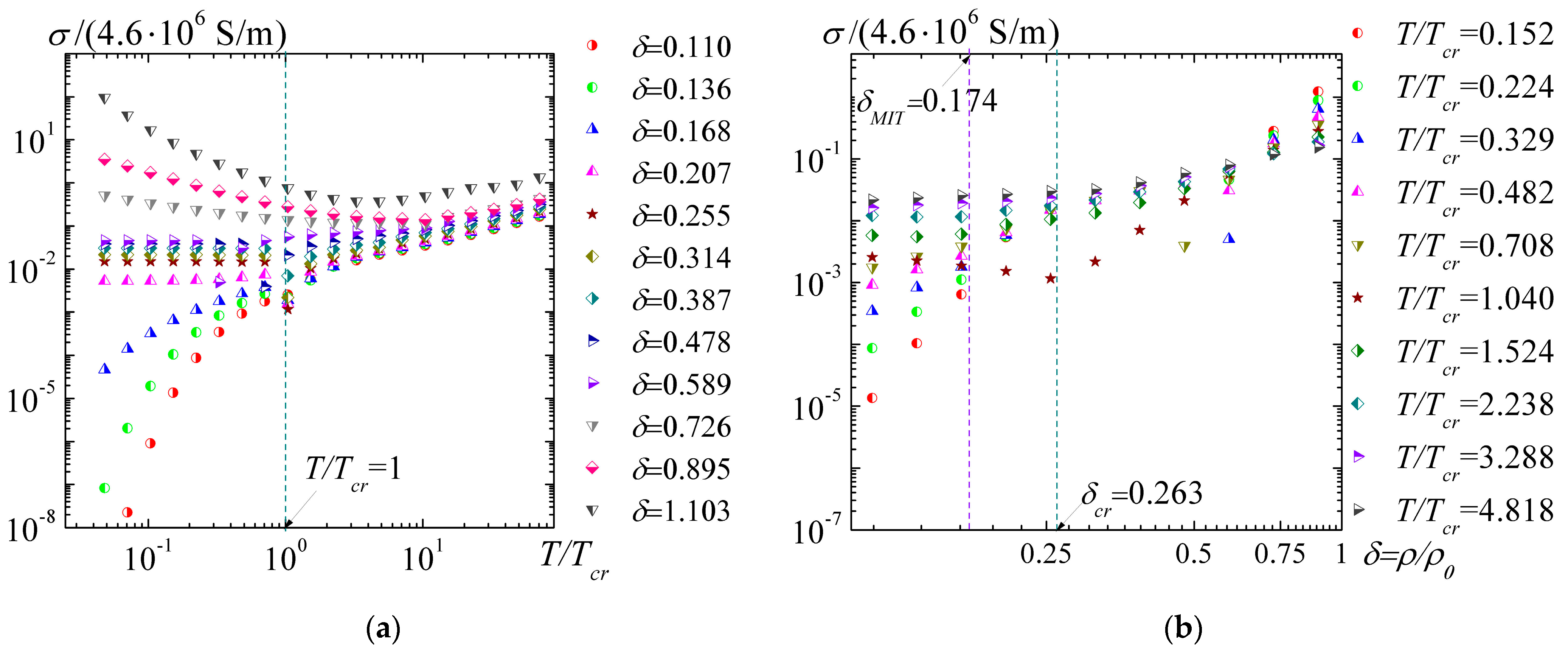
2.1. Transport Properties of Metal in a Quasi-Stationary Electromagnetic Field

Here, we use the known plasma model of a metal [22,24,26] for the calculation of the electronic kinetic coefficients in a compressed and expanded state, i.e., we consider the metal to be a plasma-like medium with a symmetric part of the distribution function of the conduction electrons conforming to Fermi–Dirac statistics [27]. One can write the generalized Ohm and Fourier laws in the center of the mass reference frame of a quasi-neutral atomic cell [21] as follows [24,28]:

$$E+\frac{1}{e}\nabla {\mu }_1=\frac{1}{M_{00}}j+\alpha \nabla T;$$

(1)

$$q=\frac{{\mu }_1{K}_{00}-e{K}_{01}}{{\mu }_1{M}_{00}-e{M}_{01}}\alpha Tj-\frac{{\mu }_1}{e}j-\kappa \nabla T.$$

(2)

Here, E is the electric field, j is the current density, q is the density of the electron heat flow, μ₁(V_a,T) is the chemical potential of the conduction electrons (see [1] and the references therein), and α(V_a,T) is the thermoelectric coefficient, defined as follows:

$$\alpha =\frac{1}{eT}\left({\mu }_1-\frac{e{M}_{01}}{M_{00}}\right)$$

(3)

The electronic thermal conductivity κ(V_a,T) is defined as follows:

$$\kappa =\frac{K_{00}}{eT}\left(\frac{M_{01}}{M_{00}}\left({\mu }_1-\frac{e{K}_{01}}{K_{00}}\right)-\frac{K_{01}}{K_{00}}\left({\mu }_1-\frac{e{K}_{02}}{K_{01}}\right)\right)$$

(4)

M_oi(V_a,T) and K_oi(V_a,T), i = 0, 1, 2, are the Onsager kinetic coefficients, and e, V_a, and T are the electron charge, the volume of an atomic cell, and the temperature, respectively.

Using well-known analytical methods [21,22,23,24,25], one can obtain expressions for the Onsager coefficients by solving the semi-classical Boltzmann equation for conduction electrons. In the SGS system, they will be as follows:

$$\begin{array}{l}{M}_{0\beta }=\frac{2m{e}^{2-\beta }}{3{\pi }^2{ħ}^3}\frac{\partial }{\partial {\mu }_1}{\displaystyle {\int }_0^{\infty }{\epsilon }^{\beta +1}{l}_{j,eff}(\epsilon ){\left(\exp ((\epsilon -{\mu }_1)/T)+1\right)}^{-1}}d\epsilon =\\ \hspace{1em}\hspace{1em}=\frac{2}{3{\pi }^2{e}^{\beta }ħ}{\left(\frac{m{e}^4}{{ħ}^2}\right)}^{\beta +1}{\overline{T}}^{\beta +1}\frac{\partial }{\partial x}{\displaystyle {\int }_0^{\infty }{\xi }^{\beta +1}{\overline{l}}_{j,eff}(\xi )f_0\left(\xi -x\right)}d\xi =\\ \hspace{1em}\hspace{1em}=\frac{1}{e^{\beta }ħ}{E}_H{}^{\beta +1}{\overline{M}}_{0\beta },\hspace{0.17em}\beta =0,1,2;E_H=\frac{m{e}^4}{{ħ}^2},\xi =\frac{\epsilon }{T}=\frac{\overline{\epsilon }}{\overline{T}},\\ \hspace{1em}\hspace{1em}x=\frac{{\mu }_1}{T}=\frac{{\overline{\mu }}_1}{\overline{T}},\overline{T}=\frac{T}{E_H},{\overline{\mu }}_1=\frac{{\mu }_1}{E_H},{\overline{l}}_{j,eff}=\frac{l_{j,eff}}{a_B},a_B=\frac{{ħ}^2}{m{e}^2};\end{array}$$

(5)

$$\begin{array}{l}{K}_{0\beta }=\frac{2m{e}^{2-\beta }}{3{\pi }^2{ħ}^3}\frac{\partial }{\partial {\mu }_1}{\displaystyle {\int }_0^{\infty }{\epsilon }^{\beta +1}{l}_{q,eff}(\epsilon ){\left(\exp ((\epsilon -{\mu }_1)/T)+1\right)}^{-1}}d\epsilon =\\ \hspace{1em}\hspace{0.17em}\hspace{0.17em}\hspace{0.17em}=\frac{2}{3{\pi }^2{e}^{\beta }ħ}{\left(\frac{m{e}^4}{{ħ}^2}\right)}^{\beta +1}{\overline{T}}^{\beta +1}\frac{\partial }{\partial x}{\displaystyle {\int }_0^{\infty }{\xi }^{\beta +1}{\overline{l}}_{q,eff}(\xi )f_0\left(\xi -x\right)}d\xi =\\ \hspace{1em}\hspace{1em}=\frac{1}{e^{\beta }ħ}{E}_H{}^{\beta +1}{\overline{K}}_{0\beta },\hspace{1em}\hspace{1em}\beta =0,1,2;{\overline{l}}_{q,eff}=\frac{l_{q,eff}}{a_B}.\end{array}$$

(6)

Here, in relation to (5) and (6),

$$\begin{array}{l}{\overline{M}}_{0\beta }=\frac{2}{3{\pi }^2}{\overline{T}}^{\beta +1}\frac{\partial }{\partial x}{\displaystyle {\int }_0^{\infty }{\xi }^{\beta +1}{\overline{l}}_{j,eff}(\xi )f_0\left(\xi -x\right)}d\xi ,\hspace{0.17em}\beta =0,1,2;\\ {\overline{K}}_{0\beta }=\frac{2}{3{\pi }^2}{\overline{T}}^{\beta +1}\frac{\partial }{\partial x}{\displaystyle {\int }_0^{\infty }{\xi }^{\beta +1}{\overline{l}}_{q,eff}(\xi )f_0\left(\xi -x\right)}d\xi ,\hspace{0.17em}\beta =0,1,2;\end{array}$$

(7)

E_H = me⁴ħ⁻² and a_B = ħ²/(me²) are the Hartree energy and the Bohr radius. Also, l_j,eff(ε) and l_q,eff(ε) are the electrons’ mean free paths responsible for an electric current and a heat transfer in a matter. These values are represented in the system of atomic units (SAU) [29].

Table A1. Brief information about some physical quantities in the system of atomic units.

Unit Symbol and Definition	SGS	SI
Light velocity: c	2.99792458 × 1010 cm/s	2.99792458 × 108 m/s
Boltzmann constant: kB	1.3806505 × 10−16 erg/K	1.3806505 × 10−23 J/K
Reduced Planck constant: $ħ$	1.05457168 × 10−27 erg$·$s	1.05457168 × 10−27 J$·$s
Electron mass: m	9.1093826 × 10−28 g	9.1093826 × 10−31 kg
Electron rest energy: E0 = mc2	8.187104787 × 10−7 erg	8.187104787 × 10−14 J
Fine structure constant: αFSC	7.297352568 × 10−3	7.297352568 × 10−3
Elementary charge: e	4.80332044 × 10−10 GSG	1.60217653 × 10−19 C
Basic energy: EH = αFSC2$·$E0	4.3597442 × 10−11 erg	4.3597442 × 10−18 J
Bohr radius: aB	5.2917721 × 10−11 cm	5.2917721 × 10−9 m
Wavenumber: qB = aB−1	1.889726142 × 108 cm−1	1.889726142 × 1010 m−1
Basic square: Sau = aB2	2.8 × 10−17 cm2	2.8 × 10−21 m2
Basic volume: Vau = aB3	1.481847 × 10−25 cm3	1.481847 × 10−31 m3
Particle concentration: N = 1/Vau	6.748334685 × 1024 cm−3	6.748334685 × 1030 m−3
Basic time: tau = $ħ$/EH	2.4188843 × 10−17 s	2.4188843 × 10−17 s
Basic frequency: ωau = tau−1	4.134137372 × 1016 s−1	4.134137372 × 1016 s−1
Basic velocity: vau = αFSC$·$c	2.187691263 × 108 cm/s	2.187691263 × 106 m/s
Basic force: Fau = EH/aB	8.238722577 × 10−3 dyn	8.238722577 × 10−8 N
Basic pressure: Pau = EH/Vau	294.2101296 Mbar	29.42101296 TPa
Basic current: Iau = evau/aB	1.985710681 × 107 SGS	6.6236178688 × 10−3 A
Basic voltage: Uau = EH/e	0.09076741 SGS	27.211384712 V
Electric strength: Eau = EH/e$·$aB	1.715255461 × 107 SGS	5.142206506 × 1011 V/m
Current density: Jau = Iau/Sau	7.091101703 × 1023 SGS/cm2	2.365336324 × 1018 A/m2
Electric conductivity:
σau = Jau/Eau	4.134137372 × 1016 s−1	4.5998482 × 106 S/m
Thermal conductivity:
κen = 1/(aB$·$tau)	7.812387468 × 1024 (cm$·$s)−1	7.812387468 × 1026 (m$·$s)−1
κau = κen$·$kB	1.07861767 × 109 erg/(s$·$cm$·$K)	1.07861767 × 104 W/(m$·$K)
Thermal power: αau = kB/e	2.87443628 × 10−7 erg/(K$·$SGS)	8.61734318 × 10−5 J/(C$·$K)

of Appendix A provides brief information about this system that is necessary for understanding it. Using the normalization condition of the Fermi–Dirac function (see expression (29) in [1]), one can represent relation (7) as follows:

$$\begin{array}{l}{\overline{M}}_{0\beta }=\frac{\sqrt{2}{z}_i{\overline{n}}_i{\overline{T}}^{\beta -1/2}}{3}\frac{\frac{\partial }{\partial x}{\displaystyle {\int }_0^{\infty }{\xi }^{\beta +1}{\overline{l}}_{j,eff}(\xi )f_0(\xi -x)d\xi }}{F_{1/2}(x)},\\ {\overline{K}}_{0\beta }=\frac{\sqrt{2}{z}_i{\overline{n}}_i{\overline{T}}^{\beta -1/2}}{3}\frac{\frac{\partial }{\partial x}{\displaystyle {\int }_0^{\infty }{\xi }^{\beta +1}{\overline{l}}_{q,eff}(\xi )f_0(\xi -x)d\xi }}{F_{1/2}(x)},{\overline{n}}_i=\frac{a_B{}^3}{V_a}=1/{\overline{V}}_a.\end{array}$$

(8)

Here, z_i is the number of conduction electrons per atomic cell or the average ion charge, and $z_i{\overline{n}}_i$ is their concentration. $F_{\nu }(x)={\displaystyle {\int }_0^{\infty }{(\exp (\xi -x)+1)}^{-1}{\xi }^{\nu }d\xi }\hspace{1em}(\nu >-1)$ is the Fermi–Dirac function.

Taking into account relations (5)–(8), one can write Equations (1) and (2) in dimensionless form as follows:

$$\begin{array}{l}\overline{E}+\overline{\nabla }{\overline{\mu }}_1=\frac{1}{{\overline{M}}_{00}}\overline{j}+\overline{\alpha }\overline{\nabla }\overline{T},\hspace{0.17em}\overline{E}=E/E_{au}, E_{au}=E_H/(e{a}_B), \overline{\alpha }=\alpha /e;\\ \overline{q}=\left(\frac{x{\overline{K}}_{00}-{\overline{K}}_{01}/\overline{T}}{x{\overline{M}}_{00}-{\overline{M}}_{01}/\overline{T}}\overline{\alpha }-x\right)\overline{T}\overline{j}-\overline{\kappa }\overline{\nabla }\overline{T},\overline{q}=\frac{q}{q_{au}},q_{au}=\frac{E_H{}^2}{ħa_B{}^2},\overline{\kappa }=\frac{\kappa }{{\kappa }_{au}},{\kappa }_{au}=\frac{E_H}{ħa_B}.\end{array}$$

(9)

The thermoelectric coefficient $\overline{\alpha }$ and electronic thermal conductivity $\overline{\kappa }$ in (9) have the following form:

$$\begin{array}{l}\overline{\alpha }=x-\frac{{\overline{M}}_{01}}{\overline{T}{\overline{M}}_{00}}=x-\frac{\frac{\partial }{\partial x}{\displaystyle {\int }_0^{\infty }{\xi }^2{\overline{l}}_{j,eff}(\xi )f_0(\xi -x)d\xi }}{\frac{\partial }{\partial x}{\displaystyle {\int }_0^{\infty }\xi {\overline{l}}_{j,eff}(\xi )f_0(\xi -x)d\xi }};\\ \overline{\kappa }=\frac{1}{\overline{T}}\left({\overline{K}}_{02}-\frac{{\overline{M}}_{01}{\overline{K}}_{01}}{{\overline{M}}_{00}}\right)+x\left(\frac{{\overline{K}}_{00}{\overline{M}}_{01}}{{\overline{M}}_{00}}-{\overline{K}}_{01}\right).\end{array}$$

(10)

As follows from the relations above, it is necessary to determine the calculation method of the two mean free paths, ${\overline{l}}_{j,eff}$ and ${\overline{l}}_{q,eff}$, in order to calculate the transport characteristics of a metal, particularly iron. Here, we will divide the metal in an expanded state (δ = V_a0/V_a = ρ/ρ₀ < 1) from the compressed one (δ ≥ 1). In the expanded state, both of these mean free paths are equal. In the compressed state, the heat transfer by electrons at temperatures lower than the Debye temperature is more favorable in the transition of electrons from the states above the Fermi surface to the states below it than due to the diffusion along its surface [30,31]. To find the mean free path, similar to [21,22,24], we will use the fundamental relation of the diffraction model of the metal [32], which J. I. Frenkel used in the 1920s to explain the dependence of electrical conductivity on temperature. Its essence is the analogy between the scattering of conduction electrons and light on density fluctuations as follows [33]:

$$l_j{}^{-1}=\frac{m^2{n}_i}{4\pi {ħ}^4{k}^4}{{\displaystyle {\int }_0^{2k}{S}_i{}^2(q)\left|\langle k+q|w_i|k\rangle \right|}}^2\epsilon {(q)}^{-2}{q}^{3}dq$$

(11)

Here, in (11), k = (2mε_e)^1/2/ħ is the wavenumber of the conduction electron with energy ε_e and mass m. S_i²(q) is the square of the ionic static structural factor of metallic plasma (for an ideal gas of ions (atoms) S_i²(q) = 1). In the long-wavelength approximation, S_i²(q) is as follows [21,22,24]:

$$S_i{}^2(0)=S_{ii}{}^{-1},\hspace{0.17em}{S}_{ii}=\frac{{{\rm K}}_{ii}(\rho ,T)}{n_{i}T}$$

(12)

Here, Κ_ii = ρ∂P_i/∂ρ∣_T is the modulus of isothermal compressibility of an ionic metal component, ∣〈k + q|w_i|k〉∣² is the squared form factor of unshielded ions or atoms, ε(q) = 1 + k_D²q⁻² is the static permittivity of the Debye plasma, k_D² = min{k_s², k_ei²} is the squared Debye wavenumber of plasma, k_s = r_s⁻¹, r_s = (3/4πn_i)^1/3 is the average interatomic distance, k_ei2 = k_De² + (k_Di⁴ + k_s⁴)k_D⁻², k_Di² = 4πe²z_i²n_i²/T is the squared Debye wavenumber of an ion, and k_De² = 2πe²z_in_iF_−1/2(μ₁/T)/F_1/2(μ₁/T) is the squared Debye wavenumber of an electron. To find the form factor of an unshielded ion, one has to use the effective potential of an ion as follows [21,22,24]:

$$w_i\left(r\right)=-\frac{e^2{z}_i}{r}+\frac{e^2\left(Z-z_i\right)}{r}\exp \left(-\frac{r}{r_c}\right),\hspace{0.17em}{r}_c=\frac{Z-z_i}{Z^{3/2}}{\left(\frac{{\langle r^2\rangle }_a}{6}\right)}^{1/2}$$

(13)

where r_c is the shielding radius of the internal electron, and the values of 〈r_c〉_a are averaged over the electronic density of the atom [34]. Similarly to [32], one can obtain the expression for the squared form factor for the case of a spherically symmetric potential (13) as follows:

$${\left|\langle k+q|w_i|k\rangle \right|}^2=16{\pi }^2{e}^4\left(\frac{z_i{}^2}{q^4}+\frac{{\left(Z-z_i\right)}^2{r}_c{}^4}{{\left(1+q^2{r}_c{}^2\right)}^4}\right).$$

(14)

It is supposed for expression (14) that the main contribution to the mean free path is defined by the scattering of conduction electrons on the internal electrons of the atom when z_i << Z (see [21,22,24] and the references therein). The contribution of the second term in the potential (13) and its form factor to the mean free path is significant for considering the weakly ionized substance (z_i << Z) in the expanded state (δ < 1). The accounting of scattering by an atom’s internal electrons in the compressed state requires separate investigations. That is why in this paper, for the first approximation, we will neglect it for simplicity.

It is known [30] that for the compressed state, the cutoff factor is the Debye wavenumber q_D = (6π ²/V_a)^1/3 = q_D0δ^1/3 [1]. The structural factor for the compressed state of a metal can be represented as follows [24]:

$$S_i{}^2(q)=S_{ii}{}^{-1}\frac{\frac{q}{q_D}\frac{\Theta }{T}}{\exp \left(\frac{q}{q_D}\frac{\Theta }{T}\right)-1}=S_{ii}{}^{-1}\frac{\frac{q}{q_D}\frac{ħ{\omega }_D}{T}}{\exp \left(\frac{q}{q_D}\frac{ħ{\omega }_D}{T}\right)-1}$$

(15)

Here, in (15), Θ = ħω_D is the Debye temperature of a metal in a compressed state. It depends on the density (volume of atom cell) [1]. Given the above, we can write the expression for the dimensionless mean free path used in (8)–(10) in the form as follows:

$${\overline{l}}_j\left({\overline{\epsilon }}_e\right)=\frac{{\overline{\epsilon }}_e{}^2{S}_{ii}\left({\overline{n}}_i,\overline{T}\right)}{\pi {\overline{n}}_i{\Lambda }_j\left(\langle {\overline{\epsilon }}_e\rangle \right)}$$

(16)

where

$${\Lambda }_j\left(\langle {\overline{\epsilon }}_e\rangle \right)=\{\begin{array}{l}{z}_i{}^2{\Lambda }_{j,c}\left(\langle {\overline{\epsilon }}_e\rangle \right)\hspace{0.17em}\mathrm{for}\hspace{0.17em}{\overline{V}}_a\le {\overline{V}}_{a0}\hspace{0.17em}(\delta ={\overline{V}}_{a0}/{\overline{V}}_a\ge 1);\\ z_i{}^2{\Lambda }_{j,ex1}\left(\langle {\overline{\epsilon }}_e\rangle \right)+{\left(Z-z_i\right)}^2{\Lambda }_{j,ex2}\left(\langle {\overline{\epsilon }}_e\rangle \right)\hspace{0.17em}\mathrm{for}\hspace{0.17em}{\overline{V}}_a>{\overline{V}}_{a0}\hspace{0.17em}(\delta <1).\end{array}$$

(17)

Here, in (17), ${\Lambda }_{j,c}\left(\langle {\overline{\epsilon }}_e\rangle \right)$, ${\Lambda }_{j,ex1}\left(\langle {\overline{\epsilon }}_e\rangle \right)$, and ${\Lambda }_{j,ex2}\left(\langle {\overline{\epsilon }}_e\rangle \right)$ are the analogs of the Coulomb logarithms. They are widely used to describe the transport properties of ideal plasma.

$${\Lambda }_{j,c}\left(\langle {\overline{\epsilon }}_e\rangle \right)=b_1{}^4{\displaystyle {\int }_0^{{(8<{\overline{\epsilon }}_e>)}^{1/2}{\overline{\omega }}_D/{\overline{q}}_D\overline{T}}\frac{{\zeta }^{4}d\zeta }{\left(\exp \left(\zeta \right)-1\right){\left(1+b_1{}^2{\zeta }^2\right)}^2}},\hspace{0.17em}{b}_1=\frac{{\overline{q}}_D}{{\overline{k}}_D}\frac{\overline{T}}{{\overline{\omega }}_D}$$

(18)

$${\Lambda }_{j,ex1}\left(\langle {\overline{\epsilon }}_e\rangle \right)={\displaystyle {\int }_0^{{(8<{\overline{\epsilon }}_e>)}^{1/2}/{\overline{k}}_D}\frac{{\zeta }^{3}d\zeta }{{\left(1+{\zeta }^2\right)}^2}}$$

(19)

$${\Lambda }_{j,ex2}\left(\langle {\overline{\epsilon }}_e\rangle \right)=b_2{}^4{\displaystyle {\int }_0^{{(8<{\overline{\epsilon }}_e>)}^{1/2}/{\overline{k}}_D}\frac{{\zeta }^{7}d\zeta }{{\left(1+b_2{}^2{\zeta }^2\right)}^2{\left(1+{\zeta }^2\right)}^2}},\hspace{0.17em}{b}_2={\overline{r}}_c{\overline{k}}_D$$

(20)

To reduce the calculation difficulties of the kinetic coefficients, these integrals in (18)–(20) will be defined with the use of the average energy of the conduction electron. For the case under investigation, this energy is only the function of the temperature and volume of the atomic cell.

Then, the mean free path l_q, which defines the heat transferred by electrons, is given by the following relation:

$${\overline{l}}_q({\overline{\epsilon }}_e)=\frac{{\overline{\epsilon }}_e{}^2{S}_{ii}({\overline{n}}_i,\overline{T})}{\pi {\overline{n}}_i{\Lambda }_q\left(\langle {\overline{\epsilon }}_e\rangle \right)}$$

(21)

Based on the conclusions made in [24,31], ${\Lambda }_q\left(\langle {\overline{\epsilon }}_e\rangle \right)$ can be written as follows:

$${\Lambda }_q\left(\langle {\overline{\epsilon }}_e\rangle \right)=\{\begin{array}{l}{z}_i{}^2{\Lambda }_{j,c}\left(\langle {\overline{\epsilon }}_e\rangle \right)\left(1+3{\pi }^{-2}{\left({\overline{k}}_F{\overline{q}}_D{}^{-1}\right)}^2{\left({\overline{\omega }}_D{\overline{T}}^{-1}\right)}^2\right)\hspace{0.17em}\mathrm{for}\hspace{0.17em}{\overline{V}}_a\le {\overline{V}}_{a0}\hspace{0.17em}(\delta \ge 1);\\ z_i{}^2{\Lambda }_{j,ex1}\left(\langle {\overline{\epsilon }}_e\rangle \right)+{\left(Z-z_i\right)}^2{\Lambda }_{j,ex2}\left(\langle {\overline{\epsilon }}_e\rangle \right)\hspace{0.17em}\mathrm{for}\hspace{0.17em}{\overline{V}}_a>{\overline{V}}_{a0}\hspace{0.17em}(\delta <1).\end{array}$$

(22)

In (22), ${\overline{k}}_F={\left(3{\pi }^2{z}_i({\overline{V}}_a,\overline{T}=0)/{\overline{V}}_a\right)}^{1/3}$ is the wavenumber of an electron on the Fermi surface. When $\overline{T}\to {\overline{\omega }}_D$ and ${\overline{V}}_a\le {\overline{V}}_{a0}\hspace{0.17em}(\delta \ge 1)$, it follows from relation (18) that ${\Lambda }_{j,c}\cong 4!b_1{}^4=24{({\overline{q}}_D\overline{T}/{\overline{k}}_D{\overline{\omega }}_D)}^4$. The mean free paths have the following asymptotic behavior for this case:

$$\begin{array}{l}{\overline{l}}_j\left({\overline{\epsilon }}_e\right)=\frac{{\overline{\epsilon }}_e{}^2{S}_{ii}\left({\overline{n}}_i,\overline{T}\right)}{\pi {\overline{n}}_i{\Lambda }_j\left(\langle {\overline{\epsilon }}_e\rangle \right)}=\frac{{\overline{\epsilon }}_e{}^2{S}_{ii}\left({\overline{n}}_i,\overline{T}\right)}{24\pi {\overline{n}}_i{z}_i{}^2{({\overline{q}}_D\overline{T}/{\overline{k}}_D{\overline{\omega }}_D)}^4}\propto \frac{{\overline{\epsilon }}_e{}^2}{{\overline{n}}_i{z}_i{}^2\overline{T}}{\left(\frac{{\overline{k}}_D{\overline{\omega }}_D}{{\overline{q}}_D\overline{T}}\right)}^4\propto {\overline{T}}^{-5};\\ {\overline{l}}_q\left({\overline{\epsilon }}_e\right)=\frac{{\overline{\epsilon }}_e{}^2{S}_{ii}\left({\overline{n}}_i,\overline{T}\right)}{\pi {\overline{n}}_i{\Lambda }_j\left(\langle {\overline{\epsilon }}_e\rangle \right)\left(1+3{\pi }^{-2}{\left({\overline{k}}_F{\overline{q}}_D{}^{-1}\right)}^2{\left({\overline{\omega }}_D{\overline{T}}^{-1}\right)}^2\right)}\cong \frac{\pi {\overline{\epsilon }}_e{}^2{S}_{ii}\left({\overline{n}}_i,\overline{T}\right){\left({\overline{k}}_D{\overline{\omega }}_D\right)}^4}{72{\overline{n}}_i{z}_i{}^2{({\overline{q}}_D\overline{T})}^2{\left({\overline{k}}_F{\overline{\omega }}_D\right)}^2}\propto T^{-3}.\end{array}$$

(23)

The relations obtained above, (16) for ${\overline{l}}_j({\overline{\epsilon }}_e)$ and (21) for ${\overline{l}}_q({\overline{\epsilon }}_e)$, along with the Equations (17)–(20) and (22), allow one to calculate the Onsager electronic kinetic coefficient (8). Therefore, it is possible to determine the electrical $\overline{\sigma }(\delta ,\overline{T})$ and thermal conductivities $\overline{\kappa }(\delta ,\overline{T})$ and thermoelectric coefficient $\overline{\alpha }(\delta ,\overline{T})$ in a broad range of densities and temperatures.

First, it is worth discussing the behavior of the shielding parameters of the ions’ potential and its internal electrons as functions of the volume of an atomic cell and temperature. Figure 1a shows the behavior of the squared Debye wavenumbers of electrons ${\overline{k}}_{De}{}^2({\overline{V}}_a,\overline{T})$ and ions ${\overline{k}}_{Di}{}^2({\overline{V}}_a,\overline{T})$ and ${\overline{k}}_D{}^2({\overline{V}}_a,\overline{T})$ in comparison with the behavior of the squared mean wavenumbers ${\overline{k}}_s{}^2={(3/4\pi {\overline{n}}_i)}^{-2/3}$. The behavior of the squared shielding radius of the inner electrons is shown in Figure 1b.

The left dotted line, which corresponds to the value of ${\overline{V}}_0\equiv {\overline{V}}_{a0}=79.516$, separates the compressed state from the expanded one. The right dotted line with the value of $\overline{V}={\overline{V}}_{MIT}=457.513$ corresponds to the metal–insulator PT boundary. In this case, the overlap of the electron wave functions disappears at zero temperature, i.e., the electrons appear to be localized. This value of the volume in atomic units corresponds to the values of the relative and real density of iron: δ_MIT = 0.174, ρ_MIT = 1.368, g/cm³. The iron parameters corresponding to this critical point were obtained earlier [1]: $\overline{V}={\overline{V}}_{cr}=302.348$, δ_cr = 0.263, ρ_cr = 2.07, g/cm³. The comparison of curves in Figure 1a shows that the Debye screening radius of the ion potential coincides with ${\overline{r}}_s$. The curves in Figure 1b show that ${\overline{r}}_c{}^2$ is practically independent of the temperature up to the critical one. A further increase in the temperature leads to its decrease, which is used to associate with an ionization increase, i.e., a decrease in the number of internal electrons of the ions.

Figure 2 shows the behavior of the long-wavelength structure factor S_ii(δ,T) of iron in dependence on δ for low (a) and high (b) temperatures. As above, the dotted line in Figure 2a,b corresponds to the relative critical density δ_cr = 0.263. An analysis of the curves shows that the figure plotted on a logarithmic scale cannot contain points with a negative value of the structure factor S_ii(δ,T). Strictly speaking, the presence of these negative values shows the limitation of the hydrodynamic approximation in the liquid–gas PT range. It is possible to use the hydrodynamic approximation when the mean free is limited by the following condition: ${\overline{l}}_j\ge {\overline{r}}_s$.

The following modification of expression (8) is proposed for calculating the Onsager coefficients ${\overline{M}}_{0\beta }$ for ${\overline{V}}_a>{\overline{V}}_{a0}(\delta <1)$:

$$\begin{array}{l}{\overline{M}}_{0\beta }=\frac{\sqrt{2}{z}_i{\overline{n}}_i{\overline{T}}^{\beta -1/2}}{3}\frac{\frac{\partial }{\partial x}{\displaystyle {\int }_0^{\infty }{\xi }^{\beta +1}{\overline{l}}_{j,eff}(\xi )f_0(\xi -x)d\xi }}{F_{1/2}(x)}=\\ \hspace{1em}\hspace{1em}=\{\begin{array}{l}\frac{\sqrt{2}{z}_i{\overline{T}}^{\beta +3/2}}{3\pi {\Lambda }_j\left(\langle {\overline{\epsilon }}_e\rangle \right)}\frac{\frac{\partial }{\partial x}{\displaystyle {\int }_0^{\infty }{\xi }^{\beta +3}{f}_0(\xi -x)d\xi }}{F_{1/2}(x)}=\frac{\sqrt{2}{z}_i{\overline{T}}^{\beta +3/2}}{3\pi {\Lambda }_j\left(\langle {\overline{\epsilon }}_e\rangle \right)}\frac{{F^{\prime }}_{\beta +3}\left(x\right)}{F_{1/2}(x)}\hspace{0.17em}\mathrm{for}\hspace{0.17em}{S}_{ii}>0;\\ \frac{\sqrt{2}{z}_i{\overline{n}}_i{\overline{r}}_s{\overline{T}}^{\beta -1/2}}{3}\frac{\frac{\partial }{\partial x}{\displaystyle {\int }_0^{\infty }{\xi }^{\beta +1}{f}_0(\xi -x)d\xi }}{F_{1/2}(x)}=\frac{\sqrt{2}{z}_i{\overline{n}}_i{\overline{r}}_s{\overline{T}}^{\beta -1/2}}{3}\frac{{F^{\prime }}_{\beta +1}\left(x\right)}{F_{1/2}(x)}\hspace{0.17em}\mathrm{for}\hspace{0.17em}{S}_{ii}\le 0.\end{array}\end{array}$$

(24)

The expressions for the electrical conductivity, thermal conductivity, and thermoelectric coefficient will be the following for the case ${\overline{V}}_a>{\overline{V}}_{a0}(\delta <1)$:

$$\overline{\sigma }={\overline{M}}_{00}=\{\begin{array}{l}\frac{\sqrt{2}{z}_i{\overline{T}}^{3/2}}{3\pi {\Lambda }_j\left(\langle {\overline{\epsilon }}_e\rangle \right)}\frac{{F^{\prime }}_3\left(x\right)}{F_{1/2}(x)}=\frac{\sqrt{2}{z}_i{\overline{T}}^{3/2}}{\pi {\Lambda }_j\left(\langle {\overline{\epsilon }}_e\rangle \right)}\frac{F_2\left(x\right)}{F_{1/2}(x)}\hspace{0.17em}\mathrm{for}\hspace{0.17em}{S}_{ii}>0;\\ \frac{\sqrt{2}{z}_i{\overline{n}}_i{\overline{r}}_s}{3{\overline{T}}^{1/2}}\frac{{F^{\prime }}_1\left(x\right)}{F_{1/2}(x)}=\frac{\sqrt{2}{z}_i{\overline{n}}_i{\overline{r}}_s}{3{\overline{T}}^{1/2}}\frac{F_0\left(x\right)}{F_{1/2}(x)}\hspace{0.17em}\mathrm{for}\hspace{0.17em}{S}_{ii}\le 0.\end{array}$$

(25)

$$\overline{\kappa }=\{\begin{array}{l}\frac{\sqrt{2}{z}_i{\overline{T}}^{5/2}{S}_{ii}}{3\pi {\Lambda }_j\left(\langle {\overline{\epsilon }}_e\rangle \right)}\left(\frac{{F^{\prime }}_5(x)}{F_{1/2}(x)}-\frac{{\left({F^{\prime }}_4(x)\right)}^2}{{F^{\prime }}_3(x)F_{1/2}(x)}\right)=\\ =\frac{5\sqrt{2}{z}_i{\overline{T}}^{5/2}{S}_{ii}}{3\pi {\Lambda }_j\left(\langle {\overline{\epsilon }}_e\rangle \right)}\left(\frac{F_4(x)}{F_{1/2}(x)}-\frac{16}{15}\frac{F_3{}^2(x)}{F_2(x)F_{1/2}(x)}\right) \mathrm{for} S_{ii}>0;\\ \frac{\sqrt{2}{z}_i{\overline{n}}_i{\overline{r}}_s{\overline{T}}^{1/2}}{3}\left(\frac{{F^{\prime }}_3(x)}{F_{1/2}(x)}-\frac{{\left({F^{\prime }}_2(x)\right)}^2}{{F^{\prime }}_1(x)F_{1/2}(x)}\right)=\\ =\sqrt{2}{z}_i{\overline{n}}_i{\overline{r}}_s{\overline{T}}^{1/2}\left(\frac{F_2(x)}{F_{1/2}(x)}-\frac{4}{3}\frac{F_1{}^2(x)}{F_0(x)F_{1/2}(x)}\right) \mathrm{for} S_{ii}\le 0.\end{array}$$

(26)

$$\overline{\alpha }=\{\begin{array}{l}x-\frac{F_4{}^{\prime }(x)}{F_3{}^{\prime }(x)}=x-\frac{4}{3}\frac{F_3(x)}{F_2(x)}\hspace{0.17em}\mathrm{for}\hspace{0.17em}{S}_{ii}>0;\\ x-\frac{F_2{}^{\prime }(x)}{F_1{}^{\prime }(x)}=x-\frac{2F_1(x)}{F_0(x)}\hspace{0.17em}\mathrm{for}\hspace{0.17em}{S}_{ii}\le 0.\end{array}$$

(27)

Expressions (25)–(27), along with the expressions for σ, κ, and α for a metal in the compressed state, and the Wiedemann–Franz law $\overline{\kappa }/\overline{\sigma }=L_{WF}\overline{T}$, (here, L_WF is Lorenz number [35]) make it possible to calculate these values in a broad range of densities and temperatures.

The dotted line shows the critical density in Figure 3a and Figure 4a. The density of the metal–insulator PT at T = 0 is marked by such a line in Figure 3b. The value of T/T_cr = 1 is shown with a dashed line in Figure 5a,b. As one can see, the electrical conductivity is proportional to the number of electrons in an atomic cell in the area of weakly ionized metallic plasma. It is in complete agreement with the theory of weakly ionized ideal gases [28,36].

On the basis of the data analysis shown in Figure 3, Figure 4, Figure 5 and Figure 6, one can conclude that the behaviors of the electrical conductivity, thermal conductivity, and thermoelectric coefficient give the correct theoretical asymptotes. As expected, the largest variation of these values is observed near the critical point.

A detailed comparison of the electrical conductivity near the critical point with the experimental results [37,38] is considered in Section 3 below.

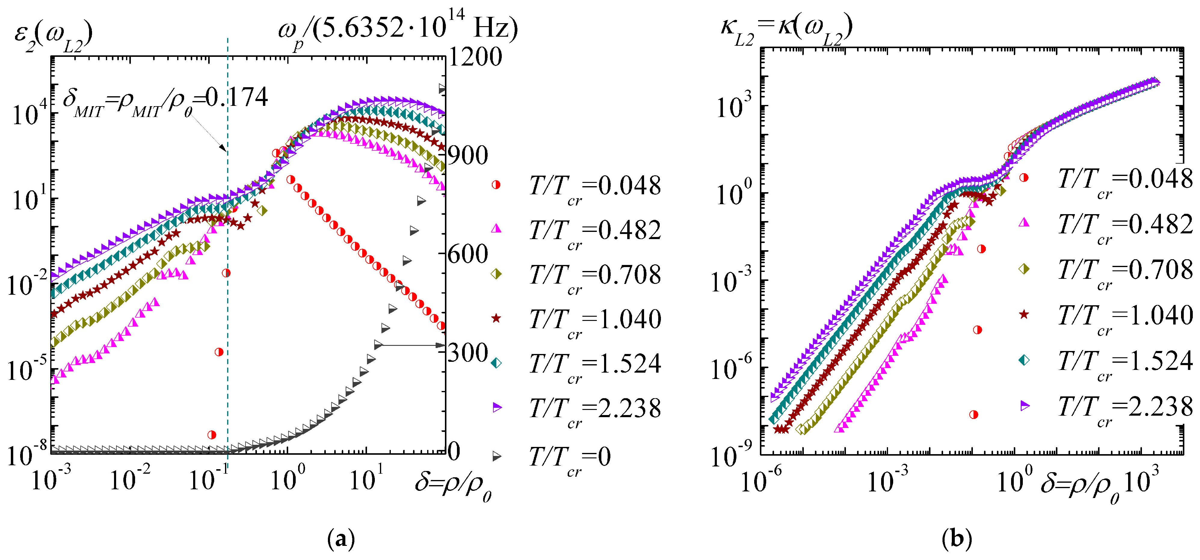
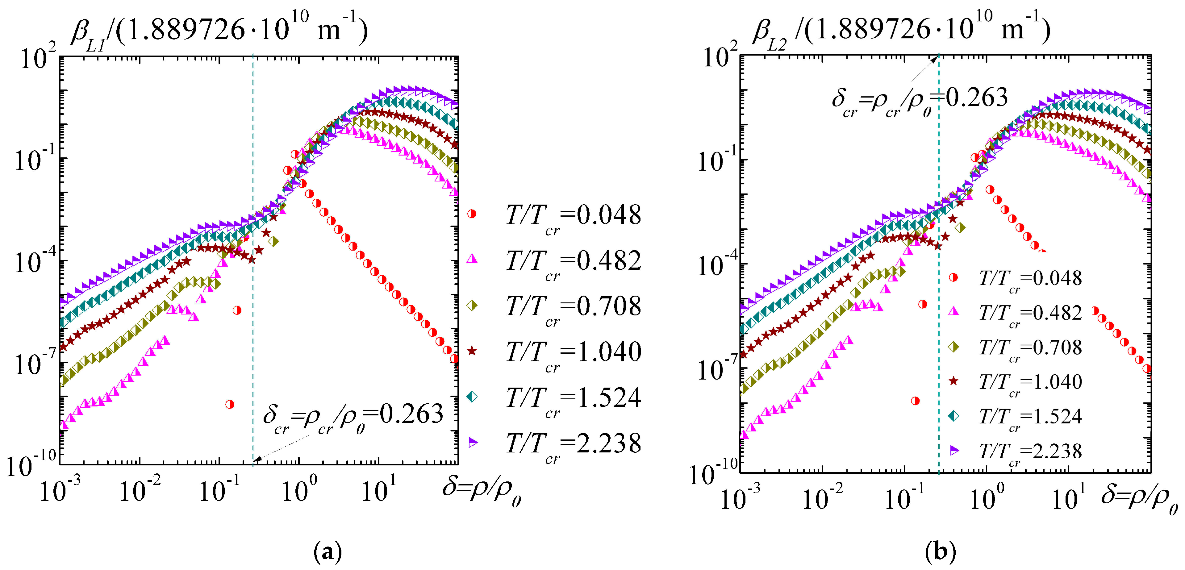
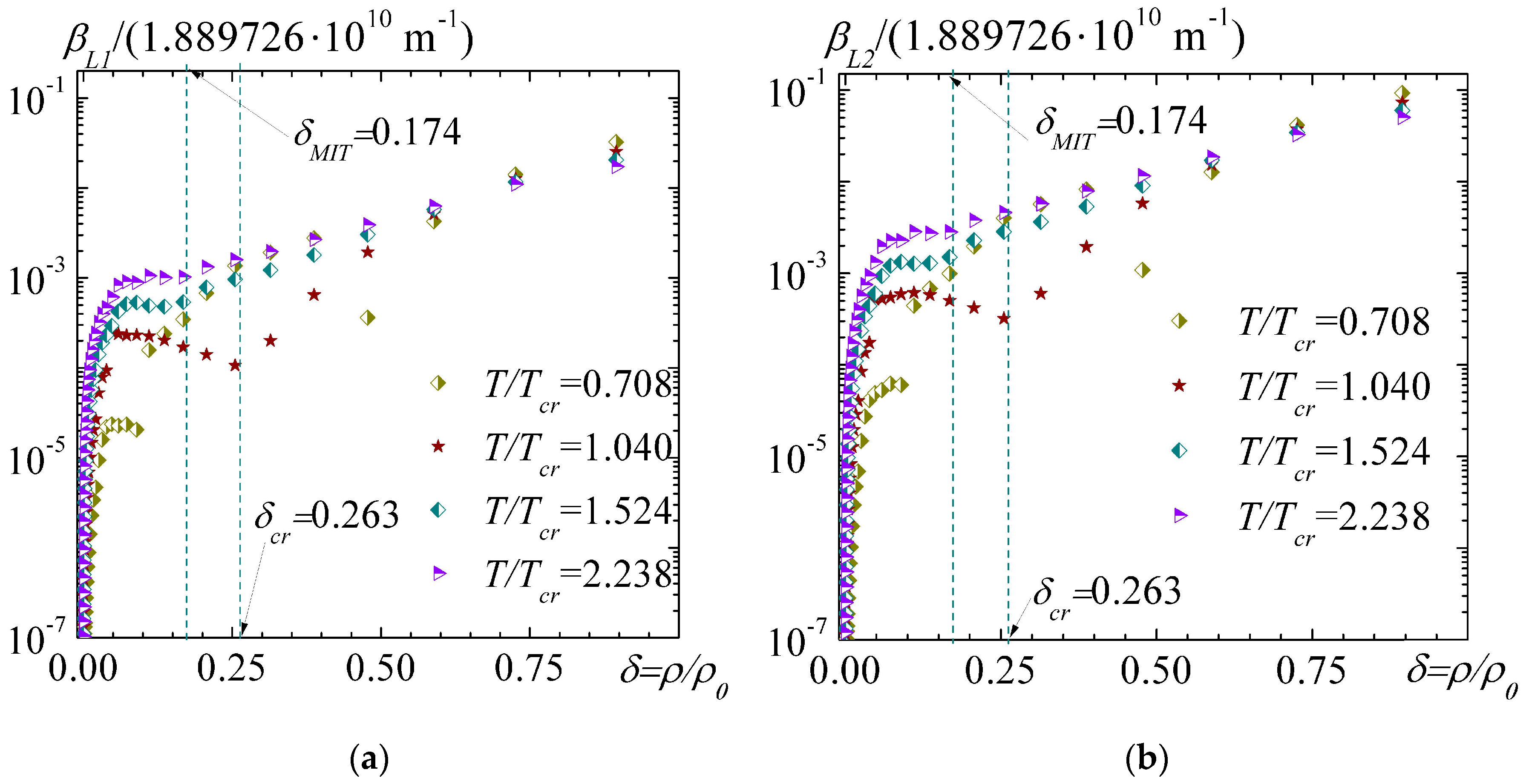
2.2. Optical Properties of Metal Irradiated by Pulsed Radiation from a Solid-State Laser

The electric field of a laser pulse incident along the normal to a metal surface can be expressed as E = E₀(t)exp(−iω₀t), where ω₀ = cλ_L⁻¹ is its frequency, λ_L is the wavelength of the laser radiation, and E₀ is the envelope of the laser pulse amplitude that changes slowly in comparison with its frequency ω₀. We used a pulsed Q-switched Nd:YAG solid-state LOTIS TII LS-2134D laser for the experiments [39,40]. This laser could produce the radiation of the first and second harmonics with wavelengths of λ_L1 = 1064 nm (ω_L1 = 2.82 × 10¹⁴, s⁻¹) and λ_L2 = 532 nm (ω_L2 = 5.64 × 10¹⁴, s⁻¹), respectively. Here and below, the index “L1” means the first harmonic of laser radiation, and “L2” means the second one.

To determine the plasma’s optical characteristics, we assumed that the plasma is uniform and isotropic and that the electric field intensity E(ω) is low.

In this case, the distribution function of electrons can be expressed as f = f₀ + v_e·f₁/v_e = f₀ + p·f₁/p, where v_e·f₁/v_e << f₀ (here, v_e and p are the velocity and momentum). Due to the high laser frequencies, the symmetric function does not explicitly depend on the time since it depends on the temperature and ion concentration. The change in the last ones is determined by the slow hydrodynamic processes. Hence, f₀ = (exp((ε_e − μ₁)/T) + 1)⁻¹ is the equilibrium Fermi–Dirac function we used both in [1] and in the previous section. Then, in the approximation we used for solving the Boltzmann equation, the expression for the asymmetric term of the distribution function of electrons in a periodic electric field takes the following form:

$$f_1(\omega )=-\frac{e{v}_e\frac{\partial f_0}{\partial {\epsilon }_e}}{-i\omega +{\nu }_{ei}({\epsilon }_e)}E(\omega )=\frac{e{\left(\frac{2{\epsilon }_e}{m}\right)}^{1/2}\frac{\partial f_0}{\partial {\mu }_1}}{-i\omega +{(2{\epsilon }_e/m)}^{1/2}{l}_{j,eff}{}^{-1}({\epsilon }_e)}E(\omega )$$

(28)

In (28), l_j,eff(ε_e) is the free path of an electron. The technique used to determine this value was discussed in the previous section as follows:

$$\begin{array}{l}{j}^{\prime }=2e{\displaystyle \int v_{e}f\frac{d^{3}p}{{(2\pi ħ)}^3}}=\frac{{(2m)}^{3/2}{e}^2}{3m{\pi }^2{ħ}^3}\frac{\partial }{\partial {\mu }_1}{\displaystyle {\int }_0^{\infty }\frac{{\epsilon }_e{}^{3/2}{f}_{0}d{\epsilon }_e}{-i\omega +{\nu }_{ei}({\epsilon }_e)}}E=\frac{2z_i{n}_i{e}^2}{3m}\frac{\frac{\partial }{\partial {\mu }_1}{\displaystyle {\int }_0^{\infty }\frac{{\epsilon }_e{}^{3/2}{f}_{0}d{\epsilon }_e}{-i\omega +{\nu }_{ei}({\epsilon }_e)}}}{{\displaystyle {\int }_0^{\infty }{\epsilon }_e{}^{1/2}{f}_{0}d{\epsilon }_e}}E=\\ =\left(\frac{2z_i{n}_i{e}^2}{3m}\frac{\frac{\partial }{\partial {\mu }_1}{\displaystyle {\int }_0^{\infty }\frac{{\nu }_{ei}({\epsilon }_e){\epsilon }_e{}^{3/2}{f}_{0}d{\epsilon }_e}{{\omega }^2+{\nu }_{ei}{}^2({\epsilon }_e)}}}{{\displaystyle {\int }_0^{\infty }{\epsilon }_e{}^{1/2}{f}_{0}d{\epsilon }_e}}+i\omega \frac{2z_i{n}_i{e}^2}{3m}\frac{\frac{\partial }{\partial {\mu }_1}{\displaystyle {\int }_0^{\infty }\frac{{\epsilon }_e{}^{3/2}{f}_{0}d{\epsilon }_e}{{\omega }^2+{\nu }_{ei}{}^2({\epsilon }_e)}}}{{\displaystyle {\int }_0^{\infty }{\epsilon }_e{}^{1/2}{f}_{0}d{\epsilon }_e}}\right)E=\\ =-i\omega \frac{{\epsilon }^{\prime }(\omega )-1}{4\pi }E=-i\omega \frac{{\epsilon }_1(\omega )-1+i{\epsilon }_2(\omega )}{4\pi }E.\end{array}$$

Then, one can obtain the following expressions for the real and imaginary parts of the complex permittivity:

$${\epsilon }_1(\omega )=1-\frac{2{\omega }_p{}^2}{3}\frac{\frac{\partial }{\partial {\mu }_1}{\displaystyle {\int }_0^{\infty }\frac{{\epsilon }_e{}^{3/2}{f}_{0}d{\epsilon }_e}{{\omega }^2+{\nu }_{ei}{}^2({\epsilon }_e)}}}{{\displaystyle {\int }_0^{\infty }{\epsilon }_e{}^{1/2}{f}_{0}d{\epsilon }_e}}=1-\frac{2{\overline{\omega }}_p{}^2}{3}\frac{\frac{\partial }{\partial x}{\displaystyle {\int }_0^{\infty }\frac{{\xi }^{3/2}{f}_0\left(\xi -x\right)d\xi }{{\overline{\omega }}^2+{\overline{\nu }}_{ei}{}^2(\xi )}}}{F_{1/2}\left(x\right)}$$

(29)

$${\epsilon }_2(\omega )=\frac{2{\omega }_p{}^2}{3\omega }\frac{\frac{\partial }{\partial {\mu }_1}{\displaystyle {\int }_0^{\infty }\frac{{\nu }_{ei}({\epsilon }_e){\epsilon }_e{}^{3/2}{f}_{0}d{\epsilon }_e}{{\omega }^2+{\nu }_{ei}{}^2({\epsilon }_e)}}}{{\displaystyle {\int }_0^{\infty }{\epsilon }_e{}^{1/2}{f}_{0}d{\epsilon }_e}}=\frac{2{\overline{\omega }}_p{}^2}{3\overline{\omega }}\frac{\frac{\partial }{\partial x}{\displaystyle {\int }_0^{\infty }\frac{{\overline{\nu }}_{ei}(\xi ){\xi }^{3/2}{f}_0(\xi -x)d\xi }{{\overline{\omega }}^2+{\overline{\nu }}_{ei}{}^2(\xi )}}}{F_{1/2}(x)}$$

(30)

In (29) and (30), ${\omega }_p={(4\pi z_i{n}_i{e}^2/m)}^{1/2}={\omega }_{au}{\overline{\omega }}_p,\hspace{0.17em}\hspace{0.17em}{\overline{\omega }}_p={(4\pi z_i{n}_i{e}^2/m)}^{1/2}{\omega }_{au}{}^{-1}$ is the frequency of plasma oscillations of electrons, and ω_au = E_h/ħ is the basic frequency in the SAU (see Appendix A). The high-frequency ($\overline{\omega }>>{\overline{\nu }}_{ei}$) asymptotic of ${\epsilon }_{1,HF}(\overline{\omega })$ follows from relation (29). It does not depend on the statistics of electrons as follows [25]:

$${\epsilon }_{1,HF}(\omega )=1-\frac{2{\overline{\omega }}_p{}^2}{3{\overline{\omega }}^2}\frac{\frac{\partial }{\partial x}{\displaystyle {\int }_0^{\infty }{\xi }^{3/2}{f}_0\left(\xi -x\right)d\xi }}{F_{1/2}\left(x\right)}=1-\frac{2{\overline{\omega }}_p{}^2}{3{\overline{\omega }}^2}\frac{{F^{\prime }}_{3/2}\left(x\right)}{F_{1/2}\left(x\right)}=1-\frac{2{\overline{\omega }}_p{}^2}{3{\overline{\omega }}^2}\frac{3F_{1/2}\left(x\right)}{2F_{1/2}\left(x\right)}=1-\frac{{\overline{\omega }}_p{}^2}{{\overline{\omega }}^2}$$

Expressions (29) and (30) in an equivalent form for the laser frequency ${\overline{\omega }}_L={\omega }_L/{\omega }_{au}$ will be the following:

$$\begin{array}{l}{\epsilon }_1\left({\overline{\omega }}_L\right)=1-\frac{2{\overline{\omega }}_p{}^2}{3{\overline{\omega }}_L{}^2}\frac{J_{11}(x)-J_{12}(x)}{F_{1/2}(x)},\\ J_{11}(x)={\displaystyle {\int }_0^{\infty }\frac{{\overline{\omega }}_L{}^2{\xi }^{3/2}d\xi }{\left(\exp (\xi -x)+1\right)\left({\overline{\omega }}_L{}^2+{\overline{\nu }}_{ei}{}^2(\xi )\right)}},J_{12}(x)={\displaystyle {\int }_0^{\infty }\frac{{\overline{\omega }}_L{}^2{\xi }^{3/2}d\xi }{{\left(\exp (\xi -x)+1\right)}^2\left({\overline{\omega }}_L{}^2+{\overline{\nu }}_{ei}{}^2(\xi )\right)};}\end{array}$$

(31)

$$\begin{array}{l}{\epsilon }_2\left({\overline{\omega }}_L\right)=\frac{2{\overline{\omega }}_p{}^2}{3{\overline{\omega }}_L{}^2}\frac{J_{21}(x)-J_{22}(x)}{F_{1/2}(x)},\\ J_{21}(x)={\displaystyle {\int }_0^{\infty }\frac{{\overline{\omega }}_L{\overline{\nu }}_{ei}(\xi ){\xi }^{3/2}d\xi }{\left(\exp (\xi -x)+1\right)\left({\overline{\omega }}_L{}^2+{\overline{\nu }}_{ei}{}^2(\xi )\right)}},J_{22}(x)={\displaystyle {\int }_0^{\infty }\frac{{\overline{\omega }}_L{\overline{\nu }}_{ei}(\xi ){\xi }^{3/2}d\xi }{{\left(\exp (\xi -x)+1\right)}^2\left({\overline{\omega }}_L{}^2+{\overline{\nu }}_{ei}{}^2(\xi )\right)}}.\end{array}$$

(32)

To calculate the integrals J₁₁(x), J₁₂(x), J₂₁(x), and J₂₂(x), one can use the method analogous to the one used for the calculation of the kinetic coefficients ${\overline{M}}_{0\beta }$ in the region δ < 1 (see (24)). Then, the expressions for these integrals will be as follows:

$$J_{11}(x)=\{\begin{array}{l}{A}_1{}^2{\displaystyle {\int }_0^{\infty }\frac{{\xi }^{9/2}d\xi }{\left(\exp (\xi -x)+1\right)\left(1+A_1{}^2{\xi }^3\right)},A_1=\frac{S_{ii}{\overline{\omega }}_L{\overline{T}}^{3/2}}{\sqrt{2}\pi {\overline{n}}_i{\Lambda }_j},S_{ii}>0}\\ {\displaystyle {\int }_0^{\infty }\frac{{\xi }^{3/2}d\xi }{\left(\exp (\xi -x)+1\right)\left(1+A_2{}^2\xi \right)},A_2=\frac{\sqrt{2\overline{T}}}{{\overline{\omega }}_L{\overline{r}}_s},S_{ii}\le 0}\end{array},$$

(33)

$$J_{12}(x)=\{\begin{array}{l}{A}_1{}^2{\displaystyle {\int }_0^{\infty }\frac{{\xi }^{9/2}d\xi }{{\left(\exp (\xi -x)+1\right)}^2\left(1+A_1{}^2{\xi }^3\right)},A_1=\frac{S_{ii}{\overline{\omega }}_L{\overline{T}}^{3/2}}{\sqrt{2}\pi {\overline{n}}_i{\Lambda }_j},S_{ii}>0}\\ {\displaystyle {\int }_0^{\infty }\frac{{\xi }^{3/2}d\xi }{{\left(\exp (\xi -x)+1\right)}^2\left(1+A_2{}^2\xi \right)},A_2=\frac{\sqrt{2\overline{T}}}{{\overline{\omega }}_L{\overline{r}}_s},S_{ii}\le 0}\end{array},$$

(34)

$$J_{21}(x)=\{\begin{array}{l}{A}_1{\displaystyle {\int }_0^{\infty }\frac{{\xi }^{3}d\xi }{\left(\exp (\xi -x)+1\right)\left(1+A_1{}^2{\xi }^3\right)},A_1=\frac{S_{ii}{\overline{\omega }}_L{\overline{T}}^{3/2}}{\sqrt{2}\pi {\overline{n}}_i{\Lambda }_j},S_{ii}>0}\\ A_2{\displaystyle {\int }_0^{\infty }\frac{{\xi }^{2}d\xi }{\left(\exp (\xi -x)+1\right)\left(1+A_2{}^2\xi \right)},A_2=\frac{\sqrt{2\overline{T}}}{{\overline{\omega }}_L{\overline{r}}_s},S_{ii}\le 0}\end{array},$$

(35)

$$J_{22}(x)=\{\begin{array}{l}{A}_1{\displaystyle {\int }_0^{\infty }\frac{{\xi }^{3}d\xi }{{\left(\exp (\xi -x)+1\right)}^2\left(1+A_1{}^2{\xi }^3\right)},A_1=\frac{S_{ii}{\overline{\omega }}_L{\overline{T}}^{3/2}}{\sqrt{2}\pi {\overline{n}}_i{\Lambda }_j},S_{ii}>0;}\\ A_2{\displaystyle {\int }_0^{\infty }\frac{{\xi }^{2}d\xi }{{\left(\exp (\xi -x)+1\right)}^2\left(1+A_2{}^2\xi \right)},A_2=\frac{\sqrt{2\overline{T}}}{{\overline{\omega }}_L{\overline{r}}_s},S_{ii}\le 0}.\end{array}$$

(36)

If a laser electromagnetic wave propagates to a dispersive non-magnetic medium, then one can consider it to be a monochromatic plane wave with a complex wavenumber $k_L=\sqrt{{\epsilon }^{\prime }}{\omega }_L/c=(n_L+i{\kappa }_L){\omega }_L/c$ [41]. Here, n_L = n(ω_L) is the refractive index, and κ_L = κ(ω_L) is the absorption coefficient of the medium. If we square the wavenumber, we can obtain the following expressions: n_L² − κ_L² = ε₁(ω_L), 2n_Lκ_L = ε₂(ω_L). Then, the expressions for n_L and κ_L will be as follows:

$$n_L=\sqrt{\frac{{\epsilon }_1+\sqrt{{\epsilon }_1{}^2+{\epsilon }_2{}^2}}{2}},\hspace{0.17em}{\kappa }_L=\sqrt{\frac{-{\epsilon }_1+\sqrt{{\epsilon }_1{}^2+{\epsilon }_2{}^2}}{2}}$$

(37)

The solution of the one-dimensional Helmholtz equation gives the spatial distribution of the envelope of the electric field of the laser pulse as follows:

$$\frac{{\partial }^{2}E(z,{\omega }_L)}{\partial z^2}+\frac{\left(\left(n_L{}^2-{\kappa }_L{}^2\right)+i2n_L{\kappa }_L\right){\omega }_L{}^2}{c^2}E(z,{\omega }_L)=0$$

(38)

The change in the internal energy of the plasma due to laser heating depends at least on the plasma density and temperature. It can be expressed as follows [42,43]:

$$Q_L(t,z)=I_L(t){\beta }_L{\left|E(t,z)/E_L(t)\right|}^2=I_L(t){\beta }_L\exp \left(-{\displaystyle {\int }_z^{\infty }{\beta }_L(z^{\prime })}d{z}^{\prime }\right)$$

(39)

Here, I_L(t) is the laser radiation intensity, and ${\beta }_L=a_B{}^{-1}{\overline{\beta }}_L=a_B{}^{-1}{\epsilon }_2({\overline{\omega }}_L){\overline{\omega }}_L/\overline{c}$ is the dimensional absorption coefficient of the laser radiation, with the dimension m⁻¹ in SI. Expressions (31)–(36) and (39) make it possible to calculate all the optical characteristics of the metal in a broad range of densities and temperatures.

The obtained data presented in Figure 7, Figure 8, Figure 9, Figure 10 and Figure 11 allow one to conclude that plasma is transparent for optical radiation at a low density and weak ionization. Thus, for T/T_cr = 0.048, the real part of the permittivity becomes negative when passing from δ = 0.168 to δ = 0.207. It indicates the quasi-free conduction electrons’ appearance (see Figure 7a and Figure 9a). The density value of δ_MIT = 0.174 corresponding to the metal–insulator PT at T = 0, i.e., the localization of electrons, was calculated using the LmtART ver. 7 software (https://savrasov.physics.ucdavis.edu) [9,10].

The greatest absorption is observed in the region of the compressed state of the metal. One can see it in Figure 8b, Figure 10b and Figure 11. The maximum change in the transport and optical properties of iron is observed near the liquid–gas PT in the area of critical density and in the area of density corresponding to the metal–insulator PT at T = 0.

3. Discussion

Figure 12 demonstrates the behavior of the calculated electrical conductivity of iron as a function of temperature (Figure 12a) and density (Figure 12b).

The dependences of the dimensionless absorption coefficient on the matter density for the first and second laser radiation harmonics are shown in Figure 13.

The change in the electrical conductivity character from a metallic type to a non-metallic one in the range of relative volume V/V₀ = 3–5 (relative density δ = 0.2–0.33) for pressures P = 20–25 kbar was shown in recently published experimental investigations [37,38]. According to these papers, the presence of a metal–insulator PT is shown to be near the critical point of the liquid–gas PT, which was predicted in [44]. Thus, it seems reasonable to compare our results with the experimental data of these papers. It should be taken into account that the estimates of the critical parameters of iron used in [37,38] to interpret these experiments were the following: ρ_cr = 2.03 g/cm³, T_cr = 9600 K, and P_cr = 8.25 kbar [45]. But we will use the following parameters of the critical point of iron, which we obtained from [1]: ρ_cr = 2.07 g/cm³, T_cr = 10867 K, and P_cr = 12.56 kbar. The experimental pressure range of P = 20–25 kbar corresponds to P_exp/P_cr = 2.424–3.03 in [37,38] and P_exp/P_cr = 1.59–1.99 in our paper [1]. The change in the electrical conductivity character was observed experimentally in the range V/V₀ = 3–5. This range in Figure 12a corresponds to three isodensities (isochores): (1) δ = 0.21 (V/V₀ = 4.84), (2) δ = 0.26 (V/V₀ = 3.92), and (3) δ = 0.31 (V/V₀ = 3.18). The first value corresponds to the change in resistivity: T/T_cr = 0.71 ρ_e = 29.03 μΩ·m, T/T_c = 1.04 ρ_e = 141.77 μΩ·m, T/T_c = 1.52 ρ_e = 24.96 μΩ·m. The second value corresponds to T/T_c = 0.71 ρ_e = 14.51 μΩ·m, T/T_c = 1.04 ρ_e = 186.89 μΩ·m, T/T_c = 1.52 ρ_e = 20.57 μΩ·m. The third value corresponds to T/T_c = 0.71 ρ_e = 10.33 μΩ·m, T/T_c = 1.04 ρ_e = 99.38 μΩ·m, T/T_c = 1.52 ρ_e = 16.21 μΩ·m. These results agree with the data shown in Figure 12b and Figure 13a,b. The last two figures show that at δ = 0.263 (V/V₀ = 3.802), the absorption coefficient of the laser radiation energy decreases sharply. This behavior of the resistivity and energy absorption coefficient of laser radiation in the near-critical region of the liquid–gas PT is explained by the behavior of the structural factor S_ii = K_ii/n_iT, which is responsible for the density fluctuations in the near-critical and supercritical areas (see Figure 2a, as well as [46]). It should be noted that the curves in Figure 12a, corresponding to the density below the PT at T = 0 (δ = 0.110–0.168), demonstrate the plasma behavior with the increasing temperature. The curves corresponding to the density range δ = 0.726–1.103 show a uniform change in the electrical conductivity from a metallic character to a plasma one with a temperature increase.

4. Conclusions

In Section 2.1, on the example of iron, the expressions of the following transport properties of a matter in the expanded and compressed state were obtained: electrical conductivity σ(ρ,T), electronic thermal conductivity κ(ρ,T), and thermoelectric coefficient α(ρ,T). These expressions were used to calculate the above-mentioned parameters in a broad range of densities and temperatures. In Section 2.2, the expressions for the real and imaginary parts of the permittivity and the absorption coefficient laser radiation were obtained. The analysis of these characteristics in the expanded and compressed states was carried out. They appear to be consistent with the known results in limiting cases.

The impurity additions to an ordered medium are widely used for theoretical studies of the metal–insulator PT. These impurities violate the original order [7,47,48,49,50]. Then, we can consider two limiting cases. The first case corresponds to the white noise when the correlation radius between the impurities is zero. The second corresponds impurity to the infinite correlation radius [7]. The case of S_ii(δ,T) = 1 corresponds to the first limiting case of uncorrelated impurities in the commonly developed theoretical models of the metal–insulator PT. The process descriptions we use in the near-critical region, S_ii(δ,T) ≠ 1 and δ < 1, are closer to the second limiting case, supposing an infinite correlation radius. Therefore, the properties and structural PTs of metals in the expanded and compressed states are the aims of further studies.

Thus, it was established that the behaviors of the transport and optical characteristics in the near-critical and supercritical regions of iron in the liquid state do not contradict the experimental data [37,38], and the proposed model can be applied to the estimation of metal properties in compressed and expanded states under the influence of high-density energy fluxes.

References

1. Volkov, N.B.; Lipchak, A.I. Thermodynamic functions of a metal exposed to high energy densities in composed and expanded states. Condens. Matter 2022, 7, 61. [Google Scholar] [CrossRef]
2. Maxwell, J.C. On the Dynamical Theory of Gases. In Scientific Papers of James Clark Maxwell, 2nd ed.; Two Volumes Bound As One; Niven, W.D., Ed.; Dover Publications, Inc.: Mineola, NY, USA, 1965; Volume 2, pp. 26–78. [Google Scholar]
3. Boltzmann, L. Lectures on Gas Theory; Stephen, G. Brush, S.G., Translator; Dover Publications, Inc.: Mineola, NY, USA, 1995. [Google Scholar]
4. Lorentz, H.A. The Theory of Electrons: Its Applications to the Phenomena of Light and Radiant Heat (Dover Books on Physics), 2nd ed.; Dover Publications, Inc.: Mineola, NY, USA, 2011. [Google Scholar]
5. Abrikosov, A.A.; Gorkov, L.P.; Dzyaloshinskii, I.E. Methods of Quantum Field Theory in Statistical Physics; Pergamon Press Ltd.: Oxford, UK, 1963. [Google Scholar]
6. Mahan, G.D. Many-Particle Physics, 3rd ed.; Kluwer Academic/Plenum Publishers: New York, NY, USA, 2000. [Google Scholar]
7. Sadovskii, M.V. Diagrammatics: Lectures on Selected Problems in Condensed Matter Theory; World Scientific Publishing Co. Pte. LTD: Singapore, 2006. [Google Scholar]
8. Mahan, G.D. Quantum transport equation for electric and magnetic fields. Phys. Rep. 1987, 145, 251–318. [Google Scholar] [CrossRef]
9. Savrasov, S.Y. Linear-response theory and lattice dynamics: A muffin-orbital approach. Phys. Rev. B 1996, 54, 16470–16486. [Google Scholar] [CrossRef] [PubMed] [Green Version]
10. Savrasov, S.Y.; Savrasov, D.Y. Electron-phonon interactions and related physical properties of metals from linear-response theory. Phys. Rev. B 1996, 54, 16487–16501. [Google Scholar] [CrossRef] [PubMed] [Green Version]
11. Maksimov, E.G.; Savrasov, D.Y.; Savrasov, S.Y. The electron–phonon interaction and the physical properties of metals. Physics-Uspekhi 1997, 40, 337–358. [Google Scholar] [CrossRef]
12. Giustino, F. Electron–phonon interactions from first principles. Rev. Mod. Phys. 2017, 89, 015003. [Google Scholar] [CrossRef] [Green Version]
13. Ichimaru, S. Strongly coupled plasmas: High-density classical plasmas and degenerate electron liquids. Rev. Mod. Phys. 1982, 54, 1017–1059. [Google Scholar] [CrossRef]
14. Kraeft, W.-D.; Kremp, D.; Ebeling, W.; Roepke, G. Quantum Statistics of Charged Particle Systems; Akademy-Verlag: Berlin, Germany, 1986. [Google Scholar]
15. Ebeling, W.; Foerster, A.; Fortov, V.E.; Gryaznov, V.K.; Polishchuk, A.Y. Thermophysical Properties of Hot Dense Plasmas; B.G. Teubner Verlagsgeselschaft: Stuttgart, Germany, 1991. [Google Scholar]
16. Ebeling, W.; Fortov, V.E.; Filinov, V.S. Quantum Statistics of Dense Gases and Nonideal Plasmas; Springer Int. Publishing AG: Berlin/Heidelberg, Germany, 2017. [Google Scholar]
17. Fortov, V.E.; Filinov, V.S.; Larkin, A.S.; Ebeling, W. Statistical Physics of Dense Gases and Nonideal Plasmas; Fizmatlit: Moscow, Russia, 2020. [Google Scholar]
18. Povarnitsyn, M.E.; Knyazev, D.V.; Levashov, P.R. Ab initio simulation of complex dielectric function for dense aluminum plasma. Contrib. Plasma Phys. 2012, 52, 145–148. [Google Scholar] [CrossRef] [Green Version]
19. Knyazev, D.V.; Levashov, P.R. Ab initio calculation of transport and optical properties of aluminum: Influence of simulation parameters. Comput. Mater. Sci. 2013, 79, 817–829. [Google Scholar] [CrossRef]
20. Knyazev, D.V.; Levashov, P.R. Transport and optical properties of warm dense aluminum in two-temperature regime: Ab initio calculation and semi-empirical approximation. Phys. Plasmas 2014, 21, 073302. [Google Scholar] [CrossRef]
21. Volkov, N.B.; Chingina, E.A.; Yalovets, A.P. Dynamical equations and transport coefficients for the metals at high pulse electromagnetic fields. J. Phys. Conf. Ser. 2016, 774, 012147. [Google Scholar] [CrossRef]
22. Volkov, N.B.; Nemirovsky, A.Z. The ionic composition of the non-ideal plasma produced by a metallic sphere isothermally expanding into vacuum. J. Phys. D Appl. Phys. 1991, 24, 693–701. [Google Scholar] [CrossRef]
23. Shabanskii, V.P. Transfer processes in conductors with regard to nonlinear effects. Sov. Phys. JETP 1957, 4, 497–508. [Google Scholar]
24. Volkov, N.B. Nonlinear Dynamics of Current-Carrying Plasma-Like Media. Habilitation Thesis, Institute of Electrophysics UB RAS, Ekaterinburg, Russia, 1999. [Google Scholar]
25. Ginzburg, V.L. The Propagation of Electromagnetic Waves in Plasmas, 2nd ed.; Pergamon Press LTD: Oxford, UK, 1970. [Google Scholar]
26. Volkov, N.B. A plasma model of the conductivity of metals. Zhurnal Tekhnicheskoj Fiz. 1979, 49, 2000–2002. [Google Scholar]
27. Landau, L.D.; Lifshitz, E.M. Statistical Physics, Part 1. In Course of Theoretical Physics, 3rd ed.; Pergamon Press LTD: Oxford, UK, 1980; Volume 5. [Google Scholar]
28. Lifshitz, E.M.; Pitaevskii, L.P. Physical Kinetics. In Landau and Lifshitz: Course of Theoretical Physics; Pergamon Press LTD.: Oxford, UK, 1981; Volume 10. [Google Scholar]
29. Martienssen, W.; Warlimont, H. (Eds.) Springer Handbook of Condensed Matter and Materials Data; Springer: Berlin/ Heidelberg, Germany, 2005. [Google Scholar]
30. Ziman, J.M. Principles of the Theory of Solids, 2nd ed.; Cambridge University Press: London, UK, 1972. [Google Scholar]
31. Berman, R. Thermal Conduction in Solids, 2nd ed.; Oxford University Press: Oxford, UK, 1980. [Google Scholar]
32. Harrison, W.A. Pseudopotentials in the Theory of Metals; W. A. Benjamin, INC: New York, NY, USA, 1966. [Google Scholar]
33. Frenkel, J.I. Wave Mechanics: Elementary Theory, 2nd ed.; Dover Publications, INC: Mineola, NY, USA, 1950; Chapter 6. [Google Scholar]
34. Radtsig, A.A.; Smirnov, B.M. Reference Book on Atomic and Molecular Physics; Atomizdat: Moscow, Russia, 1980. [Google Scholar]
35. Kittel, C. Introduction to Solid State Physics, 8th ed.; John Wiley and Sons, Inc.: New York, NY, USA, 2005. [Google Scholar]
36. Chapman, S.; Cowling, T.G. The Mathematical Theory of Non-Uniform Gases, 3rd ed.; Cambridge University Press: Cambridge, UK, 1991. [Google Scholar]
37. Landau, L.D.; Lifshitz, E.M. Electrodynamics of Continuous Media. In Course of Theoretical Physics, 2nd ed.; Pergamon Press LTD: Oxford, UK, 1984; Volume 8. [Google Scholar]
38. Afanasiev, Y.V.; Krokhin, O.N. High-temperature and plasma phenomena arising from the interaction of high-power laser radiation with matter. In Physics of High Energy Densities; International School of Physics “Enrico Fermi” Course, 48; Caldirola, P., Knoepfel, H., Eds.; Academic Press: New York, NY, USA, 1971; Chapter 10. [Google Scholar]
39. Hora, H. Physics of Laser Driven Plasma; John Wiley and Sons, Inc.: New York, NY, USA, 1981. [Google Scholar]
40. Korobenko, V.N.; Rakhel, A.D. Transition of expanded liquid iron to the nonmetallic state under supercritical pressure. J. Exp. Theor. Phys. 2011, 112, 649–655. [Google Scholar] [CrossRef]
41. Korobenko, V.N.; Rakhel, A.D. Observation of a first-order metal-to-nonmetal phase transition in fluid iron. Phys. Rev. B 2012, 85, 014208. [Google Scholar] [CrossRef] [Green Version]
42. Lipchak, A.I.; Barakhvostov, S.V. An investigation of the stability of turning a high-current pulse accelerator on with an optical control. Instrum. Exp. Tech. 2021, 64, 376–380. [Google Scholar] [CrossRef]
43. Lipchak, A.I.; Barakhvostov, S.V.; Volkov, N.B.; Chingina, E.A.; Turmyshev, I.S. The study of instabilities role of plasma in the high-voltage discharge formation initiated by optical radiation at high pressures in high-voltage optical triggered switches. J. Phys. Conf. Series 2021, 2064, 012098. [Google Scholar] [CrossRef]
44. Zeldovich, Y.B.; Landau, L.D. On the relationship between the liquid and gaseous states of metals. Zh. Exp. Teor. Fiz. 1944, 14, 32. [Google Scholar]
45. Fortov, V.E.; Iakubov, I.T. Non-Ideal Plasma; Pergamon Press LTD: New York, NY, USA, 2000. [Google Scholar]
46. Brazhkin, V.V. Phase transformations in liquids and the liquid-gas transition in fluids at supercritical pressures. Phys.-Uspekhi 2017, 60, 954–957. [Google Scholar] [CrossRef]
47. Mott, N.V. Metal-Insulator Transitions; Taylor and Fransis Ltd.: London, UK, 1974. [Google Scholar]
48. Ziman, J.M. Models of Disorder; Cambridge University Press: Cambridge, UK, 1979. [Google Scholar]
49. Lifshits, I.M.; Gredeskul, S.A.; Pastur, L.A. Introduction to the Theory of Disorder Systems; John Wiley and Sons, Inc.: New York, NY, USA, 1988. [Google Scholar]
50. Gantmakher, V.F. Electrons and Disorder in Solids. In International Series of Monographs on Physics; Oxford University Press: Oxford, UK, 2005; Volume 130. [Google Scholar]
Figure 1. The squared Debye wavenumbers (a) and the squared shielding radius of inner electrons (b).
Condensedmatter 08 00070 g001
Figure 2. The long-wavelength structure factor of iron for low (a) and high temperatures (b).
Condensedmatter 08 00070 g002
Figure 3. The electron conductivity (a) and number of electrons in an atomic cell (b) of iron.
Condensedmatter 08 00070 g003
Figure 4. The dependence of iron thermal conductivity (a) and Wiedemann–Franz ratio (b) on density.
Condensedmatter 08 00070 g004
Figure 5. The dependence of iron thermal conductivity (a) and Wiedemann–Franz ratio (b) on temperature.
Condensedmatter 08 00070 g005
Figure 6. The dependence of thermoelectric coefficient on density (a) and temperature (b).
Condensedmatter 08 00070 g006
Figure 7. The real permittivity (a) and refraction index (b) of iron for the first harmonic of laser radiation.
Condensedmatter 08 00070 g007
Figure 8. The imaginary permittivity (a) and absorption factor (b) of iron for the first harmonic of laser radiation.
Condensedmatter 08 00070 g008
Figure 9. The real permittivity (a) and refraction index (b) of iron for the second harmonic of laser radiation.
Condensedmatter 08 00070 g009
Figure 10. The imaginary permittivity (a) and absorption factor (b) of iron for the second harmonic of laser radiation.
Condensedmatter 08 00070 g010
Figure 11. The absorption coefficient of iron for the first (a) and the second (b) harmonics of laser radiation.
Condensedmatter 08 00070 g011
Figure 12. The dependence of electronic conductivity of iron on temperature (a) and density (b).
Condensedmatter 08 00070 g012
Figure 13. The dimensionless iron absorption coefficient for the first (a) and second (b) harmonics of the laser radiation.
Condensedmatter 08 00070 g013
Disclaimer/Publisher’s Note: The statements, opinions and data contained in all publications are solely those of the individual author(s) and contributor(s) and not of MDPI and/or the editor(s). MDPI and/or the editor(s) disclaim responsibility for any injury to people or property resulting from any ideas, methods, instructions or products referred to in the content.