Article

Dispersion in Single-Wall Carbon Nanotube Film: An Application of Bogoliubov–Valatin Transformation for Hamiltonian Diagonalization

by
Chandra M. Adhikari
1,*,
Da’Shawn M. Morris
1,
Thomas W. Noonan
1,
Tikaram Neupane
2,
Basu R. Lamichhane
3 and
Bhoj R. Gautam
1
1
Department of Chemistry, Physics and Materials Science, Fayetteville State University, Fayetteville, NC 28301, USA
2
Department of Chemistry and Physics, The University of North Carolina at Pembroke, Pembroke, NC 28372, USA
3
Natural Sciences Collegium, Eckerd College, St. Petersburg, FL 33711, USA
*
Author to whom correspondence should be addressed.
Condens. Matter 2023, 8(2), 53; https://doi.org/10.3390/condmat8020053
Submission received: 4 May 2023 / Revised: 8 June 2023 / Accepted: 13 June 2023 / Published: 16 June 2023
(This article belongs to the Section Condensed Matter Theory)

Abstract

:
We present a theoretical study on the energy dispersion of an ultrathin film of periodically-aligned single-walled carbon nanotubes (SWCNTs) with the help of the Bogoliubov–Valatin transformation. The Hamiltonian of the film was derived using the many-particle green function technique in the Matsubara frequency formalism. The periodic array of SWCNTs was embedded in a dielectric with comparatively higher permittivity than the substrate and the superstrate such that the SWCNT film became independent with the axis of quantization but keeps the thickness as the variable parameter, making the film neither two-dimensional nor three-dimensional, but transdimensional. It was revealed that the energy dispersion of the SWCNT film is thickness dependent.

1. Introduction

A cylindrically rolled-up hexagonal two-dimensional (2D) lattice of carbon, called a single-walled carbon nanotube (SWCNT), exhibits 2D-lattice-rolling axis-dependent conductive behavior, providing a remarkable possibility for use in the electronics industry. Carbon nanotubes (CNTs) have a low density, as low as 1.3 g/cm 3 [1], but a tensile strength as high as 100 gigapascals (GPa) [2], making them materials with a high specific strength up to nearly 300 times of high-carbon steel’s specific strength. In a 2D hexagonal sheet of carbon called graphene, a vector connecting any two carbon atoms can be expressed in terms of two linearly-independent vectors, u and v , as n u + m v , where n and m are integers and the pair ( n , m ) is called its chirality. Chirality specifies how the graphene sheet is rolled up to form an SWCNT. The SWCNTs with n m = 0 are metallic and have an electric current density of about 10 3 times more than that of copper [3]. SWCNTs with n m = 3 , where is an integer, are quasi-metallic, while the other SWCNTs are semiconducting, effectively affirming that the electrical conductivity of SWCNTs is chirality-dependent [4,5]. SWCNTs also show promising thermal conductivity along the axis of SWCNT [6] and optical properties such as photoluminescence [7], hyperbolic metamaterial [8], and charge transporting layers for perovskite solar cells [9].
We considered an SWCNT film of a homogeneous array of infinitely thin, periodically aligned, identical SWCNTs oriented along the y-axis, as shown in Figure 1. The film was embedded in a medium of effective relative permittivity ϵ , and sandwiched in between a substrate and a superstrate of relative permittivities ϵ 1 and ϵ 2 , respectively, to form a reactangular thin-film. Carbon nanotubes have a circular cross-section radius R = a 0 / π n 2 + m n + m 2 , where ( n , m ) represents the chiral vector for ( n , m ) SWCNT and a 0 = 3 b / 2 , where b = 0.142 nm is the carbon–carbon interatomic distance in an SWCNT. If e and e are two charges in the n th and th SWCNT cylinders with uniform charge distribution, the Coulomb interaction between these charges can be approximated by the Coulomb interaction between two uniformly charged rings whose radius is the same as that of the respective cylinders [10,11]. An interesting thing happens as ϵ 1 + ϵ 2 ϵ and d ρ , where d is the thickness of the dielectric in which the SWCNTs are immersed, and ρ is the distance between the rings of the unit cells of the n th and th SWCNTs. The Coulomb interaction between the rings of unit cells loses the dependence on its vertical component (for the geometry we choose, it is the z-component) but still retains the thickness of the film as a parameter to represent the vertical size of the system and behaves as a stronger Keldysh–Rytova (KR) interaction [12]. This brings the system into the transdimensional (TD) regime [13]. TD materials are quite interesting, as their optical and electronic properties show comparatively stronger dependences on structural parameters such as thickness, stoichiometry, doping, strain, and surface termination than respective 3 D -bulk material properties and extreme sensitivity to external optical and electrical stimuli such as 2 D -counterparts [14].
The mathematical formulation is quite involved, as it requires setting the Hamiltonian for an array of interacting SWCNTs with the help of many-body Green’s function technique in the so-called Matsubara formulation [15] and diagonalizing it to find the eigenvalues. The purpose of the paper is two-fold: first, to investigate the energy dispersion in the film of SWCNTs along with its dependency on the film thickness and second, to explore the diagonalization technique, such as the Bogoliubov–Valatin transformation [16,17,18], for a matrix whose entries are complex mathematical functions. The energy dispersion in the thin SWCNT films neither varies with the square of momentum like that of a 3 D bulk, i.e., E ( q ) q 2 [19], nor it is linear with the absolute value of the momentum as in the case of a 2 D graphene sheet from which it is made, i.e., E ( q ) q (see Ref. [20]). The energy variation with momentum has a complicated mathematical expression.
A non-singular square matrix of order n can be diagonalized if and only if it has n linearly independent eigenvectors, corresponding to the eigenvalues of the matrix [21]. Similarity transformation is one of the most common techniques of diagonalizing a matrix. A square matrix S can be diagonalized this way with the help of an invertible matrix, P, calculating a matrix S using S = P 1 S P , where S is similar to S and such a transformation is a similar transformation. In this process, a non-diagonal square matrix S is transformed to a diagonal square matrix S of the same order, such that the eigenvalues of the matrices S and S will be the same. Dimension reduction is often a preliminary step in the diagonalization of a higher dimensional square matrix, which can also be achieved using the adjacency graph technique [22,23] in addition to the Hamiltonian and momentum conservations [24,25,26]. Complications arise if matrix elements are mathematical quantities more complex than just numbers or variables. Especially when the Hamiltonian matrix is in a quadratic form of the second quantized creation and annihilation operators, the Bogoliubov–Valatin transformation can be a great tool for diagonalizing the Hamiltonian matrix and obtaining eigenenergies.
The energy dispersion also evaluates the energy band gap of the system. The literature is rich in experimental studies on exciton dynamics and the electronic properties of an isolated SWCNT [27,28,29,30]. The authors reported electronic and excitonic band gaps of various isolated SWCNTs. However, to the best of our knowledge, no excitonic gap for a film of (11,0) SWCNTs has been reported experimentally. The presented model involves resolving the polarization of each SWCNT into its parallel and perpendicular components and evaluating the collective polarization of the film. Polarization-resolved spectroscopy can be used to analyze the film’s dispersion experimentally [31].
This paper is organized as follows. In Section 2, we revisit the Hamiltonian of the SWCNT film of periodically aligned identical SWCNTs in terms of Bose creation and annihilation operators. Next, we devote Section 3 to the diagonalization of the Hamiltonian matrix and energy dispersion for the SWCNT film. We present a numerical example of the dispersion relation by taking an example of a thin film made up of homogeneous, periodically-aligned zigzag (11,0) SWCNTs in Section 4. Conclusions are drawn in Section 5. Gaussian units are used throughout the paper unless otherwise stated.

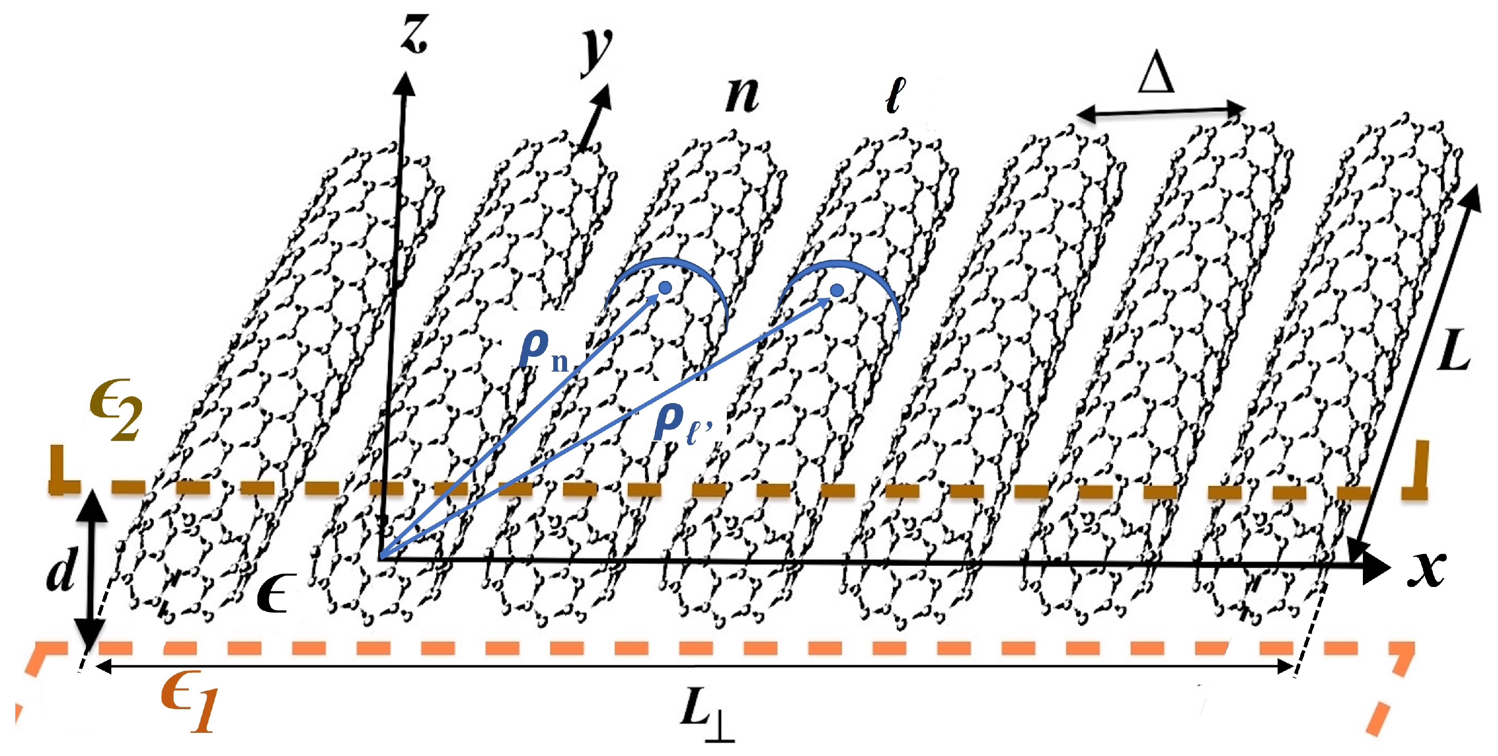
2. Mathematical Formulation

Absorption of a photon in the valence band of an SWCNT excites an electron to the conduction band, leaving a vacant space called a hole in the valance band, thereby creating an exciton. Consequently, the SWCNT becomes polarized, producing an induced dipole moment along the CNT axis. The SWCNTs communicate with each other via dipole–dipole interaction. Due to the depolarization effect, the net polarization along the axis perpendicular to the SWCT alignment is negligible and can be ignored [32,33]. As a result, the net polarization of SWCNT film becomes anisotropic.
The wave vector k , in the xy plane, can be resolved into two components, namely, q and k , which are, respectively, parallel and perpendicular to the direction in which cylinders are aligned, i.e., k = q + k . It is then evident that k = k = q 2 + k 2 , where k = 2 π n x / L . Here, n x takes either one of 0 , ± 1 , ± 2 , , ± N / 2 , where N stands for the total number of SWCNTs. The total Hamiltonian of the system in the wave-vector space can be written as the sum of the unperturbed Hamiltonian of the system, H 0 = q , E ω E b q , E b q , E , and the perturbation H ^ int due to the interaction between different excitations, E and E [10]
H = q , E ω E b q , E b q , E + 1 a Δ q E E V E E ( q ) b q , E b q , E + b q , E b q , E + b q , E b q , E + b q , E b q , E ,
where a and Δ are the translational period along the axis of the SWCNTs and the intertube center-to-center distance in the array of the SWCNTs, respectively. The quantity Δ satisfies Δ 2 R and determines the sparseness of SWCNT in the film. ω E is the excitation energy for an excitation E. The same for the E excitation reads ω E . One can evaluate the total excitation energy as the sum of an internal state exciton energy E exc and the kinetic energy T ( q ) of the exciton due to its longitudinal translational motion,
ω E = E exc + T ( q ) = E exc + 2 q 2 2 M ex ,
where M ex is the effective mass of an exciton. b q , E and b q , E in Equation (1) are well known creation and annihilation operators, which, respectively, creates and annihilates an exciton with longitudinal momentum q and excitation E. The operator b q , E follows the standard commutation relation of Bose–Einstein statistics and satisfies the following identities:
b q , E , b q , E = δ q q δ E E , b q , E , b q , E = b q , E , b q , E = 0 .
The interaction potential V E E ( q ) between different excitations E and E is given by
V E E ( q ) = m * ω p 2 ( 0 , q ) N 2 D X ( E ) T y y ( 0 , q ) X ( E ) ,
where N 2 D is the surface electron density, m * is the electron effective mass, and X ( E ) is the transition dipole associated with an excitation E. T y y ( 0 , q ) = T y y ( k = 0 , q ) is a traceless second rank tensor, which depicts the Fourier transform of the dipole–dipole interaction and plays a role in interrelating excitations in the momentum space. ω p ( 0 , q ) is the SWCNT-plasmon frequency and it can be expressed in terms of zeroth order Bessel functions I 0 ( q R ) and K 0 ( q R ) as [10]
ω p ( 0 , q ) = 4 π e 2 N 2 D ϵ m * d 2 q R I 0 ( q R ) K 0 ( q R ) 1 + ϵ 1 + ϵ 2 / ( q ϵ d ) .
It is evident from Equation (5) that the SWCNT-plasmon frequency is thickness-dependent. For a thick SWCNT film with ϵ 1 + ϵ 2 q ϵ d , the plasmon frequency varies as q , i.e., ω p ( 0 , q ) q , whereas for an ultrathin SWCNT film with ϵ 1 + ϵ 2 q ϵ d , the SWCNT plasmon-frequency is linear with q, i.e., ω p ( 0 , q ) q . The I 0 ( q R ) and K 0 ( q R ) Bessel functions in the SWCNT-plasmon frequency ω p ( 0 , q ) are simply because of the SWCNT’s cylindrical geometry.

3. Bogoliubov–Valatin Transformation Technique of Hamiltonian Diagonalization

We concentrated on the diagonalization of the Hamiltonian (1) using Bogoliubov’s canonical transformation technique [16,17,18] to obtain the dispersion relation associated with the exciton-plasmon excitations in the SWCNT film initiated by illuminating the film with a photon. Consider that u μ ( q , E ) and v μ ( q , E ) are the eigenfunctions of the system with eigenvalues E μ = ω μ such that the system satisfies the following set of equations:
E μ u μ ( q , E ) = E ω E u μ ( q , E ) + q E E V E E ( q ) a Δ v μ ( q , E ) , E μ v μ ( q , E ) = E ω E v μ ( q , E ) + q E E V E E ( q ) a Δ u μ ( q , E ) .
The transformation matrix U for excitons reads
U = u μ ( q , E ) v μ ( q , E ) v μ * ( q , E ) u μ ( q , E ) ,
such that u μ ( q , E ) 2 v μ ( q , E ) 2 = 1 , for which the functions u μ ( q , E ) and v μ ( q , E ) satisfy the following orthogonality and normalization conditions:
u μ ( q , E ) u μ * ( q , E ) v μ ( q , E ) v μ * ( q , E ) = δ μ μ δ q q δ E E , v μ ( q , E ) u μ * ( q , E ) u μ ( q , E ) v μ * ( q , E ) = 0 .
To diagonalize the Hamiltonian (1), we make the Bogoliubov’s canonical transformation of the bosonic operators, as follows:
b q , E = μ u μ ( q , E ) ξ ^ μ ( q ) + v μ ( q , E ) ξ ^ μ ( q ) ,
such that the Hamiltonian (1) can be expressed as
H ^ ( q ) = μ ω μ ( q ) ξ ^ μ ( q ) ξ ^ μ ( q ) ,
where ξ μ ( q ) and ξ μ ( q ) are the new bosonic creation and annihilation operators of exciton-photon excitations at the μ branch on the CNT film. We have here shifted the SWCNT array’s energy in vacuum E vac = H ^ ( q ) μ ω μ ( q ) ξ ^ μ ( q ) ξ ^ μ ( q ) to the origin. Similar to the transformation presented in Equation (9), bosonic operators b q , E , b q , E and b q , E can be expressed in terms of ξ ^ μ ( q ) and ξ ^ μ ( q ) as
b q , E = μ u μ * ( q , E ) ξ ^ μ ( q ) + v μ * ( q , E ) ξ ^ μ ( q ) ,
b q , E = μ u μ ( q , E ) ξ ^ μ ( q ) + v μ ( q , E ) ξ ^ μ ( q ) .
The q argument of the u and v transformation functions for b q , E and b q , E is an absolute value of q because u and v are probability amplitudes. Otherwise, it would mean that the probability amplitudes depend on the propagation direction of the exciton, which is physically invalid. The canonically-transformed ξ ^ μ ( q ) operator can be expressed in terms of b q , E and b q , E operators as
ξ ^ μ ( q ) = q E u μ * ( q , E ) b q , E v μ ( q , E ) b q , E .
The bosonic operators ξ ^ μ ( q ) and ξ ^ μ ( q ) satisfy the following commutation relation,
ξ ^ μ ( q ) , ξ ^ μ ( q ) = δ μ μ δ q q .
As a result, we have
ξ ^ μ ( q ) , H ^ ( q ) = ξ ^ μ ( q ) , μ ω μ ξ ^ μ ( q ) ξ ^ μ ( q ) = ω μ ( q ) ξ ^ μ ( q ) = ω μ ( q ) q E u μ * ( q , E ) b q , E v μ ( q , E ) b q , E .
Using Equation (1), the commutation relation ξ ^ μ ( q ) , H ^ ( q ) can be written as the sum of the five commutations as follows:
ξ ^ μ ( q ) , H ^ ( q ) = ξ ^ μ ( q ) , q , E ω E b q , E b q , E + ξ ^ μ ( q ) , q E E V E E ( q ) 2 a Δ b q , E b q , E + ξ ^ μ ( q ) , q E E V E E ( q ) 2 a Δ b q , E b q , E + ξ ^ μ ( q ) , q E E V E E ( q ) 2 a Δ b q , E b q , E + ξ ^ μ ( q ) , q E E V E E ( q ) 2 a Δ b q , E b q , E .
Factor 2 in the denominator of the second to the fifth terms in the right side of Equation (17) takes care of the double counting effect. We now use the expression of ξ ^ μ ( q ) from Equation (14) and evaluate each of the five terms of Equation (17). After some algebra, we get
ξ ^ μ ( q ) , q , E ω E b q , E b q , E = q , E ω E u μ * ( q , E ) b q , E + v μ ( q , E ) b q , E ,
ξ ^ μ ( q ) , q E E V E E ( q ) 2 a Δ b q , E b q , E = v μ ( q , E ) q E E V E E ( q ) 2 a Δ + V E E ( q ) 2 a Δ b q , E ,
ξ ^ μ ( q ) , q E E V E E ( q ) 2 a Δ b q , E b q , E = u μ * ( q , E ) q E E V E E ( q ) 2 a Δ b q , E + v μ ( q , E ) q E E V E E ( q ) 2 a Δ b q , E ,
ξ ^ μ ( q ) , q E E V E E ( q ) 2 a Δ b q , E b q , E = u μ * ( q , E ) q E E V E E ( q ) 2 a Δ + V E E ( q ) 2 a Δ b q , E .
Here, we have used the fact that V E E ( q ) = V E E ( q ) and V E E ( q ) = V E E ( q ) . With the help of Equations (16) and (18), we have
ξ ^ μ ( q ) , H ^ ( q ) ξ ^ μ ( q ) , q , E ω E b q , E b q , E = q E ω μ ( q ) ω E u μ * ( q , E ) b q , E q E ω μ ( q ) + ω E v μ ( q , E ) b q , E .
Adding Equations (19) to (22) and collecting the like terms, we obtain
ξ ^ μ ( q ) , q E E V E E ( q ) 2 a Δ b q , E b q , E + ξ ^ μ ( q ) , q E E V E E ( q ) 2 a Δ b q , E b q , E + ξ ^ μ ( q ) , q E E V E E ( q ) 2 a Δ b q , E b q , E + ξ ^ μ ( q ) , q E E V E E ( q ) 2 a Δ b q , E b q , E = ( u μ * ( q , E ) + v μ ( q , E ) ) q E E V E E ( q ) + V E E ( q ) 2 a Δ b q , E + ( u μ * ( q , E ) + v μ ( q , E ) ) q E E V E E ( q ) + V E E ( q ) 2 a Δ b q , E .
From Equations (17), (23), and (24), we get
q E ω μ ( q ) ω E u μ * ( q , E ) b q , E q E ω μ ( q ) + ω E v μ ( q , E ) b q , E = ( u μ * ( q , E ) + v μ ( q , E ) ) × q E E V E E ( q ) + V E E ( q ) 2 a Δ b q , E + ( u μ * ( q , E ) + v μ ( q , E ) ) q E E V E E ( q ) + V E E ( q ) 2 a Δ b q , E .
The coefficients of each of the b q , E and b q , E on the left side and the right side of the equation match. As a result, we get the following two simultaneous equations:
ω μ ( q ) ω E E V E E ( q ) + V E E ( q ) 2 a Δ u μ * ( q , E ) = E V E E ( q ) + V E E ( q ) 2 a Δ v μ ( q , E ) ,
ω μ ( q ) + ω E + E V E E ( q ) + V E E ( q ) 2 a Δ v μ ( q , E ) = E V E E ( q ) + V E E ( q ) 2 a Δ u μ * ( q , E ) .
Substituting the value of v μ ( q , E ) from Equation (27) to Equation (26), we get
ω μ ( q ) 2 ω E + E V E E ( q ) + V E E ( q ) 2 a Δ 2 + E V E E ( q ) + V E E ( q ) 2 a Δ 2 u μ * ( q , E ) = 0 .
Being an eigenfunction of the system, u μ ( q , E ) and, hence, u μ * ( q , E ) , cannot be zero for any physically meaningful system. Thus, the quantity under the square bracket [ ] of Equation (28) must be zero. More explicitly,
ω μ ( q ) 2 ω E 2 ω E E V E E ( q ) + V E E ( q ) a Δ = 0 .
For E E , the interaction potential V E E ( q ) indicates that two different exciton-plasmon resonances communicate through it resulting in interband scattering. Here, we focus on the first window of the exciton-plasmon resonance. In other words, we are interested in the intraband scattering. For E = E , we have V E E ( q ) = V E E ( q ) , which leads Equation (29) to
ω μ ( q ) 2 ω E 2 2 ω E E V E E ( q ) a Δ = 0 .
Making use of Equation (4) and (5) along with T y y ( 0 , q ) = 1 / 2 , the interaction potential V E E ( q ) can be expressed as
V E E ( q ) = 4 π e 2 ϵ a d Δ q R I 0 ( q R ) K 0 ( q R ) 1 + ϵ 1 + ϵ 2 / ( q ϵ d ) X ( E ) 2 .
Substituting the value of V E E ( q ) from Equation (31) into Equation (30), we get the following dispersion relation,
ω μ ( q ) 2 ω E 2 ω E 8 π e 2 ϵ a d Δ q R I 0 ( q R ) K 0 ( q R ) 1 + ϵ 1 + ϵ 2 / ( q ϵ d ) E X ( E ) 2 = 0 .
One can express Equation (32) in a dimensionless form as below,
x μ 2 x E 2 4 x E 4 π e 2 4 ϵ a d Δ γ 0 q R I 0 ( q R ) K 0 ( q R ) 1 + ϵ 1 + ϵ 2 / ( q ϵ d ) E X ( E ) 2 = 0 .
Here, x μ = ω μ ( q ) / ( 4 γ 0 ) and x E = ω E / ( 2 γ 0 ) are dimensionless energies, in which γ 0 = 2.7 eV is the carbon nearest-neighbor overlap integral [34]. The μ -subband with the momentum q can either be associated to an electron in a conduction band or to the hole in the valance band during the formation of an exciton. The dispersion equation, Equation (33) has the following solution:
x μ = ± 1 2 x E 2 + x E 4 π e 2 ϵ a d Δ γ 0 q R I 0 ( q R ) K 0 ( q R ) 1 + ϵ 1 + ϵ 2 / ( q ϵ d ) E X ( E ) 2 .
Defining a quantity A ( d , Δ ) as
A ( d , Δ , X ( E ) ) = 4 π e 2 a d Δ γ 0 E X ( E ) 2 ,
one obtains
x μ = ± 1 2 x E 2 + x E q R I 0 ( q R ) K 0 ( q R ) ϵ + ϵ 1 + ϵ 2 / ( q d ) A ( d , Δ , X ( E ) ) .
One can also express Equation (36) in terms of SWCNT plasma frequency ω p ( 0 , q ) as
x μ = ± 1 2 x E 2 + x E A ( d , Δ , X ( E ) ) 2 ϵ ω p ( 0 , q ) ω p 3 D 2 ,
where ω p 3 D = 2 π e N 3 D 1 / 2 ( m * ϵ ) 1 / 2 is the effective bulk plasma frequency of the film. It is thus evident that, with the aid of the Bogoliubov–Valatin canonical transformation of the bosonic operators, the Hamiltonian of the system can be effectively diagonalized; the diagonalized energy in the dimensionless form is given by Equation (37). The negative energy eigenvalue is a mirror reflection of the positive eigenvalue about the x-axis. The absolute difference between the two roots,
Δ x μ = x μ + x μ ,
is the excitonic energy gap [35] and depends on the permitivitties of the substrate, superstrate, and dielectric medium, the radius of the SWCNT from which the CNT film is made, the SWCNT plasma frequency, and the sparseness of SWCNT.

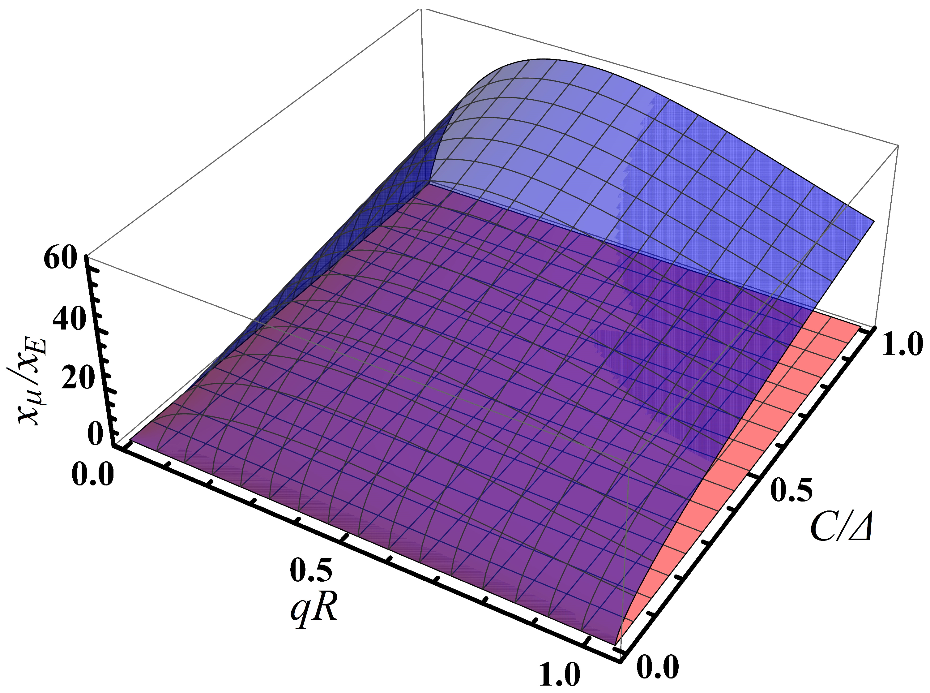
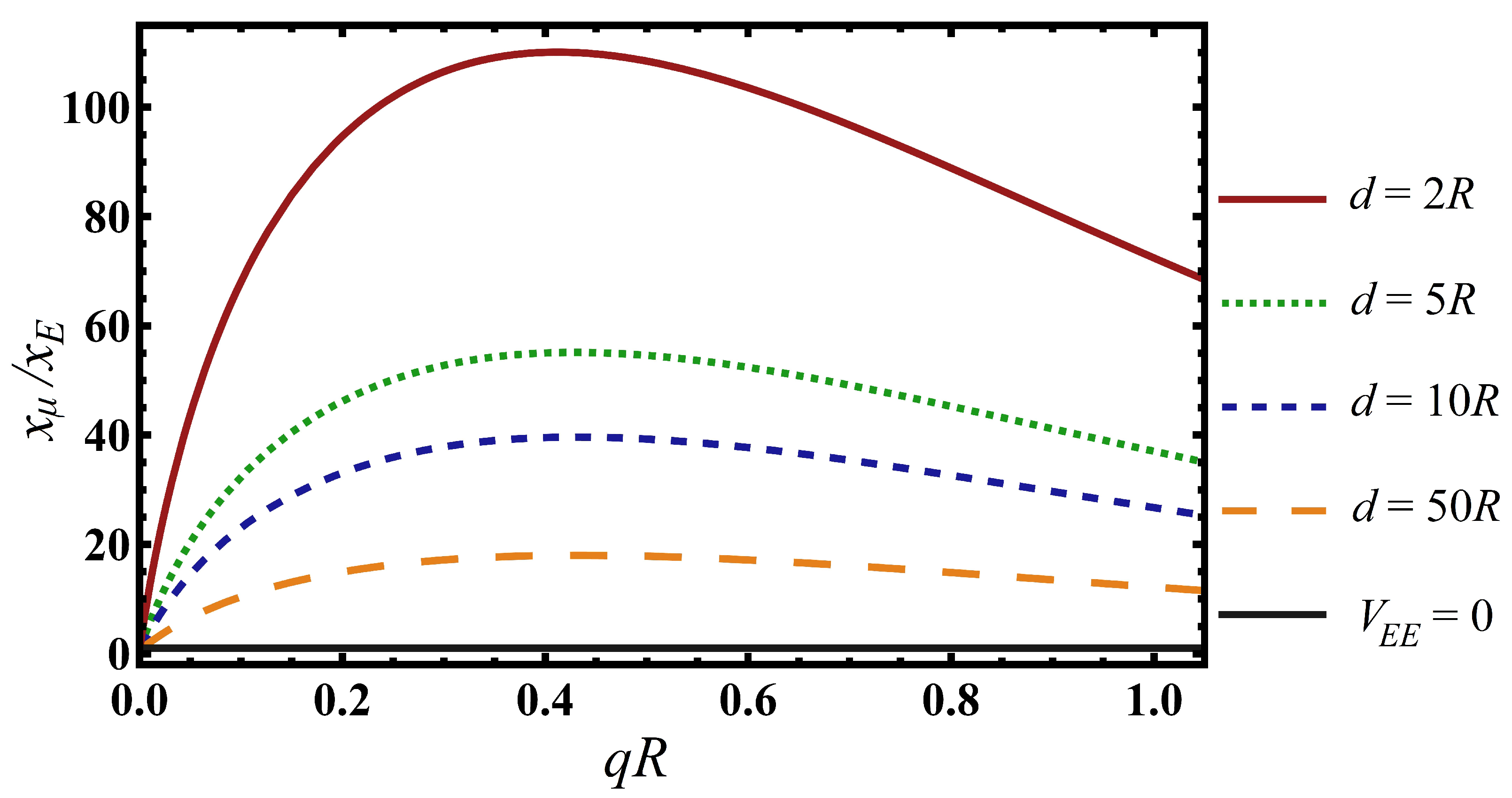
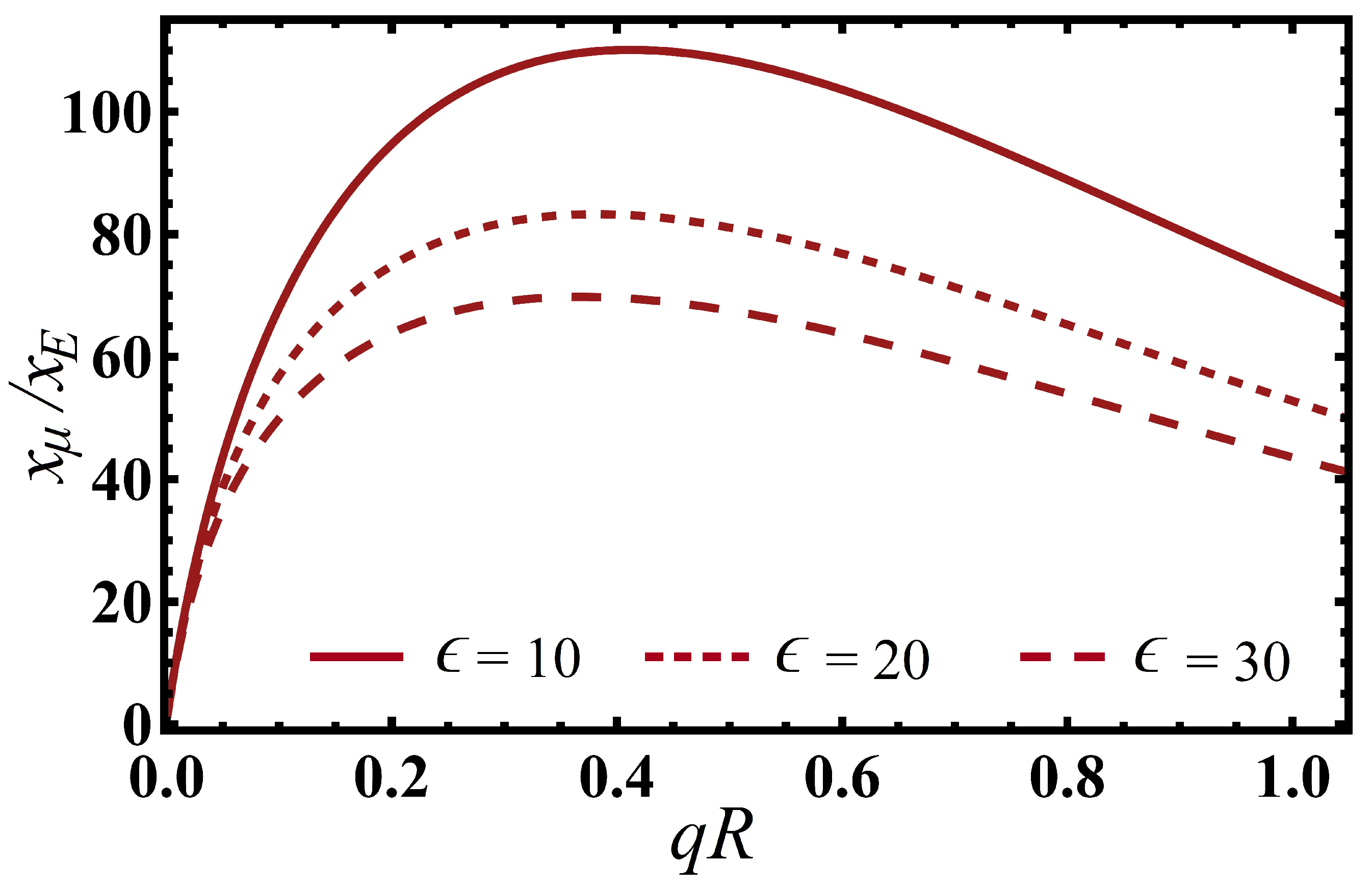
4. Numerical Example: Energy Dispersion of (11,0) SWCNT Film

Qualitative analysis can be helpful for a better understanding of the analytical expressions of dispersion energy, which we have derived in the previous sections. The dispersion relation presented in Section 3 holds for any non-chiral SWCNTs, i.e., both zigzag ( n , 0 ) and armchair ( n , n ) SWCNTs. One can see from Equations (4) and (5) that, if q = 0 , both the SWCNT-plasmon frequency ω p ( 0 , q ) and the interaction potential V E E ( q ) vanish. The intertube center-to-center distance Δ and the thickness of the film d play crucial roles in the energy dispersion of the SWCNT film. Interestingly, the background screening effect does not vanish, even at the minimum value of d and Δ , i.e., d min = 2 R = Δ min . The background screening effect increases if the thickness of the film or the intertube distance increases or if both of them increase.
For illustrative purposes, we considered a periodic homogeneous array of (11,0) zigzag SWCNTs embedded in a dielectric medium of a nominal permittivity value of ϵ = 10 standing in the air ( ϵ 1 = 1 = ϵ 2 ). Our model considers the dielectric medium embedding SWCNTs with a comparatively higher permittivity than substrate and superstrate. One can take a dielectric medium with a permittivity that is an order of magnitude larger than the substrate and superstrate without violating the conditions needed for KR-potential in a transdimensional regime. Silicon ( ϵ = 11.6 ) [36], GaAs ( ϵ = 12.8 ) [36], and SiC ( ϵ = 9.7 ) [37] are some good examples of the dielectric medium in which SWCNTs can be embedded. The radius of an (11,0) SWCNT is R = 11 b / π , in which b = 0.1421 nm is the carbon-carbon nearest neighbor distance, to give the minimum thickness d min 1 nm (=2R) for the (11,0) SWCNT. The zigzag SWCNT’s translational period is a = 3 b / 2 , so that a / R = 3 π / 22 . The quantity γ 0 / e 2 = γ 0 / ( α c ) = 1.874 / nm is a constant, where α , , and c are the fine-structure constant, the reduced Planck constant, and the speed of light in a vacuum, respectively. The dimensionless parameter γ 0 R / e 2 is also of the order of unity for the (11,0)SWCNT.
We considered a homogeneous array of identical (11,0) SWCNTs to exclude possible exciton-plasmon coupling due to other SWCNTs of nearly the same diameter [38]. The discussion presented in Ref. [39] can be implemented to evaluate the quantity E ( e X ( E ) ) 2 for our system as
E ( e X ( E ) ) 2 = 6 π 3 c 3 4 E tot 3 ( q ) τ tot rad ,
where τ ex rad is the exciton-intrinsic radiative lifetime and E tot is the exciton total energy. Thus, the quantity A ( d , Δ , X ( E ) ) becomes
A ( d , Δ , X ( E ) ) A ( d , Δ , q ) = 4 π a d Δ γ 0 E ( e X ( E ) ) 2 = 4 π a d Δ γ 0 6 π 3 c 3 4 E tot 3 ( q ) τ tot rad .
For (11,0) SWCNT, the first Brillouin zone of the longitudinal quasimomentum is given by 2 π / ( 3 b ) q 2 π / ( 3 b ) . The total energy of the ground-internal-state exciton can then be written as presented in Ref. [39], which reads E tot = E exc + 2 π / ( 3 b ) 2 t 2 / ( 2 M ex ) , where the parameter t = 3 q b / ( 2 π ) with 1 t 1 is the dimensionless longitudinal quasimomentum. For (11,0) SWCNT, M ex = 0.44 m 0 , with m 0 being the free-electron mass [40] and t = 1.574 q R . For an (11,0) SWCNT, the quantity 2 π / ( 3 b ) 2 / ( 2 M ex ) evaluates to 0.19 eV , which is about an order of magnitude smaller than the lowest bright exciton energy E exc . For an isolated (11,0) SWCNT, we take τ tot rad = 14.3 ps as presented in Refs. [38,39].
Notice that the solution to the dispersion relation for a system with the chosen homogeneous SWCNTs array, substrate, superstrate, and the dielectric medium is a function of longitudinal quasimomentum. Figure 2 shows the energy eigenvalues in the units of 2 γ 0 as a function of dimensionless momentum and the dimensionless sparseness parameter C / Δ , where C = 2 π R is the circumference of the circular cross-section of the (11,0) SWCNT. The energy value is larger for a closely-packed SWCNT array when the momentum value is larger. As one expects, the energy value ratio x μ / x E tends to unity as Δ and/or q 0 . The energy eigenvalue varies strongly with momentum for thinner SWCNT film, while the energy value varies slowly in comparatively thicker SWCNT film, provided the film is within the TD regime, indicating that the SWCNT energy dispersion is thickness-dependent (See Figure 3). Thickness can be used as a tool in opto-plasmonic device applications, tuning the excitonic energy gap in SWCNT films such that the transdimensional materials are fully compatible with on-chip nanophotonic devices [41]. The thickness dependency of the energy dispersion is lost as the thickness is increased to a 3 D -bulk value. Moreover, the energy dispersion also depends on the dielectric medium in which the CNTs are immersed, as the screening effect increases as the ϵ value of the dielectric increases (see Figure 4).
Of particular interest, the excitonic energy gap at q = 0 is in order. With the aid of Equation (40), one finds from Equation (36) that x μ ± ± x E / 2 as q approaches zero. Similarly, from Equation (2), for q = 0 , one gets x E = E exc / ( 2 γ 0 ) . Using the k · p method of carbon nanotube band theory [35,42], we obtained the first exciton resonance (the lowest energy resonance), E exc at 1.116 eV for an isolated (11,0) SWCNT, which is in good agreement with the experimental value reported in [30]. Thus, for q = 0 , the Δ x μ = E exc / ( 2 γ 0 ) , which for (11,0) SWCNT thin film is 0.207 in the units of 2 γ 0 or 1.116 in electron volts. The calculations were performed at room temperature ( 300 K ).

5. Conclusions

We used the many-particle Green’s function technique and the Matsubara frequency technique to derive an analytical expression for the Hamiltonian of a finite-thickness periodically-aligned SWCNTs array embedded in a dielectric layer with comparatively high permittivity, sandwiched between a substrate and a superstrate of low permittivities. The interaction among the unit cells of different SWCNTs, in addition to the interaction between the unit cells within an SWCNT, makes the problem interesting and challenging. In this paper, we have assumed that the SWCNTs talk with each other through the dipole–dipole interaction. The effective interaction in the SWCNT film is a function of the incident photon’s momentum and the thickness of the film. The effective collective polarization of the film is anisotropic in nature, having predominately larger polarization along the axis of SWCNT alignment and negligible value along the axis perpendicular to SWCNT alignment.
Not all real square matrices have eigenvalues; however, if they have eigenvalues, they can be diagonalized [43]. Some simple approaches, such as (i) solving the characteristic equation of a square matrix and setting the roots as diagonal entries of the matrix or (ii) performing a similarity transformation with the help of an invertible matrix of the same order, may not always be possible. Consequently, one needs a mathematically sophisticated method to diagonalize a mathematically complicated matrix. Using the second quantization method, the Hamiltonian of the film composed of identical periodically-aligned SWCNTs can be expressed in a quadratic form of Bose operators as given in Equation (1), which can be diagonalized by applying the Bogoliubov–Valatin canonical transformation as discussed in Section 4. The energy dispersion in SWCNT film depends on longitudinal quasi-momentum (q), the sparseness of SWCNTs, and the thickness of the film. The exciton energy in the SWCNT film can be controlled and tuned by varying the thickness of the film. The exciton transition band gap also depends on the incident photon’s momentum, permittivities of the dielectric medium, substrate, and superstrate, and the thickness of the film. For a thin film of periodically-aligned (11,0) SWCNTs, the excitonic energy gap for q = 0 is about 1.116 eV.

Author Contributions

Conceptualization, C.M.A.; formal analysis, C.M.A., D.M.M. and T.W.N.; investigation, T.N., B.R.L., and B.R.G.; writing—original draft preparation, C.M.A.; writing—review and editing, All authors; visualization, C.M.A. and T.W.N.; supervision, B.R.G. and C.M.A.; funding acquisition, B.R.G. All authors have read and agreed to the published version of the manuscript.

Funding

This research was funded by NSF RIA program EES 1900998.

Data Availability Statement

Not applicable.

Acknowledgments

This work was supported by NSF RIA program EES 1900998. The authors acknowledge insightful communications with Parameshwari Kattel.

Conflicts of Interest

The authors declare no conflict of interest.

References

  1. Collins, P.G.; Avouris, P. Nanotubes for electronics. Sci. Am. 2000, 62, 283. [Google Scholar] [CrossRef]
  2. Zhang, A.Y. Research on the Properties and Defects of Carbon Nanotubes. In Advanced Materials Research; Trans Tech Publications Ltd.: Wollerau, Switzerland, 2014; Volume 157, p. 971. [Google Scholar]
  3. Hong, S.; Myung, S. Nanotube electronics: A flexible approach to mobility. Nat. Nanotechnol. 2007, 2, 207. [Google Scholar] [CrossRef]
  4. Mintmire, J.W.; Dunlap, B.I.; White, C.T. Are fullerene tubules metallic? Phys. Rev. Lett. 1992, 68, 631. [Google Scholar] [CrossRef] [PubMed]
  5. Lu, X.; Chen, Z. Curved pi-conjugation, aromaticity, and the related chemistry of small fullerenes (<C60) and single-walled carbon nanotubes. Chem. Rev. 2005, 105, 3643. [Google Scholar]
  6. Pop, E.; Mann, D.; Wang, Q.; Goodson, K.; Dai, H. Thermal conductance of an individual single-wall carbon nanotube above room temperature. Nano Lett. 2006, 6, 96. [Google Scholar] [CrossRef] [Green Version]
  7. Ashiba, H.; Iizumi, Y.; Okazaki, T.; Wang, X.; Fujimaki, M. Carbon Nanotubes as Fluorescent Labels for Surface Plasmon Resonance-Assisted Fluoroimmunoassay. Sensors 2017, 17, 2569. [Google Scholar] [CrossRef] [Green Version]
  8. Roberts, J.A.; Yu, S.J.; Ho, P.H.; Schoeche, S.; Falk, A.L.; Fan, J.A. Tunable hyperbolic metamaterials based on self-assembled carbon nanotubes. Nano Lett. 2019, 19, 3131. [Google Scholar] [CrossRef] [PubMed] [Green Version]
  9. Bati, A.S.R.; Yu, L.P.; Tawfik, S.A.; Spencer, M.J.S.; Shaw, P.E.; Batmunkh, M.; Shapter, J.G. Electrically Sorted Single-Walled Carbon Nanotubes-Based Electron Transporting Layers for Perovskite Solar Cells. iScience 2019, 14, 100. [Google Scholar] [CrossRef] [Green Version]
  10. Bondarev, I.V.; Adhikari, C.M. Collective Excitations and Optical Response of Ultrathin Carbon-Nanotube Films. Phys. Rev. Appl. 2021, 15, 034001. [Google Scholar] [CrossRef]
  11. Adhikari, C.M.; Bondarev, I.V. Optical response of ultrathin periodically aligned single-wall carbon nanotube films. Mrs Adv. 2020, 5, 2685. [Google Scholar] [CrossRef]
  12. Keldysh, L.V. Coulomb interaction in thin semiconductor and semimetal films. Engl. Transl. JETP Lett. 1980, 29, 658. [Google Scholar]
  13. Shah, D.; Kudyshev, Z.A.; Saha, S.; Shalaev, V.M.; Boltasseva, A. Transdimensional material platforms for tunable metasurface design. MRS Bull. 2020, 45, 188. [Google Scholar] [CrossRef]
  14. Boltasseva, A.; Shalaev, V.M. Transdimensional Photonics. ACS Photonics 2019, 6, 1. [Google Scholar] [CrossRef] [Green Version]
  15. Mahan, G.D. Many-Particle Physics, 3rd ed.; Kluwer Academic: New York, NY, USA, 2000. [Google Scholar]
  16. Tyablikov, S.V. Method in Quantum Theory of Magnetism; Springer: New York, NY, USA, 1967. [Google Scholar]
  17. Agranivich, V.M. Dispersion of electromagnetic waves in crys tals. J. Exptl. Theoret. Phys. 1959, 37, 430. [Google Scholar]
  18. Philpott, M.R. Diagonalization of a Molecular-Exciton Hamiltonian for an Impure Crystal, Absorption Spectroscopy of Individual Single-Walled Carbon Nanotubes. J. Chem. Phys. 1968, 49, 4537. [Google Scholar] [CrossRef]
  19. Kittel, C. Introduction to Solid State Physics; Wiley: Hoboken, NJ, USA, 2004. [Google Scholar]
  20. Oswald, W.; Wu, Z. Energy gaps in graphene nanomeshes. Phys. Rev. B 2012, 85, 115431. [Google Scholar] [CrossRef] [Green Version]
  21. Goodaire, E.G. Linear Algebra: Pure & Applied; World Scientific Publishing Company: Singapore, 2013. [Google Scholar]
  22. Jentschura, U.D.; Debierre, V.; Adhikari, C.M.; Matveev, A.; Kolachevsky, N. Long-range interactions of hydrogen atoms in excited states. II. Hyperfine-resolved 2S-2S systems. Phys. Rev. A 2017, 95, 022704. [Google Scholar] [CrossRef] [Green Version]
  23. Adhikari, C.M.; Debierre, V.; Jentschura, U.D. Adjacency graphs and long-range interactions of atoms in quasi-degenerate states: Applied graph theory. Appl. Phys. B 2017, 123, 13. [Google Scholar] [CrossRef] [Green Version]
  24. Jentschura, U.D.; Adhikari, C.M. Long-Range Interactions for Hydrogen: 6P-1S and 6P-2S Systems. Atoms 2017, 5, 48. [Google Scholar] [CrossRef] [Green Version]
  25. Jentschura, U.D.; Adhikari, C.M.; Dawes, C.M.; Matveev, A.; Kolachevsky, N. Pressure shifts in high-precision hydrogen spectroscopy. I. Long-range atom-atom and atom-molecule interactions. J. Phys. B At. Mol. Opt. Phys. 2019, 52, 075005. [Google Scholar] [CrossRef]
  26. Adhikari, C.M.; Jentschura, U.D. Long-Range Interactions for Hydrogen Atoms in Excited D States. Atoms 2022, 10, 6. [Google Scholar] [CrossRef]
  27. Amori, A.R.; Hou, Z.; Krauss, T.D. Excitons in Single-Walled Carbon Nanotubes and Their Dynamics. Annu. Rev. Phys. Chem. 2018, 69, 81. [Google Scholar] [CrossRef]
  28. Umari, P.; Petrenko, O.; Taioli, S.; De Souza, M.M. Communication: Electronic band gaps of semiconducting zig-zag carbon nanotubes from many-body perturbation theory calculations. J. Chem. Phys. 2012, 136, 181101. [Google Scholar] [CrossRef] [Green Version]
  29. Kilina, S.; Badaeva, E.; Piryatinski, A.; Tretiak, S.; Saxena, A.; Bishop, A.R. Bright and dark excitons in semiconductor carbon nanotubes: Insights from electronic structure calculations. Phys. Chem. Chem. Phys. 2009, 11, 4113. [Google Scholar] [CrossRef]
  30. Weisman, R.B.; Bachilo, S.M. Dependence of Optical Transition Energies on Structure for Single-Walled Carbon Nanotubes in Aqueous Suspension: An Empirical Kataura Plot. Nano Lett. 2003, 3, 1235. [Google Scholar] [CrossRef]
  31. Cubukcua, E.; Degirmencia, F.; Kocabasb, C.; Zimmlera, M.A.; Rogersc, J.A.; Capasso, F. Aligned carbon nanotubes as polarization-sensitive, molecular near-field detectors. Proc. Natl. Acad. Sci. USA 2009, 106, 2495. [Google Scholar] [CrossRef] [Green Version]
  32. Benedict, L.X.; Louie, S.G.; Cohen, M.L. Static polarizabilities of single-wall carbon nanotubes. Phys. Rev. B 1995, 52, 8541. [Google Scholar] [CrossRef]
  33. Kozinsky, B.; Marzari, N. Static dielectric properties of carbon nanotubes from first principles. Phys. Rev. Lett. 2006, 96, 166801. [Google Scholar] [CrossRef] [Green Version]
  34. Sasaki, K.-I.; Riichiro Saito, R. Pseudospin and Deformation-Induced Gauge Field in Graphene. Prog. Theor. Phys. Suppl. 2008, 176, 253. [Google Scholar] [CrossRef]
  35. Marconcini, P.; Macucci, M. The k · p method and its application to graphene, carbon nanotubes andgraphene nanoribbons: The Dirac equation. Riv. Nuovo Cim. 2011, 34, 489. [Google Scholar]
  36. Karlheinz, S. Microwave dielectric constants of silicon, gallium arsenide, and quartz. J. Appl. Phys. 1988, 63, 5439. [Google Scholar]
  37. Kazimierczuk, M.K. Pulse-Width Modulated DC-DC Power Converters; Wiley: Weinheim, Germany, 2015. [Google Scholar]
  38. Adhikari, C.M.; Bondarev, I.V. Controlled exciton–plasmon coupling in a mixture of ultrathin periodically aligned single-wall carbon nanotube arrays. J. Appl. Phys. 2021, 129, 015301. [Google Scholar] [CrossRef]
  39. Bondarev, I.V.; Woods, L.M.; Tatur, K. Strong exciton-plasmon coupling in semiconducting carbon nanotubes. Phys. Rev. B 2009, 80, 085407. [Google Scholar] [CrossRef] [Green Version]
  40. Spataru, C.D.; Ismail-Beigi, S.; Capaz, R.B.; Louie, S.G. Theory and Ab Initio Calculation of Radiative Lifetime of Excitons in Semiconducting Carbon Nanotubes. Phys. Rev. Lett. 2005, 95, 247402. [Google Scholar] [CrossRef] [Green Version]
  41. Dong, S.; Zhang, Q.; Cao, G.; Ni, J.; Shi, T.; Li, S.; Duan, J.; Wang, J.; Li, Y.; Sun, S.; et al. On-chip trans-dimensional plasmonic router. Nanophotonics 2020, 9, 3357. [Google Scholar] [CrossRef]
  42. Ando, T. Theory of Electronic States and Transport in Carbon Nanotubes. J. Phys. Soc. Jpn. 2005, 74, 777. [Google Scholar] [CrossRef] [Green Version]
  43. Saad, Y. Numerical Methods for Large Eigenvalues Problems; Society for Industrial and Applied Mathematics: Philadelphia, PA, USA, 2011. [Google Scholar]
Figure 1. Schematic diagram showing our model system, which consists of a periodic array of identical SWCNTs of radius R and length L. L and d are the width of the film and its thickness. ϵ 1 , ϵ 2 , and ϵ are permittivities of the substrate, superstrate, and the dielectric medium in which SWCNT film is embedded. Δ is the center-to-center distance between two adjacent carbon nanotubes.
Condensedmatter 08 00053 g001
Figure 2. Figure shows solutions to the energy dispersion relation in terms of dimensionless energy ratio x μ / x E , as a function of the dimensionless momentum q R and carbon nanotubes sparseness in terms of circumference C to the center-to-center SWCNT distance Δ ratio for a homogeneous periodic array of (11,0) SWCNTs.
Condensedmatter 08 00053 g002
Figure 3. Figure shows solutions to the energy dispersion relation in terms of dimensionless energy ratio x μ / x E , as a function of the dimensionless momentum q R for a closely-packed homogeneous periodic array of (11,0) SWCNTs for different thicknesses of the film. V E E = 0 represents the case in which the interaction among SWCNTs is switched off.
Condensedmatter 08 00053 g003
Figure 4. Figure shows solutions to the energy dispersion relation in terms of dimensionless energy ratio x μ / x E , as a function of the dimensionless momentum q R for a closely packed homogeneous periodic array of (11,0) SWCNTs for an ultrathin film of thickness d = 2 R with interlude center-to-center distance Δ = 2 R for three different dielectric mediums with ϵ = 10, 20, and 30.
Condensedmatter 08 00053 g004
Disclaimer/Publisher’s Note: The statements, opinions and data contained in all publications are solely those of the individual author(s) and contributor(s) and not of MDPI and/or the editor(s). MDPI and/or the editor(s) disclaim responsibility for any injury to people or property resulting from any ideas, methods, instructions or products referred to in the content.

