Article

Rabi Coupled Fermions in the BCS–BEC Crossover

by
Luca Dell’Anna
1,2,*,
Federico De Bettin
1 and
Luca Salasnich
1,2,3
1
Dipartimento di Fisica e Astronomia “G. Galilei” and QTech Center, Università di Padova, Via Marzolo 8, 35131 Padova, Italy
2
Istituto Nazionale di Fisica Nucleare, Sezione di Padova, Via Marzolo 8, 35131 Padova, Italy
3
Istituto Nazionale di Ottica del Consiglio Nazionale delle Ricerche, Via Nello Carrara 2, 50019 Sesto Fiorentino, Italy
*
Author to whom correspondence should be addressed.
Condens. Matter 2022, 7(4), 59; https://doi.org/10.3390/condmat7040059
Submission received: 14 September 2022 / Revised: 16 October 2022 / Accepted: 18 October 2022 / Published: 22 October 2022

Abstract

:
We investigate the three-dimensional BCS–BEC crossover in the presence of a Rabi coupling, which strongly affects several properties of the system, such as the chemical potential, the pairing gap and the superfluid density. We determine the critical interaction strength, below which the system is normal also at zero temperature. Finally, we calculate the effect of the Rabi coupling on the critical temperature of the superfluid-to-normal phase transition by using different theoretical schemes.

1. Introduction

An extremely important achievement in the field of ultracold atoms has been the realization of the crossover from the Bardeen–Cooper–Schrieffer (BCS) superfluid phase of loosely bound pairs of fermions to the Bose–Einstein condensate (BEC) of tightly bound composite bosons [1]. Recently a renewed interest in this field has been triggered by a breakthrough experiment [2] showing that the spin of an atom could be coupled to its center-of-mass motion by dressing two atomic spin states with a pair of laser beams. This technique has been then adopted in other experimental investigations of bosonic [3] and fermionic [4] atomic gases with artificial spin-orbit and Rabi coupling. Triggered by this pioneering remarkable experiment in the last few years, a large number of theoretical papers have analyzed, within a mean field approach, the effect of spin-orbit couplings of Rashba [5] and Dresselhaus [6] type, often with the inclusion of a Rabi term, in the condensates [7,8,9,10,11,12] and in the BCS–BEC crossover of superfluid fermions [4,13,14,15,16,17,18,19,20,21,22,23,24,25,26,27,28,29]. In particular, a spin-orbit coupling can turn a first-order phase transition driven by a Rabi coupling into a second-order one.
The aim of this paper is, instead, the study of an ultracold gas of purely Rabi coupled fermionic atoms interacting via a two body contact potential. We consider a gas of identical atoms characterized by two hyperfine states. The entire atomic sample is continuously irradiated by a wide laser beam. The laser frequency is in near resonance with the Bohr frequency of the two hyperfine states of each atom. In this way, there is persistent periodic transition between the two atomic quantum states with frequency ω R , that is, the Rabi frequency which is proportional to the atomic dipole moment of the transition and to the amplitude of the laser electric field. The itinerant ferromagnetism of repulsive fermions with Rabi coupling was studied in both two [30] and three [31] spatial dimensions. Here, instead, we want to investigate the interplay of Rabi coupling and attractive interaction for fermions in the three-dimensional BCS–BEC crossover. It is important to stress that if one considers a new spin basis of symmetric and anti-symmetric superpositions of the bare spin states, then the Rabi term behaves as an effective Zeeman field that breaks the balance of the two new spin components (see, for instance, Ref. [32]). This spin-imbalanced attractive fermionic system has been previously investigated [33,34]. The current work adds new insights into the problem, not only because the physical setup is different, but also because we analyze in detail, as a function of the Rabi coupling, the critical interaction strength below which the system is in the normal phase also at zero temperature, the equation of state, the superfluid fraction, and two alternative ways to determine the beyond-mean-field critical temperature. In Section 2 we introduce Rabi coupling in the model of attractive fermions. In Section 3 we investigate the problem at the mean field level, also considering an improved determination [35] of the critical temperature of the superfluid-to-normal phase transition. In Section 4 we consider beyond-mean-field corrections and use them to calculate the critical temperature with the inclusion of Gaussian fluctuations [28,36].

2. The Model

Our ultracold Fermi gas model is enriched with the addition of Rabi coupling, which enables the spin of the particles involved to flip. The Euclidean action, omitting the explicit dependence of the fermionic fields ψ σ ( r , τ ) ( σ = , ) on space r and imaginary time τ , then, reads:
S [ ψ ¯ , ψ ] = 0 β d τ V d 3 r ψ ¯ σ τ 2 2 m μ ψ σ g ψ ¯ ψ ¯ ψ ψ + ω R ( ψ ¯ ψ + ψ ¯ ψ ) ,
where β = 1 / ( k B T ) with T the temperature and k B the Boltzmann constant, μ is the chemical potential and V is the volume. Notice that in this paper we set = 1 . Within the path integral formalism, the partition function of the system is given by:
Z = D [ ψ ¯ , ψ ] e S [ ψ ¯ , ψ ] ,
and from the partition function Z all the thermodynamical quantities can be derived.
We perform a Hubbard–Stratonovich transformation, so that the model can be rewritten in terms of a new action depending also on a new spinless complex field Δ ( r , τ ) :
S [ Δ ¯ , Δ , ψ ¯ , ψ ] = 0 β d τ V d 3 r | Δ ( r , τ ) | 2 g 1 2 Ψ ¯ ( r , τ ) G 1 Ψ ( r , τ ) + β p ξ p ,
where ξ p = p 2 / ( 2 m ) μ is the shifted single-particle energy and the Nambu spinors take the form:
Ψ ( r , τ ) = ψ ( r , τ ) ψ ¯ ( r , τ ) ψ ( r , τ ) ψ ¯ ( r , τ ) ,
while the inverse fermionic propagator is:
G 1 = τ + 2 2 m + μ Δ ( r , τ ) ω R 0 Δ ¯ ( r , τ ) τ 2 2 m μ 0 ω R ω R 0 τ + 2 2 m + μ Δ ( r , τ ) 0 ω R Δ ¯ ( r , τ ) τ 2 2 m μ .
The action is now Gaussian in the fermionic degrees of freedom; therefore, we can integrate over them obtaining an effective theory for the complex field Δ , whose action reads:
S eff [ Δ ¯ , Δ ] = 0 β d τ V d 3 r | Δ ( r , τ ) | 2 g 1 2 Tr ln ( G 1 ) + β p ξ p .
It is also convenient and useful for what follows to write G 1 in Fourier space, after denoting the four momenta by capital letters, such as P = ( i ν n , p ) , introducing the fermionic Matsubara frequencies, ν n = ( 2 n + 1 ) π β , with n Z . From Equation (5), we find that the Fourier components of the inverse fermionic propagator G K P 1 reads, therefore:
( i ν n ξ p ) δ K , P Δ K + P ω R δ K , P 0 Δ ¯ K + P ( i ν n + ξ p ) δ K , P 0 ω R δ K , P ω R δ ( K , P ) 0 ( i ν n ξ p ) δ K , P Δ K + P 0 ω R δ K , P Δ ¯ K + P ( i ν n + ξ p ) δ K , P .

3. Mean Field Approach

We can now perform, from Equation (6), the saddle point approximation, choosing Δ = Δ 0 , namely homogeneous in space and time and, without lack of generality, fixing it real. The mean field action, then, reads:
S mf = β V Δ 0 2 g 1 2 Tr ln ( G 1 ) + β p ξ p ,
where G 0 1 is equal to G 1 where we take Δ = Δ 0 . It is convenient working in Matsubara representation so that:
det ( G 0 1 ) = ν n 2 + ( ω p ) 2 ν n 2 + ( ω p ) 2 ,
with
ω p + = ξ p 2 + Δ 0 2 + ω R ,
ω p = ξ p 2 + Δ 0 2 ω R .
These two energies correspond to the poles of the fermionic propagator after a Wick rotation, meaning that they are the single particle excitation energies of the theory, and they differ from the case without Rabi coupling only by a constant shift ω R . The presence of Rabi coupling splits the excitation energies into two different energy levels separated by a shift 2 ω R . It is immediately clear that ω p may take negative values, which is somewhat unexpected. This may happen for Δ 0 < ω R , a regime which is unphysical, as we will see, unless Δ 0 = 0 .
The mean-field grand potential is given by:
Ω mf = k B T S mf .
Explicitly, we have:
Ω mf = V Δ 0 2 g 1 2 ν n , p ln ν n 2 + ( ω p + ) 2 + ln ν n 2 + ( ω p ) 2 ,
where we used Tr ln ( G 0 1 ) = ln det ( G 0 1 ) and Equation (9). After summing over the Matsubara frequencies, we get:
Ω mf V = Δ 0 2 g k B T 2 V p ln 2 1 + cosh ( β ω p + ) + ln 2 1 + cosh ( β ω p ) .

3.1. Gap and Number Equations

Minimizing the mean-field grand potential Ω mf with respect to Δ 0 , we obtain the so-called gap equation:
1 g = 1 4 V p tanh β 2 ω p + ξ p 2 + Δ 0 2 + tanh β 2 ω p ξ p 2 + Δ 0 2 .
This equation is divergent in the ultraviolet and requires a regularization of the interaction strength g, namely:
1 g = m 4 π a F + 1 V p m p 2 ,
with a F being the physical s-wave scattering length.
The total number density n is instead obtained by:
n = 1 V Ω mf μ ,
which is the so-called number equation. The sum over Matsubara frequencies has the same form as the one of the gap equation. After some manipulations, the renormalized gap equation and the number equation reads:
m V 4 π a F = p tanh β 2 ω p + + tanh β 2 ω p 4 ξ p 2 + Δ 0 2 m p 2
n V = p 1 ξ p 2 tanh β 2 ω p + + tanh β 2 ω p ξ p 2 + Δ 0 2 .
The difference with respect to the case without Rabi coupling is a shift of ± ω R in the arguments of the hyperbolic tangents, which makes the derivation of analytic results more demanding.

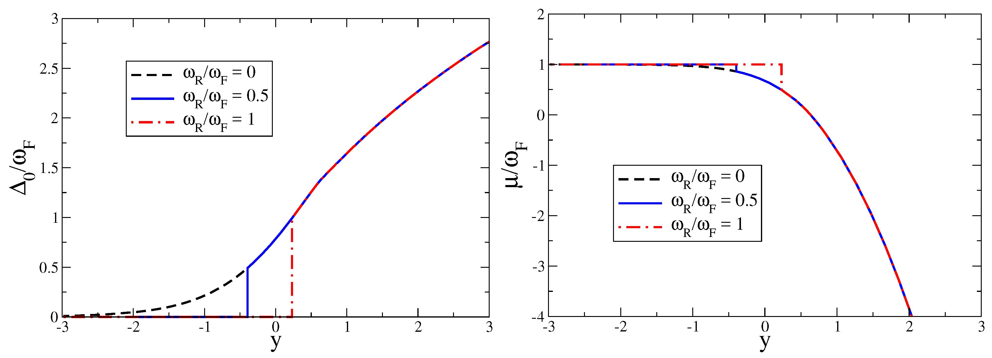
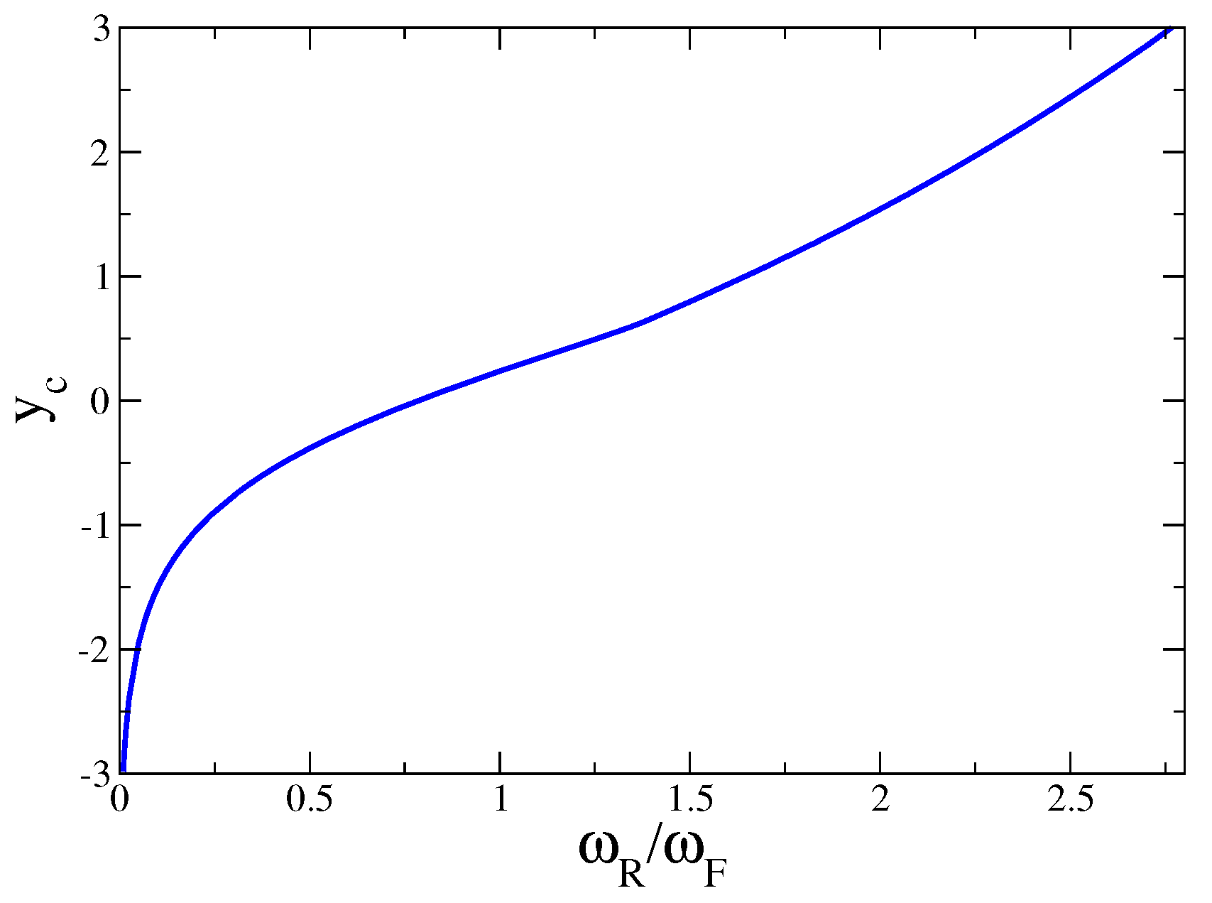
3.2. Zero Temperature

At zero temperature, Equations (18) and (19) simplify because the hyperbolic tangent goes to one for T 0 + . However, careful attention should be paid to studying the sign of ω p , which affects the form of the equations. In fact, if ω p > 0 for any value of the momentum p , the number and gap equations will take the same form as the ones with no Rabi interaction, while if for some values of p the energy ω p < 0 , the equations will take a different form, as we will show below. The main result of this zero-temperature analysis is the following: (i) if Δ 0 < ω R , the Rabi frequency ω R changes the momenta domain of integration in the equations in such a way that the gap equation has no finite solutions; (ii) if Δ 0 > ω R , instead, the Rabi frequency ω R does not affect the gap and the number equations.
In Figure 1, we report the plots of the energy gap Δ 0 (left panel) and chemical potential μ (right panel) as functions of the s-wave scattering length a F . There results are then analogous to the ones in the case without Rabi coupling for Δ 0 > ω R , but exhibit a different behaviour below such a threshold. In particular, both these quantities, the energy gap Δ 0 and the chemical potential μ , for a small range of 1 / ( k F a F ) , have two branches. However, the stable branch (associated to the minima of the grand potential Ω ) is the upper branch shown in the figures, superimposed on the curves of ω R = 0 . The unstable is not reported.
At zero temperature ( T = 0 ), the main effect of the Rabi coupling ω R is, therefore, to make the system normal, i.e., with Δ 0 = 0 , for 1 / ( k F a F ) y c , where y c = for ω R = 0 . The critical strength y c grows by increasing ω R . Specifically, given Δ 0 ( y ) with 1 / ( k F a F ) for ω R = 0 , y c is obtained from the condition Δ 0 ( y c ) = ω R . This means that inverting the plot of Δ 0 ( y ) (obtained for ω R = 0 ) one gets immediately y c vs. ω R , as shown, for the sake of completeness, in Figure 2.

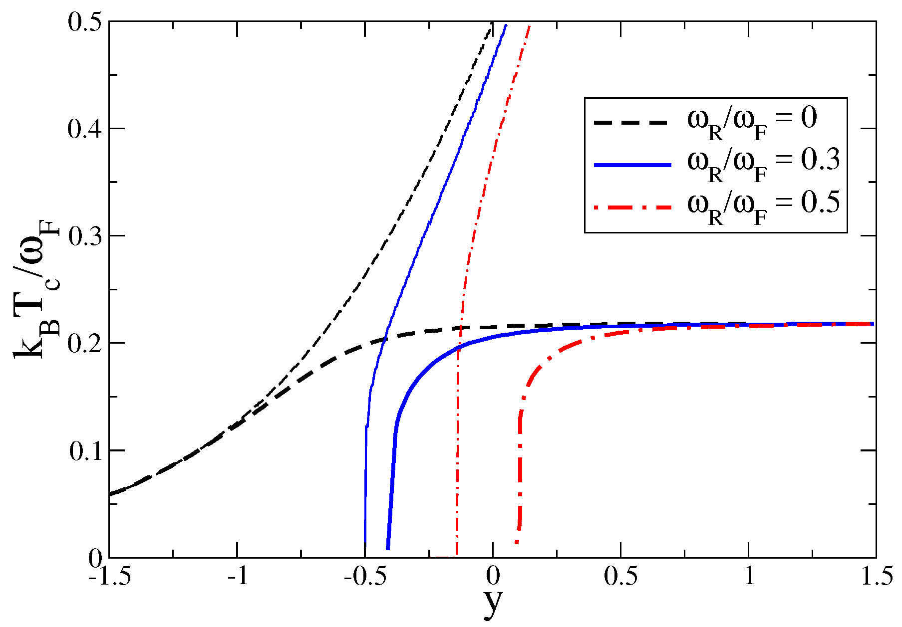
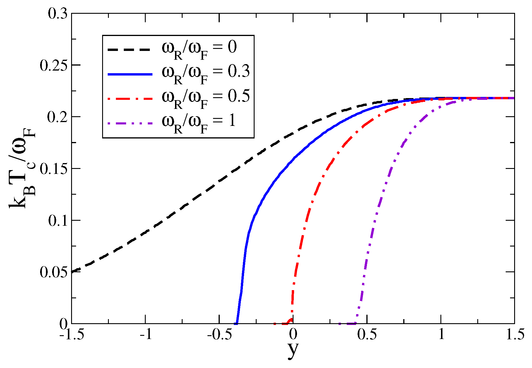
3.3. Critical Temperature

We now investigate the behaviour of the system at the critical temperature T c , at which the energy gap Δ 0 ( T c ) = 0 . Let us define, for simplicity, the following adimensional quantities: μ ˜ = μ / ω F , T ˜ c = k B T c / ω F , ω ˜ R = ω R / ω F and y = 1 / ( k F a F ) . In this case the gap and the number equations can be written as follows:
y = 2 T ˜ c 2 π J 3 μ ˜ , T ˜ c , ω ˜ R ,
T ˜ c = 4 J 4 μ ˜ , T ˜ c , ω ˜ R 2 / 3 ,
where
J 3 = 0 + d x x 2 tanh 1 2 ( x 2 μ ˜ T ˜ c + ω ˜ R T ˜ c ) 2 ( x 2 μ ˜ T ˜ c ) + tanh 1 2 ( x 2 μ ˜ T ˜ c ω ˜ R T ˜ c ) 2 ( x 2 μ ˜ T ˜ c ) 1 x 2
and
J 4 = 0 + d x x 4 1 cosh 2 1 2 ( x 2 μ ˜ T ˜ c + ω ˜ R T ˜ c ) + 1 cosh 2 1 2 ( x 2 μ ˜ T ˜ c ω ˜ R T ˜ c ) .
Solving the coupled Equations (20) and (21), we obtain the critical temperature T c as a function of the inverse scattering length 1 / a F for different values of the Rabi coupling ω R . The results are shown as thin curves in Figure 3.
As expected, the Rabi coupling inhibits the formation of Cooper pairs: the stronger the Rabi coupling, the higher is the threshold of the scattering rate above which superfluidity can occur at the mean field level. In the strong coupling limit, instead, even in the absence of Rabi coupling, the mean field approach is expected to fail since it cannot describe the emergence of bosonic molecules which undergo condensation below a finite critical temperature. We have, therefore, to go beyond the mean field approximation.

4. Beyond Mean Field

We now present a couple of techniques which allow us to go beyond the mean field analysis. The first approach is a method based on the determination of the superfluid density, while the second one is based on the inclusion of the Gaussian fluctuations. In the latter case, we will show some explicit results in the so-called bosonic approximation.

4.1. By Superfluid Density

An improved determination of the critical temperature T c can be obtained with the method proposed by Babaev and Kleinert [35], which is the three-dimensional analog of the Nelson–Kosterlitz criterion. In particular,
k B T c = α n s ( T c ) 4 m 2 n 1 / 3 ,
where n s ( T ) is the mean-field superfluid density and n is the total fermionic number density. Actually, J = n s / ( 4 m ) is the stiffness in an effective XY model, H = J 2 d r θ ( r ) , where θ is the local phase of the pairing Δ .
The constant α is fixed to the value α = 2 π / ζ ( 3 / 2 ) 2 / 3 such that T c turns out to be the exact value k B T c = π / m ( n / ( 2 ζ ( 3 / 2 ) ) ) 2 / 3 for n / 2 non-interacting bosons with mass 2 m in the deep BEC regime. The superfluid density n s ( T ) can be calculated, following the Landau’s approach [37], getting:
n s ( T ) = n + 1 6 d 3 p ( 2 π ) 3 p 2 m d f B ( ω p + ) d ω p + + d f B ( ω p ) d ω p
where
f B ( ω ) = 1 e β ω 1
is the Bose–Einstein distribution and n is the total number density. The thick curves of Figure 3 are obtained using Equation (24) with Equation (25), where Δ 0 and μ are numerically determined from Equations (18) and (19).
As done previously, it is convenient to introduce adimensional quantities, μ ˜ = μ / ω F , T ˜ c = k B T c / ω F , ω ˜ R = ω R / ω F and y = 1 / ( k F a F ) together with Δ ˜ 0 = Δ 0 / ω F , where we recall that ω F = k F 2 / ( 2 m ) = ( 3 π 2 n ) 2 / 3 / ( 2 m ) . We can, therefore, rewrite Equation (24) as:
T ˜ c = 2 ( 6 π ζ ( 3 / 2 ) ) 2 / 3 n s ( T ˜ c ) n
which, in the deep BEC where all the fermions contribute to the superfluid density, gives T ˜ c 0.218 , and where
n s ( T ˜ c ) n = 1 1 2 T ˜ c s = ± 1 0 + d x x 4 e 1 T ˜ c ( x 2 μ ˜ ) 2 + Δ ˜ 0 2 + s ω ˜ R e 1 T ˜ c ( x 2 μ ˜ ) 2 + Δ ˜ 0 2 + s ω ˜ R 1 2

4.2. Gaussian Fluctuations

We now introduce Gaussian fluctuations in the partition function of the system adopting the Nozieres–Schmitt–Rink approach [36]. The aim is to derive a more precise form for the number equation in order to understand the role of quantum fluctuations on the relation between the chemical potential μ and the density n of fermions.
In order to introduce fluctuations, we separate the field Δ ( r , τ ) in its homogeneous part Δ 0 , obtained minimizing the grand potential at the mean field level, and its small fluctuations η ( r , τ ) around the saddle point solution,
Δ ( r , τ ) = Δ 0 + η ( r , τ ) .
After some calculations, at the leading order in η , the effective action Equation (6) at the Gaussian level reads:
S eff S mf + 1 2 Q η ¯ Q η Q M Q η Q η ¯ Q ,
with
M Q = 1 g I + χ Q ,
where χ Q is the contribution coming from the expansion of Tr ln ( G 1 ) and I denotes the 2 × 2 identity matrix in Nambu space. The components of χ Q , shown in Appendix A, depend on the the quadrivector Q = ( i υ n , q ) , where υ n are bosonic Matsubara frequencies, υ n = 2 π n β , with n Z .
Our objective is to find an expression for the grand canonical potential from which we can recover a treatable expression for the contribution of the Gaussian fluctuations to the number equation. The effective theory we obtained is Gaussian, meaning that it can be integrated explicitly, getting the following partition function:
Z = e S mf Q det ( M Q ) 1 .
The grand potential, then, reads:
Ω = Ω mf + Ω g ,
where Ω mf is given by Equation (12) and
Ω g = k B T Q ln [ det ( M Q ) ] .
To compute the sum over Matsubara frequencies in (34), one may analytically continue the argument of the sum by setting i υ n ω and transforming the sum into an integral. In this way we eventually find
Ω g = 1 π q + d ω f B ( ω ) δ ˜ ( ω , q )
with f B ( ω ) the Bose–Einstein distribution and
δ ˜ ( ω , q ) = a r c t a n I m [ det [ M ω , q ] R e [ det [ M ω , q ] ,
the phase of the complex metrix element M ω , q derived from (31). Thus, the Gaussian correction to the number density reads:
n g = 1 V Ω g μ = 1 π V q + d ω f B ( ω ) δ ˜ ( ω , q ) μ .
In the strong coupling limit a F 0 + the system becomes a gas of free bosonic dimers, made of two fermions with opposite spin and binding energy E B = 1 / ( m a F 2 ) . These bosons have mass m B = 2 and chemical potential μ B = 2 μ E B . Indeed, as shown in Ref. [28], in this regime μ B 0 and
δ ˜ ( ω , q ) μ π δ ω q 2 2 m B + μ B ,
where δ ( x ) is the Dirac delta function. It follows immediately that, in the strong coupling approximation, also called bosonic approximation [28], the number equation with Gaussian fluctuations becomes:
n V = p 1 ξ p 2 tanh β 2 ω p + + tanh β 2 ω p ξ p 2 + Δ 0 2 + q 1 e β ( q 2 4 m μ B ) 1 .
In Figure 4, we report the critical temperature T c as a function of the inverse scattering length 1 / a F obtained by solving Equations (18) and (39), setting μ B = 0 and Δ 0 = 0 . The full calculation of Equation (37) is more computationally demanding and is expected to deviate from the bosonic approximation only in the intermediate regime near unitarity limit ( y = 0 ) producing a little hump in the T c profile, which is, however, a debated feature within other theoretical schemes [38].

5. Conclusions

The BCS–BEC crossover has been studied in the presence of Rabi coupling by using the finite-temperature path integral formalism. The behavior of many physical quantities has been studied along the whole crossover, including the mean-field chemical potential and energy gap at zero temperature, and the critical temperature at and beyond mean-field level. We have found that only in the deep BEC regime are the physical properties of the system not affected by the Rabi coupling. In general, also at zero temperature, there exists a critical interaction strength, below which the system is normal. We have determined this critical strength as a function of the Rabi coupling. In the last part of the paper we have calculated the critical temperature of the superfluid-to-normal phase transition for different values of the Rabi coupling. The treatment beyond mean-field level has been carried out following two different procedures: the Babaev–Kleinert [35] and the Nozieres–Schmitt–Rink [36] approaches: the first is based on the determination of the mean-field superfluid density as a function of the temperature while the second is more rigorous but computationally demanding. Indeed, the Nozieres–Schmitt–Rink scheme has been used, but adopts the bosonic pair approximation [28], which makes the scheme more feasible numerically.

Author Contributions

Conceptualization, L.S., L.D.; Formal analysis, L.D., F.D.B., L.S.; Investigation L.D., F.D.B., L.S.; Methodology, L.D., F.D.B., L.S.; Writing, L.D., F.D.B., L.S. All authors have read and agreed to the published version of the manuscript.

Funding

This work was supported by the BIRD project “Ultracold atoms in curved geometries” of the University of Padova.

Data Availability Statement

Not applicable.

Acknowledgments

L.S. acknowledges the BIRD project “Ultracold atoms in curved geometries” of the University of Padova for partial support.

Conflicts of Interest

The authors declare no conflict of interest.

Appendix A

Let us write the fermionic propagator, including quantum fluctuations, as follows
G 1 = G 0 1 + η ^ = G 0 1 ( 1 + G 0 η ^ )
where we introduce the matrix
η ^ Q = 0 η Q 0 0 η ¯ Q 0 0 0 0 0 0 η Q 0 0 η ¯ Q 0 .
so that, in the action, the Tr ln ( G 1 ) can be written in the following way
1 2 Tr ln ( G 1 ) = 1 2 Tr ln ( G 0 1 ) + 1 2 Tr ln ( 1 + G 0 η ^ ) .
We can now expand the last term, getting the following leading term
1 2 Tr G 0 η ^ G 0 η ^ = k B T V Q , P tr ( G 0 P η ^ Q G 0 P + Q η ^ Q )
which can be recasted, performing the matrix products, as follows
1 2 Tr G 0 η ^ G 0 η ^ = 1 2 Q η ¯ Q η Q χ Q η Q η ¯ Q
where χ Q is a 2 × 2 matrix, introduced in the main text in Equation (31), which, after performing the inverse of G 0 1 and making the matrix products, can be written explicitly. This matrix is composed by the following diagonal terms (see Ref. [39] for more details)
( χ Q ) 11 = ( χ Q ) 22 = k B T V p , ν n [ ( i ν n ξ p ) ( ( i ν n ) 2 ξ p 2 Δ 0 2 ) ω R 2 ( i ν n + ξ p ) ] ( ν n 2 + ( ω p + ) 2 ) ( ν n 2 + ( ω p ) 2 ) × [ ( i υ m + i ν n + ξ q + p ) ( ( i υ m + i ν n ) 2 ξ q + p 2 Δ 0 2 ) ω R 2 ( i υ m + i ν n ξ q + p ) ] ( ( υ m + ν n ) 2 + ( ω q + p + ) 2 ) ( ( υ m + ν n ) 2 + ( ω q + p ) 2 + ω R 2 k B T V p , ν n [ Δ 0 2 ω R 2 + ( i ν n ξ p ) 2 ] ( ν n 2 + ( ω p + ) 2 ) ( ν n 2 + ( ω p ) 2 ) [ Δ 0 2 ω R 2 + ( i υ m + i ν n + ξ p + q ) 2 ] ( ( υ m + ν n ) 2 + ( ω q + p + ) 2 ) ( ( υ m + ν n ) 2 + ( ω q + p ) 2 )
and off-diagonal terms
( χ Q ) 12 = ( χ Q ) 21 = Δ 0 2 k B T V p , ν n ( ν n 2 + ξ p 2 ) ω R 2 + Δ 0 2 ( ν n 2 + ( ω p + ) 2 ) ( ν n 2 + ( ω p ) 2 ) × ( ( υ m + Ω n F ) 2 + ξ p + q 2 ) ω R 2 + Δ 0 2 ( ( υ m + ν n ) 2 + ( ω q + p + ) 2 ) ( ( υ m + ν n ) 2 + ( ω q + p ) 2 ) 4 ω R 2 Δ 0 2 k B T V p , ν n ν n ( ν n 2 + ( ω p + ) 2 ) ( ν n 2 + ( ω p ) 2 ) × ( υ m + ν n ) ( ( υ m + ν n ) 2 + ( ω q + p + ) 2 ) ( ( υ m + ν n ) 2 + ( ω q + p ) 2 ) .

References

  1. Zwerger, W. The BCS–BEC Crossover and the Unitary Fermi Gas; Springer: Berlin/Heidelberg, Germany, 2012. [Google Scholar]
  2. Lin, Y.J.; Jimenez-Garcia, K.; Spielman, I.B. Spin–orbit-coupled Bose–Einstein Condensates. Nature 2011, 471, 83. [Google Scholar] [CrossRef] [Green Version]
  3. Zhang, J.-Y.; Ji, S.-C.; Chen, Z.; Zhang, L.; Du, Z.-D.; Yan, B.; Pan, G.-S.; Zhao, B.; Deng, Y.-J.; Zhai, H.; et al. Collective Dipole Oscillations of a Spin-Orbit Coupled Bose-Einstein Condensate. Phys. Rev. Lett. 2012, 109, 115301. [Google Scholar] [CrossRef] [PubMed]
  4. Wang, P.; Yu, Z.-Q.; Fu, Z.; Miao, J.; Huang, L.; Ghai, S.; Zhai, H.; Zhang, J. Spin-Orbit Coupled Degenerate Fermi Gases. Phys. Rev. Lett. 2012, 109, 095301. [Google Scholar] [CrossRef] [PubMed] [Green Version]
  5. Bychkov, Y.A.; Rashba, E.I. Oscillatory Effects and the Magnetic Susceptibility of Carriers in Inversion Layers. J. Phys. C 1984, 17, 6039. [Google Scholar] [CrossRef]
  6. Dresselhaus, G. Spin-Orbit Coupling Effects in Zinc Blende Structures. Phys. Rev. 1955, 100, 580. [Google Scholar] [CrossRef]
  7. Li, Y.; Pitaevskii, L.P.; Stringari, S. Quantum Tricriticality and Phase Transitions in Spin-Orbit Coupled Bose-Einstein Condensates. Phys. Rev. Lett. 2012, 108, 225301. [Google Scholar] [CrossRef] [PubMed] [Green Version]
  8. Martone, G.I.; Li, Y.; Pitaevskii, L.P.; Stringari, S. Anisotropic Dynamics of a Spin-Orbit-Coupled Bose-Einstein Condensate. Phys. Rev. A 2012, 86, 063621. [Google Scholar] [CrossRef] [Green Version]
  9. Merkl, M.; Jacob, A.; Zimmer, F.E.; Ohberg, P.; Santos, L. Chiral Confinement in Quasirelativistic Bose-Einstein Condensates. Phys. Rev. Lett. 2010, 104, 073603. [Google Scholar] [CrossRef] [PubMed] [Green Version]
  10. Achilleos, V.; Frantzeskakis, D.J.; Kevrekidis, P.G.; Pelinovsky, D.E. Matter-Wave Bright Solitons in Spin-Orbit Coupled Bose-Einstein Condensates. Phys. Rev. Lett. 2013, 110, 264101. [Google Scholar] [CrossRef] [PubMed] [Green Version]
  11. Sinha, S.; Nath, R.; Santos, L. Trapped Two-Dimensional Condensates with Synthetic Spin-Orbit Coupling. Phys. Rev. Lett. 2011, 107, 270401. [Google Scholar] [CrossRef] [PubMed]
  12. Deng, Y.; Cheng, J.; Jing, H.; Sun, C.P.; Yi, S. Spin-Orbit-Coupled Dipolar Bose-Einstein Condensates. Phys. Rev. Lett. 2012, 108, 125301. [Google Scholar] [CrossRef] [PubMed] [Green Version]
  13. Vyasanakere, J.P.; Shenoy, V.B. Bound States of Two Spin-12 Fermions in a Synthetic Non-Abelian Gauge Field. Phys. Rev. B 2011, 83, 094515. [Google Scholar] [CrossRef] [Green Version]
  14. Vyasanakere, J.P.; Zhang, S.; Shenoy, V.B. BCS-BEC Crossover Induced by a Synthetic Non-Abelian Gauge Field. Phys. Rev. B 2011, 84, 014512. [Google Scholar] [CrossRef] [Green Version]
  15. Gong, M.; Tewari, S.; Zhang, C. BCS-BEC Crossover and Topological Phase Transition in 3D Spin-Orbit Coupled Degenerate Fermi Gases. Phys. Rev. Lett. 2011, 107, 195303. [Google Scholar] [CrossRef] [PubMed] [Green Version]
  16. Hu, H.; Jiang, L.; Liu, X.-J.; Pu, H. Probing Anisotropic Superfluidity in Atomic Fermi Gases with Rashba Spin-Orbit Coupling. Phys. Rev. Lett. 2011, 107, 195304. [Google Scholar] [CrossRef] [Green Version]
  17. Yu, Z.-Q.; Zhai, H. Spin-Orbit Coupled Fermi Gases Across a Feshbach Resonance. Phys. Rev. Lett. 2011, 107, 195305. [Google Scholar] [CrossRef] [PubMed] [Green Version]
  18. Iskin, M.; Subasi, A.L. Stability of Spin-Orbit Coupled Fermi Gases with Population Imbalance. Phys. Rev. Lett. 2011, 107, 050402. [Google Scholar] [CrossRef] [PubMed]
  19. Iskin, M.; Subasi, A.L. Quantum Phases of Atomic Fermi Gases with Anisotropic Spin-Orbit Coupling. Phys. Rev. A 2011, 84, 043621. [Google Scholar] [CrossRef] [Green Version]
  20. Jiang, L.; Liu, X.-J.; Hu, H.; Pu, H. Rashba Spin-Orbit-Coupled Atomic Fermi Gases. Phys. Rev. A 2011, 84, 063618. [Google Scholar] [CrossRef]
  21. Han, L.; de Melo, C.A.R.S. Evolution from BCS to BEC Superfluidity in the Presence of Spin-Orbit Coupling. Phys. Rev. A 2012, 85, 011606(R). [Google Scholar] [CrossRef]
  22. Zhou, K.; Zhang, Z. Opposite Effect of Spin-Orbit Coupling on Condensation and Superfluidity. Phys. Rev. Lett. 2012, 108, 025301. [Google Scholar] [CrossRef] [PubMed] [Green Version]
  23. Iskin, M. Vortex Line in Spin-Orbit Coupled Atomic Fermi Gases. Phys. Rev. A 2012, 85, 013622. [Google Scholar] [CrossRef] [Green Version]
  24. He, L.; Huang, X.-G. BCS-BEC Crossover in 2D Fermi Gases with Rashba Spin-Orbit Coupling. Phys. Rev. Lett. 2012, 108, 145302. [Google Scholar] [CrossRef] [PubMed] [Green Version]
  25. Liu, X.J.; Borunda, M.F.; Liu, X.; Sinova, J. Effect of Induced Spin-Orbit Coupling for Atoms via Laser Fields. Phys. Rev. Lett. 2009, 102, 046402. [Google Scholar] [CrossRef] [Green Version]
  26. Dell’Anna, L.; Mazzarella, G.; Salasnich, L. Condensate Fraction of a Resonant Fermi Gas with Spin-Orbit Coupling in Three and Two Dimensions. Phys. Rev. A 2011, 84, 033633. [Google Scholar] [CrossRef] [Green Version]
  27. Dell’Anna, L.; Mazzarella, G.; Salasnich, L. Tuning Rashba and Dresselhaus Spin-Orbit Couplings: Effects on Singlet and Triplet Condensation with Fermi Atoms. Phys. Rev. A 2012, 86, 053632. [Google Scholar] [CrossRef] [Green Version]
  28. Dell’Anna, L.; Grava, S. Critical Temperature in the BCS-BEC Crossover with Spin-Orbit Coupling. Condens. Matter 2021, 6, 16. [Google Scholar] [CrossRef]
  29. Powell, P.D.; Baym, G.; de Melo, C.A.R. Superfluid Transition Temperature and Fluctuation Theory of Spin-Orbit- and Rabi-Coupled Fermions with Tunable Interactions. Phys. Rev. A 2022, 105, 063304. [Google Scholar] [CrossRef]
  30. Salasnich, L.; Penna, V. Itinerant Ferromagnetism of Two-Dimensional Repulsive Fermions with Rabi Coupling. New J. Phys. 2017, 19, 043018. [Google Scholar]
  31. Penna, V.; Salasnich, L. Polarization in a Three-Dimensional Fermi Gas with Rabi Coupling. J. Phys. B At. Mol. Opt. Phys. 2019, 52, 035301. [Google Scholar] [CrossRef] [Green Version]
  32. Lepori, L.; Maraga, A.; Celi, A.; Dell’Anna, L.; Trombettoni, A. Effective Control of Chemical Potentials by Rabi Coupling with RF-Fields in Ultracold Mixtures. Condens. Matter 2018, 3, 14. [Google Scholar] [CrossRef]
  33. Liu, X.-J.; Hu, H. BCS-BEC Crossover in an Asymmetric Two-Component Fermi Gas. Europhys. Lett. 2006, 75, 364. [Google Scholar] [CrossRef]
  34. Parish, M.M.; Marchetti, F.M.; Lamacraft, A.; Simons, B.D. Finite-Temperature Phase Diagram of a Polarized Fermi Condensate. Nat. Phys. 2007, 3, 124. [Google Scholar] [CrossRef] [Green Version]
  35. Babaev, E.; Kleinert, H. Nonperturbative XY-model Approach to Strong Coupling Superconductivity in Two and Three Dimensions. Phys. Rev. B 1999, 59, 12083. [Google Scholar] [CrossRef] [Green Version]
  36. Nozieres, P.; Schmitt-Rink, S. Bose Condensation in an Attractive Fermion Gas: From Weak to Strong Coupling Superconductivity. J. Low Temp. Phys. 1985, 59, 195. [Google Scholar] [CrossRef]
  37. Landau, L.D.; Lifshitz, E.M. Statistical Physics—Part 2: Theory of the Condensed State, Course of Theoretical Physics; Pergamon Press: Oxford, UK, 1980; Volume 9. [Google Scholar]
  38. Pini, M.; Pieri, P.; Strinati, G.C. Fermi Gas Throughout the BCS-BEC Crossover: Comparative Study of t-matrix Approaches with Various Degrees of Self-Consistency. Phys. Rev. B 2019, 99, 094502. [Google Scholar] [CrossRef]
  39. Available online: https://thesis.unipd.it/bitstream/20.500.12608/22969/1/TesiFedericoDeBettin_TESI.pdf (accessed on 13 September 2022).
Figure 1. Gap and chemical potential obtained solving Equations (18) and (19) in the in the zero-temperature limit. Left panel: adimensional energy gap Δ 0 / ω F vs. inverse adimensional scattering length y = 1 / ( k F a F ) . Right panel: adimensional chemical potential μ / ω F vs. inverse adimensional scattering length 1 / ( k F a F ) . Three values of the adimensional Rabi frequency: ω R / ω F = 0 (dashed curve); ω R / ω F = 0.5 (solid curve); ω R / ω F = 1 (dotted curve). Here k F = ( 3 π 2 n ) 1 / 3 is the Fermi wavenumber and ω F = k F 2 / ( 2 m ) is the Fermi frequency.
Condensedmatter 07 00059 g001
Figure 2. Critical strength y c vs. adimensional Rabi frequency ω R / ω F at zero temperature. For y y c the fermionic system is normal, i.e., the energy gap Δ 0 = 0 . Here y = 1 / ( k F a F ) , where a F is the s-wave scattering length and k F = ( 3 π 2 n ) 1 / 3 is the Fermi wavenumber, with ω F = k F 2 / ( 2 m ) the Fermi frequency.
Condensedmatter 07 00059 g002
Figure 3. Adimensional critical temperature k B T c / ω F vs. inverse adimensional scattering length y = 1 / ( k F a F ) , with a F the s-wave scattering length, k F = ( 3 π 2 n ) 1 / 3 the Fermi wavenumber and ω F = k F 2 / ( 2 m ) the Fermi frequency. Thin curves are the mean-field ones, obtained by solving Equations (20) and (21), while thick curves are obtained from Equations (24) and (25). Three values of the adimensional Rabi frequency: ω R / ω F = 0 (dashed curve); ω R / ω F = 0.3 (solid curve); ω R / ω F = 0.5 (dot-dashed curve).
Condensedmatter 07 00059 g003
Figure 4. Adimensional critical temperature k B T c / ω F vs. inverse adimensional scattering length y = 1 / ( k F a F ) by including Gaussian fluctuations within the bosonic approximation, i.e., solving Equations (18) and (39). Also here a F is the s-wave scattering length, k F = ( 3 π 2 n ) 1 / 3 is the Fermi wavenumber and ω F = k F 2 / ( 2 m ) is the Fermi frequency. Four values of the adimensional Rabi frequency: ω R / ω F = 0 (dashed curve); ω R / ω F = 0.3 (solid curve); ω R / ω F = 0.5 (dot-dashed curve); ω R / ω F = 1 (dot-dot-dashed curve).
Condensedmatter 07 00059 g004
Publisher’s Note: MDPI stays neutral with regard to jurisdictional claims in published maps and institutional affiliations.

