
On Falsifiable Statistical Hypotheses

Cluster of Excellence—Machine Learning for Science, University of Tübingen, 72076 Tübingen, Germany
Philosophies 2022, 7(2), 40; https://doi.org/10.3390/philosophies7020040
Submission received: 1 October 2021
/
Revised: 5 March 2022
/
Accepted: 6 March 2022
/
Published: 2 April 2022
(This article belongs to the Special Issue The Problem of Induction throughout the Philosophy of Science)
Abstract
:Popper argued that a statistical falsification required a prior methodological decision to regard sufficiently improbable events as ruled out. That suggestion has generated a number of fruitful approaches, but also a number of apparent paradoxes and ultimately, no clear consensus. It is still commonly claimed that, since random samples are logically consistent with all the statistical hypotheses on the table, falsification simply does not apply in realistic statistical settings. We claim that the situation is considerably improved if we ask a conceptually prior question: when should a statistical hypothesis be regarded as falsifiable. To that end we propose several different notions of statistical falsifiability and prove that, whichever definition we prefer, the same hypotheses turn out to be falsifiable. That shows that statistical falsifiability enjoys a kind of conceptual robustness. These notions of statistical falsifiability are arrived at by proposing statistical analogues to intuitive properties enjoyed by exemplary falsifiable hypotheses familiar from classical philosophy of science. That demonstrates that, to a large extent, this philosophical tradition was on the right conceptual track. Finally, we demonstrate that, under weak assumptions, the statistically falsifiable hypotheses correspond precisely to the closed sets in a standard topology on probability measures. That means that standard techniques from statistics and measure theory can be used to determine exactly which hypotheses are statistically falsifiable. In other words: the proposed notion of statistical falsifiability both answers to our conceptual demands and submits to standard mathematical techniques.
1. Introduction
Probabilistic theories posed a challenge for Popper’s falsificationism. But, on first glance, there are strong analogies between “naive” falsificationism, and standard practice in frequentist hypothesis testing. For example, a standard frequentist test of a sharp null hypothesis rejects upon observing an event that would be highly improbable if the null hypothesis were true. Such a test has a very low chance of erroneously rejecting the null hypothesis. That falls short of, but is closely analogous to, the infallibility of rejecting a universal law upon observing a countervailing instance. Alternatively, a standard frequentist test of a sharp null hypothesis has a high chance of erroneously failing to reject if the null hypothesis is subtly false. That is similar to the fallibility of inferring a universal hypothesis from finitely many instances. Such analogies are natural and sometimes made explicitly by statisticians. Here are Gelman and Shalizi [1]:
Statistical falsification, Gelman and Shalizi suggest, is all but deductive.1 But how extremal, exactly, does a p-Value have to be for a test to count as a falsification? Popper was loathe to draw the line at any particular value: “It is fairly clear that this ‘practical falsification’ can be obtained only through a methodological decision to regard highly improbable events as ruled out …But with what right can they be so regarded? Where are we to draw the line? Where does this ‘high improbability’ begin?” ([3], p. 182) The problem of when to consider a statistical hypothesis to be falsified has engendered a significant literature [4,5,6] but no universally accepted answer.Extreme p-Values indicate that the data violate regularities implied by the model, or approach doing so. If these were strict violations of deterministic implications, we could just apply modus tollens …as it is, we nonetheless have evidence and probabilities. Our view of model checking, then, is firmly in the long hypothetico-deductive tradition, running from Popper (1934/1959) back through Bernard (1865/1927) and beyond (Laudan, 1981).
A natural idea, due to Fisher [7] and Gillies [4], is to pick some canonical event that is highly improbable if the hypothesis is true. The problem with this idea, pointed out by Neyman [8] and given dramatic expression by Redhead [9], is that there is no unique methodological convention satisfying this property; indeed there may be competing conventions giving conflicting verdicts on every sample.2 Neyman and Pearson [11] attempt to solve this uniqueness problem by requiring the falsifying event to have maximum probability if the hypothesis is false. Falsificationists like Gillies [4] object that this strategy involves restricting the set of alternatives in artifical ways. But even if we grant the basics of the Neyman–Pearson framework, there is typically no way to choose a single falsifying event with “uniformly” maximum probability in all the alternative possibilities in which the hypothesis is false: one must always favor some alternative over others (See Casella and Berger [12], p. 393). In short, the question of when to consider an event falsifying seems to have no answer entirely free of arbitrariness.
Our response to this situation is two-fold. The first response is nicely summarized by Redhead [9]: “Popper demands in science refutability, not refutation”. The question of which hypotheses are refutable is at least as important as the question of when data should be taken to have refuted a hypothesis.3 The existence of a univocal methodological convention is not necessary for refutability; indeed, if there were a univocal answer, the problem would no longer have any conventional or methodological aspect. The results of this work allow us to be fairly ecumenical about which methodology of falsification should be adopted without losing any clarity about which hypotheses are falsifiable: Theorem 2 says that a variety of different methodologies of falsification—ranging from the permissive to the stringent—give rise to exactly the same collection of falsifiable hypotheses. Moreover, it provides a relatively simple mathematical criterion for identifying the falsifiable hypotheses. That means scientific controversies about the testability of hypotheses can be adjudicated without awaiting a precise resolution of the problem of statistical falsification.
Although the existence of a univocal methodological convention is not necessary for refutability, what is important is the existence of a coherent set of methodological decisions exhibiting some desirable properties. Statistical tests are implicit proposals for such a convention, proposing a falsifying event (rejection region) for every sample size. To the extent possible, these tests should exhibit the synchronic virtues sought after by Fisher, Neyman, Pearson and others: at every sample size, if the hypothesis is true, the chance that it is rejected should be small; and if it is false, the chance that it is rejected should be large. But excessive focus on these synchronic virtues tends to obscure the social dimensions of these decisions. Our second response is a plea to consider another axis on which competing methodological proposals can be compared. If it were adopted by researchers conducting independent investigations of the same hypothesis, the method should also exhibit certain diachronic virtues: if the hypothesis is true, the chance that it is falsely rejected should shrink as monotonically as possible as the investigation is replicated at larger sample sizes; and similarly, if the hypothesis is false, the chance that it is correctly rejected should grow as monotonically as possible. In other words: a good methodological convention would, if adopted, support a pattern of successful replication by independent investigators. Crucially, possessing the synchronic virtues at every sample size is not sufficient to ensure the diachronic virtues: care must be taken such that the methodological decisions for different sample sizes cohere in a particular way.4 Finally, falsifiable hypotheses would be those for which a methodological convention exhibiting all of these virtues exists.
We end this introductory section with a few comments on routes not taken in the following. The work of Mayo and Spanos [6] is in its own way a mathematical elaboration of Popperian falsifiability. It is natural to equate falsifiability with Mayo and Spanos’ severe testability. Although severe testability is an important notion of independent interest, we do not adopt this identification—it would be too radical a revision of falsifiability. Roughly, a hypothesis is severely tested by some evidence if, were the hypothesis false, then with high probability evidence less favorable to the hypothesis would have been observed. On that stringent notion, hypotheses like the coin is precisely fair are not severely testable, since whatever sequence of flips has been observed, a sequence equally favorable to the precisely fair hypothesis could have been generated by a subtly biased coin. But we take sharp null hypotheses like the coin is precisely fair as archetypical falsifiable hypotheses. Finally, it might be justly said that any contemporary philosophical discussion of statistics should say something about the Bayesian point of view. We do not attempt to fully satisfy a philosophical Bayesian. But although this work is inspired by a rival philosophical tradition, it should not be understood as incompatible with Bayesianism. On any of a number of reasonable correspondence principles, any hypothesis falsifiable by a Bayesian method will be falsifiable in our sense. Although the question of whether the converse is true is an interesting one, we do not pursue it here.
2. In Search of Statistical Falsifiability
Accordingly, instead of asking ‘when should a statistical hypothesis be regarded as falsified?’, we are guided in the following by the question: ‘when should a statistical hypothesis be regarded falsifiable?’. We suggest that statistical falsifiability will be found by analogy with exemplars from philosophy of science and the theory of computation. We have in mind universal hypotheses like ‘all ravens are black’, or co-semidecidable formal propositions like ‘this program will not halt’. Although there is no a priori bound on the amount of observation, computation, or proof search required, these hypotheses may be falsified by suspending judgement until the hypothesis is decisively refuted by the provision of a non-black raven or a halting event. We wish to call the reader’s attention to several paradigmatic properties of these falsification methods. We do not claim that these properties are typically achievable in empirical inquiry; rather, they should be seen as regulative ideals that falsification methods ought to approximate.
- Error Avoidance: Output conclusions are true.
By suspending judgement until the hypothesis is logically incompatible with the evidence, falsification methods never have to “stick their neck out" by making a conjecture that might be false.5
- Monotonicity: Logically stronger inputs yield logically stronger conclusions.
Exemplary falsification methods never have to retract their previous conclusions; their conjecture at any later time always entails their conjecture at any previous time. In the ornithological context, conjectures made on the basis of more observations always entail conjectures made on the basis of fewer; once a non-black raven has been observed, the hypothesis is decisively falsified. (We appeal here to an idealization that we later discharge in the statistical setting: an exemplary method never mistakes a black raven for a non-black raven). In the computational context, conjectures made on the basis of more computation always entail conjectures made on the basis of less; once the program has entered a halting state, it will never exit again.
- Limiting Convergence: The method converges to ¬H iff H is false.
If all ravens are black, the falsification method may suspend judgement forever; but if there is some non-black raven, diligent observation will turn up a falsifying instance eventually. Similarly, if the program eventually halts, the patient observer will notice.6
We propose that statistical falsifiability will be found if we look for the minimal weakening of these paradigmatic properties that is feasible in statistical contexts. First, some definitions.7 Inference methods output conjectures on the basis of input information. Here “information" is understood broadly. One conception of information, articulated explicitly by Bar-Hillel and Carnap [19] and championed by Floridi [20,21], is true, propositional semantic content, logically entailing certain relevant possibilities, and logically refuting others. This notion is prevalent in epistemic logic and many related formal fields—call it the propositional notion of information. A second conception, ubiquitous in the natural sciences, is random samples, typically independent and identically distributed, and logically consistent with all relevant possibilities, although more probable under some, and less probable under others. Call that the statistical notion of information. Of course, statistical information can be expressed propositionally. The trouble is that—at least so far as the relevant possibilities are concerned—the proposition is always the same, since every proposition about the observed data is logically consistent with every probabilistic proposition.
Statistical methods cannot be expected to be infallible. We liberalize that requirement as follows:
- α-Error Avoidance: For every sample size, the objective chance that the output conclusion is false is not higher than .
The -error avoidance property is closely related to frequentist statistical inference. A confidence interval with coverage probability is straightforwardly -error avoiding: the chance that the interval excludes the true parameter is bounded by . A hypothesis test with significance level is also -error avoiding, so long as one understands failure to reject the null hypothesis as recommending suspension of judgment, rather than concluding that the null hypothesis is true. The chance of falsely rejecting the null is bounded by , and failing to reject outputs only the trivially true, or tautological, hypothesis.
We first define a weaker notion. A method is a function from information to conjectures. A method falsifies hypothesis H in the limit by converging, on increasing information, to not-H iff H is false. In statistical settings, that means that in all and only the worlds in which H is false, the chance that outputs not-H converges to 1 as sample size increases.8 A method verifies H in the limit if it falsifies not-H in the limit. A method decides H in the limit if it verifies H and not-H in the limit. Hypothesis H is verifiable, refutable, or decidable in the limit iff there exists a method that verifies, refutes or decides it in the limit.
Falsification in the limit is a relatively undemanding concept of success—it is consistent with any finite number of errors and volte-faces prior to convergence. Falsification is a stronger success notion. Consider the following cycle of definitions.9
- F1.
- Hypothesis H is falsifiable iff there is a monotonic, error avoiding method M that falsifies H in the limit;
- F1.5.
- Hypothesis H is falsifiable iff there is a method M that falsifies H in the limit, and for every , M is -error avoiding;
- F2.
- Hypothesis H is falsifiable iff for every there is an -error evoiding method that falsifies H in the limit.
Concept F1 is the familiar one from epistemology, the philosophy of science, and the theory of computation. Our motivating examples are all of this type. These may be falsified by suspending judgement until the relevant hypothesis is logically refuted by information. Although there is no a priori bound on the amount of information (or computation) required, the outputs of a falsifier are guaranteed to be true, without qualification.
Concept F1.5 weakens concept F1 by requiring only that there exist a method that avoids error with probability one. Hypotheses of type F1.5 are less frequently encountered in the wild.10 Concept F1.5 is introduced here to smooth the transition to F2.
F2 weakens F1.5 by requiring only that for every bound on the chance of error, there exists a method that achieves the bound. Hypotheses of this type are ubiquitous in statistical settings. The problem of falsifying that a coin is fair by flipping it indefinitely is an archetypical problem of the third kind. For any , there is a consistent hypothesis test with significance level that falsifies, in the third sense, that the coin is fair. Moreover, it is hard to imagine a more stringent notion of falsification that could actually be implemented in digital circuitry. Electronics operating outside the protective cover of Earth’s atmosphere are often disturbed by space radiation—energetic ions can flip bits or change the state of memory cells and registers [22]. Even routine computations performed in space are subject to non-trivial probabilities of error, although the error rate can be made arbitrarily small by redundant circuitry, error-correcting codes, or simply by repeating the calculation many times and taking the modal result. Electronics operating on Earth are less vulnerable, but are still not immune to these effects.
Since issues of monotonicity are ignored, F2 provides only a partial statistical analogue for F1. A statistical analogue of monotonicity is suggested by considerations of replication. Suppose that researchers write a grant to study whether NewDrug is better at treating migraine than OldDrug. They perform a pre-trial analysis of their methodology and conclude that if NewDrug is indeed better OldDrug, the objective chance that they will reject the null hypothesis of “no improvement” is greater than 50%. The funding agency is satisfied, providing enough funding to perform a pilot study with N = 100. Elated, the researchers perform the study, and correctly reject the null hypothesis. Now suppose that a replication study is proposed at sample size 150, but the chance of rejecting has decreased to 40%. The chance of rejecting correctly, and thereby replicating successfully, has gone down, even though the first study was correct. Nevertheless, investigators propose going to the trouble and expense of collecting a larger sample! Such methods are epistemically defective. They may even be immoral: why expose more patients to potential side effects for no epistemic gain? Accordingly, consider the following statistical norm:
- Monotonicity in chance: If H is false, then the objective chance of rejecting H is strictly increasing with sample size.
Unfortunately, strict monotonicity is often infeasible (see Lemma 1). Nevertheless, it should be a regulative ideal that we strive to approximate. The following principle expresses that aspiration:
- α-Monotonicity in chance: If H is false, then for any sample sizes , the objective chance of rejecting H decreases by no more than .
That property ensures that collecting a larger sample is never a disastrously bad idea. Equipped with a notion of statistical monotonicity, we state the final definition in our cycle:
- F3.
- Hypothesis H is falsifiable iff for every there is an -error avoiding and -monotonic method that falsifies H in the limit.
F3 seems like a rather modest strengthening of F2. Surprisingly, many standard frequentist methods satisfy F2, but not F3. Chernick and Liu [23] noticed non-monotonic behavior in the power function of standard hypothesis tests of the binomial proportion, and proposed heuristic software solutions. That defect would have precisely the bad consequences that inspired our statistical notion of monotonicity: attempting replication with a larger sample might actually be a bad idea. That issue has been raised in consumer safety regulation, vaccine studies, and agronomy [24,25,26]. But Chernick and Liu [23] have noticed only the tip of the iceberg—similar considerations attend all statistical inference methods. One of the results of this paper (Theorem A1) is that F3 is feasible whenever F2 is. That suggests that stasticial feasibility is a robust notion; many different formulations yield the same collection of falsifiable hypotheses.
It is sometimes more natural to speak not in terms of falsifiability but its dual: verifiability. The falsifiability notions F1, F2, F3 give rise to corresponding notions of verifiability V1, V2, V3 by letting H be verifiable (in the relevant sense) iff its logical complement ¬H is falsifiable (in the relevant sense). Then, such archetypical hypotheses as, ‘not all ravens are black’, or semidecidable formal proposition like ‘this program will halt’ are verifiable in the sense of V1. The statistical hypotheses that typically serve as composite alternatives to sharp null hypotheses turn out to be verifiable in the sense of V2 and V3.
Both verifiability and falsifiability are one-sided notions. They can be symmetrized by defining H to be decidable (in the relevant sense) iff H is both verifiable and falsifiable (in the relevant sense). That gives rise to the three corresponding decidability concepts D1, D2 and D3. Finite-horizon empirical hypotheses such as ‘the first hundred observed ravens will be black’ and formal propositions like ‘this program will halt in under a hundred steps’ are decidable in the sense of D1. Typically, simple vs. simple hypothesis testing problems turn out to be decidable in the sense of D3. However, some more interesting problems also turn out to be statistically decidable (see Genin and Mayo-Wilson [27]).
3. The Topology of Inquiry
A central insight of Abramsky [28], Vickers [29], Kelly [30] is that falsifiable propositions of type F1 enjoy the following properties:
- C1.
- If are falsifiable, then so is their disjunction, ;
- C2.
- If is a (potentially infinite) collection of falsifiable propositions, then their conjunction, , is also falsifiable.
Together, C1 and C2 say that falsifiable propositions of type F1 are closed under conjunction, and finite disjunction. Why the asymmetry? For the same reason that it is possible to falsify that bread will cease to nourish sometime next week, but not possible to falsify that it will cease to nourish on some day in the future. It is also important to notice what C1 and C2 do not say: if H is falsifiable, its negation may not be. To convince yourself of this it suffices to notice that it is possible to falsify that bread will always nourish, but not that it will cease to nourish on some day in the future.
For their part, verifiable propositions of type V1 satisfy the dual properties:
- O1.
- If and are verifiable, then so is their conjunction, ;
- O2.
- If is a (potentially infinite) collection of verifiable propositions, then their disjunction, , is also verifiable.
O1 and O2 express the characteristic asymmetries of verifiability. Although it is possible to verify that bread nourishes for any finite number of days, it is not possible to verify that bread will continue to nourish into the indefinite future. Moreover, if H is verifiable, its negation may not be: if bread will cease to nourish, we will read about it in the newspaper; but nothing we can observe about bread will ever rule out the possibility of a future dereliction of duty.
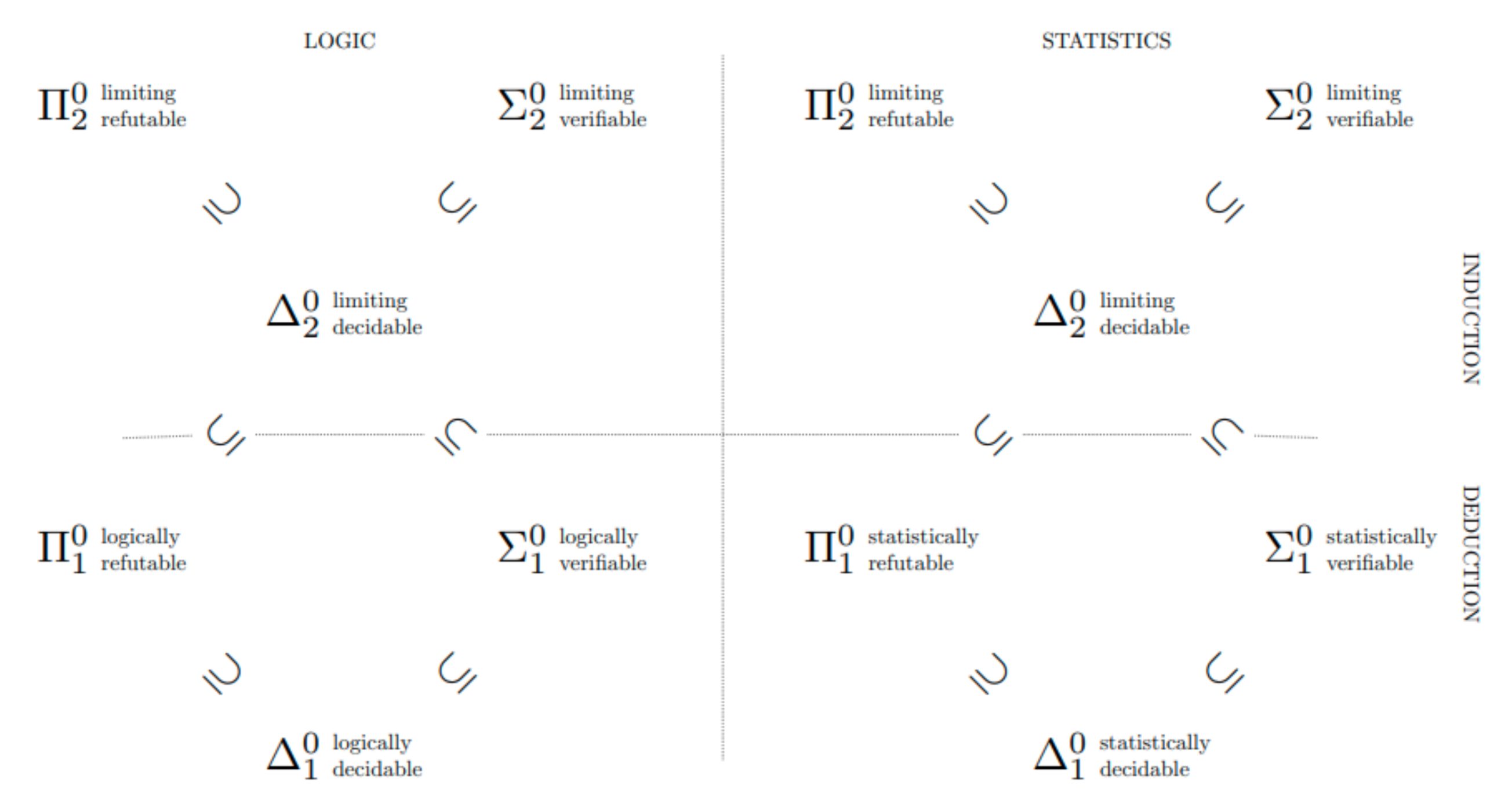
Jointly, C1 and C2 ensure that the collection of all propositions of type F1 constitute the closed sets of a topological space.11 The collection of all propositions of type V1 constitute the open sets of the topology; and the propositions of type D1 constitute the clopen sets of the topology. Sets of greater topological complexity are formed by set-theoretic operations on open and closed sets. The central point of Kelly [30] is that degrees of methodological accessibility correspond exactly to increasingly ramified levels of topological complexity, corresponding to elements of the Borel hierarchy. Roughly speaking, the Borel complexity of a hypothesis measures how complex it is to construct the hypothesis out of logical combinations of verifiable and falsifiable propositions. Higher levels of Borel complexity correspond to inductive notions of methodological success, where by inductive we mean any success notion where the chance of error is unbounded in the short run (see Figure 1).
Taking falsifiability of type F1 as the fundamental notion, the view sketched above was worked out in its essentials by Kelly [30] and further generalized by de Brecht and Yamamoto [31], Genin and Kelly [32] and Baltag et al. [33]. Genin and Kelly [34] exhibit a topology on probability measures in which the closed sets are exactly the propositions falsifiable in the sense of F2. That shows that the structure of statistical verifiability is also topological, at least when issues of monotonicity are ignored. The characteristic asymmetries are all present: while it is possible to falsify that the coin is fair, it is not possible to falsify that it is biased.
In this work, we show that hypotheses of type F3 also enjoy a topological structure; in fact, under a weak assumption, every hypothesis falsifiable in the sense of F2 is also falsifiable in the sense of F3 (Theorem A1). Imposing the demands of monotonicity does not make any fewer hypotheses falsifiable. That result provides a kind of cross-check on our notion of statistical falsifiability: it enjoys the same algebraic closure properties as the traditional notion F1, familiar from classical philosophy of science.
4. The Statistical Setting
4.1. Models, Measures and Samples
A model characterizes the contextually relevant features of a data-generating process. Models may be quite simple, as when they specify the bias of a coin. Models may also be elaborate structural hypotheses, as when they specify a set of structural equations expressing the causal processes by which data are generated. Inquiry typically begins with the specification of a set of possible models , any one of which, for all the inquirers know, may characterize the true data-generating process. Each model determines a probability measure, over a common sample space . A sample space is a set of possible random samples , together with a -algebra of events over the set of samples. Each probability measure is a possible assignments of probabilities to events in that is consistent with the axioms of probability and with the constraints specified by the model . We let W be the set i.e., the set of all probability measures on the sample space generated by possibilities in .
A set of models is said to be identified if the map is one-to-one, i.e., if no two models generate the same probability measure over the space of observable outcomes If two models generate the same probability measure over the observables, then no amount of random sampling can possibly distinguish them and the question of whether or is the generating mechanism is, in a sense, hopeless from a statistical perspective.12 In the following, we will assume that the set of models is identified. Since each probability measure uniquely determines a model, we can identify the model with its probabilistic consequences and drop the subscript from our notation.
Call the triple consisting of a set of probability measures W on a sample space , a statistical setup. The inquirer observes events in , but the hypotheses she is interested in are typically propositions over W. In paradigmatic cases, an event A in is logically consistent with all probability measures in W.
Although measures in W assign probabilities to all events in not all these events are the kinds of events than an agent can observe. No one can tell whether a real-valued sample point is rational or irrational, or if it is exactly For another example, suppose that region A is the closed interval , and that the sample happens to land right on the boundry-point of A. Suppose, furthermore, that given enough time and computational power, the sample can be specified to arbitrary, finite precision. No finite degree of precision: ; ; ; … suffices to determine that is truly in A. But the mere possibility of a sample hitting the boundary of A does not matter statistically, if the chance of obtaining such a sample is zero, as it typically is, unless there is discrete probability mass on the point . Both these examples hinge on an implicit underlying topology on the sample space .
The topology the sample space reflects what is formally verifiable about the sample itself. For example, if is the real line, then it is typically verifiable whether a sample point is greater or less than ; and whether it lies in the interval It is typically not verifiable whether the sample is rational or irrational, or whether it is exactly We assume that these formally verifiable propositions over are closed under finite conjunctions and arbitrary disjunctions and therefore, form the open sets of a topological space. Then, the formally decidable proposition in form the clopen sets of the same topological space. Furthermore, we assume that the -algebra contains all the verifiable proposition and in fact that it is the least such -algebra, i.e., that it is generated by closing the verifiable propositions under countable unions and negations. A -algebra that arises from a topology in this way is called a Borel algebra and its members are called Borel sets.
A Borel set A for which is said to be almost surely clopen (decidable) in μ.13 Say that a collection of Borel sets is almost surely clopen in iff every element of is almost surely clopen in . We say that a Borel set A is almost surely decidable iff it is almost surely decidable in every in W. Similarly, we say that a collection of Borel sets is almost surely clopen iff every element of is almost surely clopen.
A topological basis on is a collection of subsets of such that (1) the elements of cover ; and (2) if are elements of then for each there is containing and contained in Closing a topological basis under unions generates a topology, and every topology is generated by some basis. In the following, we will assume that the topology on is generated by a basis that is at most countably infinite and almost surely clopen. Say that a statistical setup is feasibly based if is a Borel -algebra arising from a countable, almost surely clopen basis. That assumption is satisfied, for example, in the standard case in which the worlds in W are Borel measures on , and all measures are absolutely continuous with respect to Lebesgue measure, i.e., when all measures have probability density functions, which includes normal, chi-square, exponential, Poisson, and beta distributions. It is also satisfied for discrete distributions like the binomial, for which the topology on the sample space is the discrete (power set) topology, so every region in the sample space is clopen. It is satisfied in the particular cases of Examples 1 and 2.
Example 1.
Consider the outcome of a single coin flip. The set Ω of possible outcomes is . Since every outcome is decidable, the appropriate topology on the sample space is , the discrete topology on Ω. Let W be the set of all probability measures assigning a bias to the coin. Since every element of is clopen, every element is also almost surely clopen.
Example 2.
Consider the outcome of a continuous measurement. Then, the sample space Ω is the set of real numbers. Let the basis of the sample space topology be the usual interval basis on the real numbers. That captures the intuition that it is verifiable that the sample landed in some open interval, but it is not verifiable that it landed exactly on the boundary of an open interval. There are no non-trivial decidable (clopen) propositions in that topology. However, in typical statistical applications, W contains only probability measures μ that assign zero probability to the boundary of an arbitrary open interval. Therefore, every open interval E is almost surely decidable, i.e., .
Product spaces represent the outcomes of repeated sampling. Let I be an index set, possibly infinite. Let be sample spaces, each with basis . Define the product of the as follows: let be the Cartesian product of the ; let be the product topology, i.e., the topology in which the open sets are unions of Cartesian products , where each is an element of , and all but finitely many are equal to . When I is finite, the Cartesian products of basis elements in are the intended basis for . Let be the -algebra generated by . Let be a probability measure on , the Borel -algebra generated by the . The product measure is the unique measure on such that, for each expressible as a Cartesian product of , where all but finitely many of the are equal to , . (For a simple proof of the existence of the infinite product measure, see Saeki [37].) Let denote the -fold product of with itself. If W is a set of measures, let denote the set If is a Borel -algebra generated by , let be the Borel -algebra generated by n-fold product of with itself.
4.2. Statistical Tests
A statistical method is a measurable function from random samples to propositions over W, i.e., for every A in the range of its preimage is an element of . A test of a statistical hypothesis is a statistical method . Call the acceptance region, and the rejection region of the test.14 The power of test is the worst-case probability that it rejects truly, i.e., . The significance level of a test is the worst-case probability that it rejects falsely, i.e., .
A test is feasible in μ iff its acceptance region is almost surely decidable in . Say that a test is feasible iff it is feasible in every world in W. More generally, say that a method is feasible iff the preimage of every element of its range is almost surely decidable in every world in W. Tests that are not feasible in are impossible to implement—as described above, if the acceptance region is not almost surely clopen in , then with non-zero probability, the sample lands on the boundary of the acceptance region, where one cannot decide whether to accept or reject. If one were to draw a conclusion at some finite stage, that conclusion might be reversed in light of further computation. Tests are supposed to solve inductive problems, not to generate new ones.
Considerations of feasibility provide a new perspective on the assumption that appears throughout this work: that the basis is almost surely clopen. If that assumption fails, then it is not an a priori matter whether geometrically simple zones are suitable acceptance zones for statistical methods. But if that is not determined a priori, then presumably it must be investigated by statistical means. That suggests a methodological regress in which we must use statistical methods to decide which statistical methods are feasible to use. Therefore, we consider only feasible methods in the following development.
4.3. The Weak Topology
A sequence of measures converges weakly to , written , iff for every A almost surely clopen in . It is immediate that iff for every -feasible test , . It follows that no feasible test of achieves power strictly greater than its significance level. Furthermore, every feasible method that correctly infers H with high chance in , exposes itself to a high chance of error in “nearby” .
It is a standard fact that one can topologize W in such a way that weak convergence is exactly convergence in the topology.15 That topology is called the weak topology, n.b.: the weak topology is a topology on probability measures, whereas all previously mentioned topologies were topologies on random samples. In other words, the open sets of the weak topology are propositions over W, not over If we interpret the closure operator in terms of the weak topology, iff there is a sequence lying in A such that .
If A is an almost surely decidable event in the appropriate -algebra then it is immediate from the definition of weak convergence that and are open in the weak topology over . In this case, it is also true that and are open in the weak topology over W. That observation will often be appealed to in the following. For a proof, see Theorem 2.8 in Billingsley [38].
5. Statistical Falsifiability
Hypothesis H was said to be falsifiable (in the sense of if there is an error avoiding method that converges on increasing information to not-H iff H is false. That condition implies that there is a method that achieves every bound on chance of error, and converges to not-H iff H is false. In statistical settings, one cannot insist on such a high standard of infallibility. Instead, we say that H is falsifiable in chance iff for every bound on error, there is a method that achieves it, and that converges in probability to not-H iff H is false. The reversal of quantifiers expresses the fundamental difference between statistical and propositional falsifiability. The central point in this section is encapsulated in Theorem 1: for feasibly based statistical setups, the statistically falsifiable propositions (in the sense of F2) are exactly the closed sets in the weak topology.
Say that a family of feasible tests of H is an α-falsifier in chance of iff for all :
- BndErr. , if ;
- LimCon. , if .
Say that H is α-falsifiable in chance iff there is an -falsifier in chance of H. Say that H is falsifiable in chance iff H is -falsifiable in chance for every .
Several strengthenings of falsifiability in chance immediately suggest themselves. One could demand that, in addition to BndErr, the chance of error vanishes to zero:
- VanErr. , if .
A strengthening of this requirement will be taken up in the following section.
Defining statistical verifiability requires no new ideas. Say that H is α-verifiable in chance iff there is an -falsifier in chance of . Say that H is verifiable in chance iff is -falsifiable in chance for every .
The central theorem of Genin and Kelly [34] states that, for feasibly based statistical setups, falsifiability in chance is equivalent to being closed in the weak topology.
Theorem 1.
(Fundamental Characterization Theorem). Suppose that the statistical setup is feasibly based. Then, for the following are equivalent:
- H is α-falsifiable in chance for some
- H is falsifiable in chance;
- H is closed in the weak topology on W.
Since a hypothesis is verifiable iff its complement is refutable, the characterization of statistical verifiability follows immediately.
Since a topological space is determined uniquely by its closed sets, Theorem 1 implies that the weak topology is the unique topology that characterizes statistical falsifiability (in the sense of ), at least under the weak conditions stated in the antecedent of the theorem. Thus, under those conditions, the weak topology is not merely a convenient formal tool; it is the fundamental topology for statistical inquiry.
6. Monotonic Falsifiability
In Section 5, we said that is a statistical falsifier of H if it converges to not-H if H is false, and otherwise has a small chance of drawing an erroneous conclusion. But that standard is consistent with a wild see-sawing in the chance of producing the informative conclusion not-H as sample sizes increase, even if H is false. Of course, it is desirable that the chance of correctly rejecting H increases with the sample size, i.e., that for all and ,
- Mon.
Failing to satisfy Mon has the perverse consequence that collecting a larger sample might be a bad idea. Researchers would have to worry whether a failure of replication was due merely to a clumsily designed statistical method that converges to the truth along a needlessly circuitous route. Unfortunately, Mon is infeasible in typical cases, so long as we demand that verifiers satisfy VanErr. Lemma 1 expresses that misfortune.
Say that a statistical setup is purely statistical iff for all and all events such that This is the formal expression of the idea that almost surely clopen sample events have no logical bearing on statistical hypotheses and is easily seen to be a weakening of mutual absolute continuity.
Lemma 1.
Suppose that the statistical setup is feasibly based and purely statistical. Let H be closed, but not open in the weak topology. If is an α-falsifier in chance of H, then, satisfiesVanErronly if it does not satisfy Mon.
Proof of Lemma 1.
Suppose for a contradiction that is an -falsifier in chance of H satisfying VanErr. Since H is not open, there is Since the statistical setup is purely statistical and satisfies LimCon, there must be a sample size such that Let By construction, Since satisfies VanErr, there is such that Let By construction, Since is feasible, both are open in the weak topology (see the observation at the end of Section 4.3). Since open sets are closed under finite conjunction, O is open in the weak topology. But since there is But then, whereas Therefore, does not satisfy Mon. □
But even if strict monotonicity of power is infeasible, it ought to be our regulative ideal. Say that an -falsifier of H, whether in chance, or almost sure, is α-monotonic iff for all and :
- -Mon.
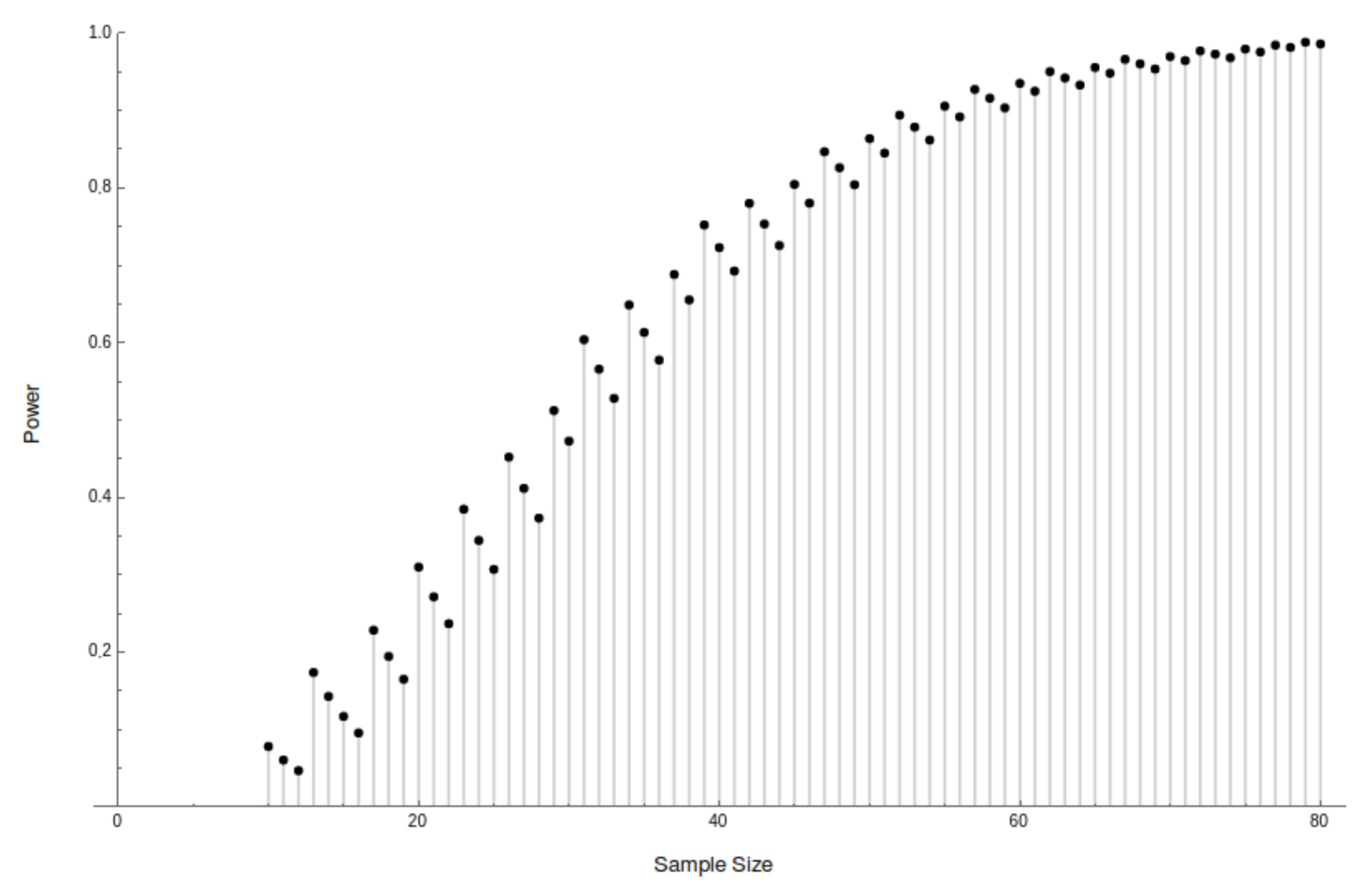
Satisfying -Mon ensures that collecting a larger sample is not a disastrously bad idea. Surprisingly, some standard hypothesis tests fail to satisfy even this weak requirement. Chernick and Liu [23] noticed non-monotonic behavior in the power function of textbook tests of the binomial proportion, and proposed heuristic software solutions. The test exhibited in the Genin and Kelly’s proof of Theorem 1 also displays dramatic non-monotonicity (Figure 2). Others have raised worries of non-monotonicity in consumer safety regulation, vaccine studies, and agronomy [24,25,26].
We now articulate a notion of statistical falsifiability that requires -monotonicity. Write if the sequence converges monotonically to zero. Say that a family of feasible tests of is an α-monotonic falsifier of H iff
- MVanEee. For all , there exists a sequence such that each , and ;
- LimCon., ;
- α-Mon., , if .
Say that H is α-monotonically falsifiable iff there is an -monotonic falsifier of H. Say that H is monotonically falsifiable iff H is -monotonically falsifiable, for every . It is clear that every -monotonic falsifier of H is also an -falsifier in chance. However, not every -monotonic falsifier of H is an almost sure -falsifier. The converse also does not hold.
Defining monotonic verifiability requires no new ideas. Say that H is α-monotonically verifiable in chance iff there is an -monotonic falsifier of . Say that H is montonically verifiable iff is -monotonically refutable for every .
The central theorem of this section states that every statistically falsifiable hypothesis is also monotonically falsifiable. The proof is provided in the Appendix A.
Theorem 2.
Suppose that the statistical setup is feasibly based. Then, for the following are equivalent:
- H is α-falsifiable in chance for some ;
- H is statistically falsifiable;
- H is monotonically falsifiable;
- H is closed in the weak topology on W.
The characterization of monotonic verifiability follows immediately.
7. Conclusions: Falsifiability and Induction
This work is inspired by Popper’s falsificationism and its difficulties with statistical hypotheses. We have proposed several different notions of statistical falsifiability and proven that, whichever definition we prefer, the same hypotheses turn out to be falsifiable. That shows that the notion enjoys a kind of conceptual robustness. Finally, we have demonstrated that, under weak assumptions, the statistically falsifiable hypotheses correspond precisely to the closed sets in a standard topology on probability measures. That means that standard techniques from statistics and measure theory can be used to determine exactly which hypotheses are statistically falsifiable. Hopefully, this result will be a boon to statistical practice by providing a simple diagnostic for statistical falsifiability—controversies about testability may be resolved while maintaining an ecumenical attitude about what, precisely, statistical falsification consists in.
However, this work should not be taken as a wholesale endorsement of Popperian falsificationism. It is easy to generate respectable statistical hypotheses that are not falsifiable or, for that matter, verifiable. Indeed, many pressing scientific hypotheses are of this nature, especially when researchers are interested in answering causal questions (see [39]). These should by no means be regarded as unscientific. The hallmark of these kinds of hypotheses is that, although it is possible to converge to the truth as sample sizes increase, it is not possible to do so with finite sample bounds on the probability of error. This fact should be faced squarely—and not necessarily by searching for stronger assumptions that make it possible to provide finite sample guarantees.
A large class of scientific problems can be reconstructed in the following way: we enumerate a collection of disjoint hypothesis in such a way that that is falsifiable no matter how large n is.16 Then, we test longer and longer initial segments, conjecturing the first hypothesis that we fail to reject. Since the procedure involves nesting tests, we cannot expect finite sample bounds on the probability of conjecturing a false hypothesis. Nevertheless, this procedure answers pretty closely to a Popperian methodology of conjectures and refutations. Unlike Popper, we have no problem calling the outcome of such a procedure—belief in, or acceptance of, the first unrejected hypothesis in the enumeration—an induction. But is there anything to be said in favor of this natural and commonplace scientific procedure? Popper hoped that it would produce theories of greater and greater truthlikeness or verisimilitude. That notion has had a troubled and fascinating career, which we do not review here.17 There is, so far as we know, no demonstration that this procedure must produce theories of increasing truthlikeness.18
Let us briefly consider a different idea. Call such a procedure progressive if (1) it converges in chance to the true (if any is true) and (2) if is true, then the objective chance of conjecturing increases monotonically with sample size. It should come as no surprise that this kind of strict monotonicity is not usually feasible. However, it should be a regulative ideal: say that such a procedure is -progressive if (1’) it converges in chance to the true (if any is true) and (2’) if is true, then the objective chance of conjecturing never decreases by more than as sample sizes increase. The latter is a natural generalization of -Mon to problems of theory choice and precludes egregious backsliding. It should be intuitive that such a procedure can only be -progressive if the constituent test are themselves -monotonic in chance. Genin [45] Theorem 3.6.3, shows that, for all it is possible to produce an -progressive solution to this problem, so long as the consitutent tests are chosen to be sufficiently monotonic in chance. The existence of such tests is guaranteed by Theorem 2. That means that a carefully calibrated methodology of conjectures and refutations is conducive to progress—it converges to the right answer (if any candidate is right) with an arbitrarily low degree of backsliding. We hope that these remarks suggest to some degree the relevance of this work to a positive theory of induction.
Funding
This research was funded by the Deutsche Forschungsgemeinschaft (DFG, German Research Foundation) under Germany’s Excellence Strategy—EXC number 2064/1—Project number 390727645.
Acknowledgments
This work owes a great deal to Kevin Kelly, with whom I had the good fortune of completing my philosophical apprenticeship. I am also grateful to Franz Huber, Conor Mayo-Wilson, Samuel Fletcher, Jonathan Livengood, Kino Zhao and several anonymous reviewers for their generous attention and invaluable input.
Conflicts of Interest
The author declares no conflict of interest.
Appendix A. Proof of Theorem 2
In order to prove Theorem 2, we introduce yet another strengthening of statistical falsifiability. The following strengthens BndErr to the requirement that the total chance of error is bounded:
- σ-BndErr. , if .
That implies both BndErr and VanErr, but also, by the Borel-Cantelli lemma, that with probability one, a verifier makes only finitely many errors on an infinite sample path, whenever H is true:
- SVanErr. if .
We might demand similar asymptotic behavior when H is false. Say that a family of feasible tests of is an almost sure α-falsifer of H iff
- σ-BndErr. , if and
- sLimCon. , if .
Say that H is almost surely α-falsifiable iff there is an almost sure -falsifier of H. Say that H is almost surely falsifiable iff H is almost surely -falsifiable, for every . As usual, we say that H is almost surely verifiable iff its complement is almost surely falsifiable.
Since almost sure convergence entails convergence in chance, almost sure falsifiable entails falsifiability in chance.19
In this section, we prove the following, from which Theorem 2 follows immediately.
Theorem A1.
Suppose that the statistical setup is feasibly based. Then, for the following are equivalent:
- H is α-verifiable in chance for some ;
- H is monotonically verifiable;
- H is almost surely verifiable;
- H is open in the weak topology on W.
In Genin and Kelly [34], it is proven that 1, 3 and 4 are equivalent (see their Theorem 4.1). The fact that 2 implies 1 is immediate from the definitions. To prove that 4 implies 2, we proceed largely as in Genin and Kelly [34], but with greater attention to details.
Recall that a statistical setup is feasibly based if is a Borel -algebra arising from , a countable, almost surely clopen basis. Let be the algebra generated by . Genin and Kelly [34] show that when the statistical setup is feasibly based, the collection of sets of the form where and is a sub-basis for the weak topology. That means that every open set in the weak topology over W can be expressed as a union of finite intersections of elements of the collection. Therefore, we proceed by showing that every element of that collection is monotonically verifiable (Lemma A2). We conclude by showing that the monotonically verifiable propositions are closed under finite intersections (Lemma A3), and countable unions (Lemma A4), which completes the proof. But first, we prove the somewhat technical Lemma A1, which says that if you have a countable collection of -monotonic verifiers , of hypotheses then it is possible to construct a countable collection of mutually independent monotonic verifiers for the . The idea behind the construction is very rudimentary: you can always render methods independent by splitting up the sample in the appropriate way.
Lemma A1.
Suppose that I is a countable index set and that for , is an -monotonic verifier of . Then, there exist where each is an -monotonic verifier of , and for each n, are mutually independent.
Proof of Lemma A1.
The basic idea is to render the mutually independent by splitting the sample and feeding it to the individual verifiers according to a triangular dovetailing scheme. Represented in tabular form:
The samples in the ith column of the table are the samples that are fed to the ith verifier. Since the verifiers are essentially functions of disjoint samples, they are mutually independent. Since the samples are i.i.d. all of the desirable statistical properties of the verifiers are preserved. For a detailed proof, including all the measure-theoretic niceties, see Lemma 3.3.2 in Genin [45]. □
| ⋯ | ||||
| ⋯ | ||||
| ⋮ | ⋮ | ⋮ | ⋮ | ⋯ |
Lemma A2.
Suppose that B is almost surely decidable for every . Then, for all real b, the hypothesis is monotonically verifiable.
Proof of Lemma 2
We restrict attention to the non-trivial cases where . The idea is to take an almost sure -verifier of H and modify it slightly to ensure -monotonicity. See Figure A1 for an overview of the proof strategy. Let and
Genin and Kelly [34] Theorem 4.1, show that is an a.s. -verifier. Let
Then, It is something of a nuisance that is exactly zero for n such that . Since the converge monotonically to 0, this is the case for only finitely many initial sample sizes n. For example, for , is non-trivial for samples sizes larger than 20. Let .
It is worth pointing out some additional features of the that we will be appealing to in the following. It is evident that, since is a polynomial, it is a continuous function of the parameter . Although it is “obviously” true that, for , is strictly increasing in , it is surprisingly non-trivial to demonstrate. For an elegant proof of this fact, see Gilat [46]. It is a standard fact of analysis that that if , are closed real intervals and is a continuous real function, then f is bijective iff it is strictly increasing. Therefore, for , is bijective.
There are two important properties of the collection that follow from the fact that is an almost sure verifier: (1) for , ; (2) . The first property follows from LimCon. The second property follows from -BndErr and the fact that is increasing. Define . Note that for , . Let . For , let
Now, define the increasing step function:
We first show that . If , then . Furthermore, for such that Finally, for such that , .
For , let , for . (The are well defined because is surjective whenever .) Note that since for each i, each . Since for all , there is a least , such that for all , For all n, define to be the least such N. Define and .
We show that . Suppose that Then and . Suppose that for . Then, Finally, suppose that . Then, similarly,
Now, we show that . Suppose that . Then, since, , it follows that , and therefore, Suppose that . Then, . Finally, if , then
It is now easy to show that , since . Therefore, for an increasing sequence of “good” sample sizes, , the verifier is -monotonic. Furthermore, since the sequence converges to zero, there exists a subsequence that converges monotonically to zero. We use these facts to construct a verifier that is -monotonic, by patching over the “bad” sample sizes.
Let . Let We have taken pains to ensure that satisfies -Mon. Since
satisfies MVanErr. Since is an almost sure verifier, the set has for every . But if the sequence converges to H then so does the subsequence . Therefore, . Therefore, , if , and satisfies SLimCon. A fortiori, it also satisfies LimCon. Since was arbitrary, we are done. □
Lemma A3.
The monotonically verifiable propositions are closed under finite conjunctions.
Proof of Lemma A3.
By Lemma A1, it suffices to show that if are mutually independent -monotonic verifiers of , with , then
is an -monotonic verifier of .
Consider the case where . We first demonstrate that satisfies MVanErr. Suppose . Without loss of generality, suppose that . By assumption there exists a sequence such that and . Noticing that
we see that also satisfies MVanErr.
Suppose that . We demonstrate that satisfies LimCon.
But since , it follows that
It remains to show that satisfies -Mon. To make the expressions more manageable, we make the following substitutions:
Under the assumption of independence:
By assumption, either (i) or (ii) . Assume, without loss of generality, that (ii). Then,
The case when follows immediately by induction. □
Lemma A4.
The monotonically verifiable propostions are closed under countable disjunction.
Proof of Lemma A4.
By Lemma A1, it suffices to show that if are mutually independent -monotonic verifiers of such that converges to , then,
is an -monotonic verifier of .
We first demonstrate that satisfies MVanErr. Suppose that . Then, for each i there is such that , , and . Therefore,
It remains to show that converges monotonically to zero as . Since for each i, we have that . Therefore, the sequence is decreasing and bounded below by zero. By the monotone convergence theorem, the sequence converges to its infimum. We show that the infimum is zero. Let . Since the tail of a convergent series tends to zero, there is K such that . Therefore, . Since and as , there is N such that for . Since was arbitrary, we are done.
Suppose that . We show that satisfies LimCon. Since , there is k such that . For
But since , we have that .
It remains to show that satisfies -Mon. By the inclusion-exclusion formula:
To make the expressions more manageable, we make the following substitutions:
Since the verifiers are mutually independent:
Or, in closed form:
Furthermore, for ,
Therefore,
Next, we demonstrate that
By induction on . Let .
Therefore,
Noticing that
where the last equality follows from the inclusion-exclusion principle. It follows that
as required. □
| 1 | Some frequentists go even further. In their response to the American Statistical Association’s controversial statement on p-Values, Ionides et al. [2] identify frequentist method with deduction, and Bayesian method with induction. |
| 2 | Albert [10] answers Redhead’s challenge by suggesting that we drop the fiction that observed variables are continuous. Since we would like our results to apply directly to problems as formulated in the sciences, where continuous variables are commonplace, we do not adopt Albert’s solution. However, we assimilate this insight in Section 4.1 and Section 4.2 by insisting on “feasible” test methods, i.e., methods whose verdicts depend only on a discretization of the data, even if the underlying variables are continuous. |
| 3 | |
| 4 | Kvanvig [15] makes a parallel point for epistemology: “…it is far from obvious that …the best way of structuring a fruitful cognitive life is to concentrate on individual time-slices, and whether knowledge or justification is posessed at each time-slice, and let the totality …get generated by cementing together these time-slices”. Laudan [16] makes a similar point in philosophy of science: “Progress necessarily involves a …process through time. Rationality …has tended to be viewed as an atemporal concept …most writers see progress as nothing more than the temporal projection of individual rational choices …we may be able to learn something by inverting the presumed dependence of progress on rationality”. |
| 5 | We adopt here the idiom of “negative” falsificationism, according to which one should suspend judgement on a hypothesis unless it is falsified. “Positive” falsificationism, on the other hand, endorses belief in hypotheses which have passed an appropriate test (see Musgrave [17], Section 6). If we adopted the positive formulation, we could no longer speak of error avoidance tout court, but would have to rephrase the norm in terms of avoidance of errors of Type I (false rejection). Not much hinges on the choice, since the set of falsififiable hypotheses remains the same. |
| 6 | Here an astute reader may object: how do we know that observation must turn up an elusive non-black raven if one exists? We might rephrase the hypothesis as ‘all ravens that will ever be observed are black.’ We might simply appeal to the background assumptions of inquiry: the method must converge to not-H not in all those possibilities in which H is false, but in all possibilities in which H is false and the background assumptions of inquiry are true. A more careful answer might require a falsification method to converge to not-H in a “maximal set” of possibilities in which H is false, e.g., in all those possibilities in which convergence is compatible with error avoidance. See Liu [18] for a rigorous development of this idea. |
| 7 | The definitions in this section are intentionally rather schematic. Hopefully this will aid, rather than hinder, comprehension. All definitions are formalized in the following. |
| 8 | The reader may object: surely no method can be expected to converge to not-H in all the possibilities in which H is false. For example, what if H is false because the assumption of i.i.d sampling is violated? A more careful formulation requires that the method converge to not-H in all those worlds in which H is false but the background assumptions of inquiry are true—if it is statistical falsification which is at issue, then some kind of statistical regularity must be taken for granted. |
| 9 | The following are only proto-definitions, leaving many things unspecified. The notion of verification in the limit is here a free parameter: compatible notions include convergence in propositional information, convergence in probability and almost sure convergence. The notion of -error avoidance is also parametric: it can mean that the chance of error at any sample size is bounded by , or that the sum of the chances of error over all sample sizes is bounded by . Each of these concepts will be developed in detail in the following. These parametric details are omitted here to expose the essential differences between the three concepts. |
| 10 | For a contrived example, suppose it is known that random samples are distributed uniformly on the interval , for some unknown parameter . Although samples may land outside the interval, they only do so with probability zero. Let H be the hypothesis that the true parameter is . Let M be the method that concludes not-H if some sample lands outside of the interval , and draws no non-trivial conclusion otherwise. Then, M is a deductive falsifier of the second type, although not of the first. Clearly, every falsifier of the first type is a falsifier of the second type. |
| 11 | A topological space is a structure where W is a set, and is a collection of subsets of W closed under conjunction and finite disjunction. The elements of are called the closed sets of . In our case W is a set of epistemic possibilities, or possible worlds, and is the set of falsifiable propositions over W. Although we define a topology here in terms of closed sets, we could just as easily have done it in terms of open sets since the complement of every closed set is open. |
| 12 | |
| 13 | We use the notation to denote the set of boundary points of A. |
| 14 | The acceptance region is , rather than , because failing to reject H licenses only suspension of belief i.e., the trivial inference W. |
| 15 | Every topology gives rise to a kind of convergence by setting iff for every open E containing there is N such that for . Every kind of convergence gives rise to a topology by letting be open iff for each sequence there is N such that for . The notion of convergence arising from a topology defined in this way will agree with the original notion of convergence. |
| 16 | For example, if we are interpolating points with polynomials, linear, quadratic, cubic, ... is such a collection, when the hypotheses are understood in the strict sense. Although the individual hypotheses are not falsifiable—if the truth is linear, quadratic will never be refuted—unions of inital segments are—if the generating polynomial is of degree greater than 2, we will get a sign. Many statistical model selection problems also fit this description. |
| 17 | |
| 18 | Niiniluoto [43] admits: “the problem of estimating verisimilitude is neither more nor less difficult than the traditional problem of induction”. |
| 19 | This entailment holds only for countably additive measures, to which we restrict attention. |
References
- Gelman, A.; Shalizi, C.R. Philosophy and the practice of Bayesian statistics. Br. J. Math. Stat. Psychol. 2013, 66, 8–38. [Google Scholar] [CrossRef] [PubMed] [Green Version]
- Ionides, E.L.; Giessing, A.; Ritov, Y.; Page, S.E. Response to the ASA’s Statement on p-Values: Context, Process, and Purpose. Am. Stat. 2017, 71, 88–89. [Google Scholar] [CrossRef]
- Popper, K.R. The Logic of Scientific Discovery, 1st ed.; Hutchinson: London, UK, 1959. [Google Scholar]
- Gillies, D.A. A Falsifying Rule for Probability Statements. Br. J. Philos. Sci. 1971, 22, 231–261. [Google Scholar] [CrossRef]
- Albert, M. Die Falsifikation Statistischer Hypothesen. J. Gen. Philos. Sci. 1992, 23, 1–32. [Google Scholar] [CrossRef]
- Mayo, D.G.; Spanos, A. Severe testing as a basic concept in a Neyman–Pearson philosophy of induction. Br. J. Philos. Sci. 2006, 57, 323–357. [Google Scholar]
- Fisher, R.A. Statistical Methods and Scientific Inference; Oliver and Boyd: Edinburgh, UK, 1959. [Google Scholar]
- Neyman, J. Lectures and Conferences on Mathematical Statistics and Probability; Graduate School, US Department of Agriculture: Washington, DC, USA, 1952.
- Redhead, M. On Neyman’s paradox and the theory of statistical tests. Br. J. Philos. Sci. 1974, 25, 265–271. [Google Scholar]
- Albert, M. Resolving Neyman’s Paradox. Br. J. Philos. Sci. 2020, 53, 69–76. [Google Scholar] [CrossRef]
- Neyman, J.; Pearson, E.S. IX. On the problem of the most efficient tests of statistical hypotheses. Philos. Trans. R. Soc. Lond. Ser. A Contain. Pap. Math. Phys. Character 1933, 231, 289–337. [Google Scholar]
- Casella, G.; Berger, R.L. Statistical Inference, 2nd ed.; Duxbury: Pacific Grove, CA, USA, 2002. [Google Scholar]
- Shah, R.D.; Peters, J. The hardness of conditional independence testing and the generalised covariance measure. Ann. Stat. 2020, 48, 1514–1538. [Google Scholar]
- Neykov, M.; Balakrishnan, S.; Wasserman, L. Minimax optimal conditional independence testing. Ann. Stat. 2021, 49, 2151–2177. [Google Scholar]
- Kvanvig, J.L. The Intellectual Virtues and the Life of the Mind: On the Place of Virtues in Contemporary Epistemology; Rowman and Littlefield: Savage, MD, USA, 1992. [Google Scholar]
- Laudan, L. Progress and its Problems: Towards a Theory of Scientific Growth; University of California Press: Berkeley, CA, USA, 1978. [Google Scholar]
- Musgrave, A. Critical Rationalism. In The Power of Argumentation; Poznań Studies in the Philosophy of the Sciences and the, Humanities; Suárez-Iñiguez, E., Ed.; Brill: Leiden, The Netherlands, 2007; pp. 171–211. [Google Scholar]
- Lin, H. Modes of convergence to the truth: Steps toward a better epistemology of induction. Rev. Symb. Log. 2022, forthcoming. [Google Scholar]
- Bar-Hillel, Y.; Carnap, R. Semantic Information. Br. J. Philos. Sci. 1953, 4, 147–157. [Google Scholar]
- Floridi, L. Is semantic information meaningful data? Philos. Phenomenol. Res. 2005, 70, 351–370. [Google Scholar] [CrossRef] [Green Version]
- Floridi, L. The Philosophy of Information; Oxford University Press: Oxford, UK, 2011. [Google Scholar]
- Niranjan, S.; Frenzel, J.F. A comparison of fault-tolerant state machine architectures for space-borne electronics. IEEE Trans. Reliab. 1996, 45, 109–113. [Google Scholar] [CrossRef]
- Chernick, M.R.; Liu, C.Y. The saw-toothed behavior of power versus sample size and software solutions: Single binomial proportion using exact methods. Am. Stat. 2002, 56, 149–155. [Google Scholar] [CrossRef]
- Schuette, P.; Rochester, C.G.; Jackson, M. Power and sample size for safety registries: New methods using confidence intervals and saw-tooth power curves. In Proceedings of the 8th International R User Conference, Nashville, TN, USA, 12–15 June 2012. [Google Scholar]
- Musonda, P. The Self-Controlled Case Series Method: Performance and Design in Studies of Vaccine Safety. Ph.D. Thesis, Open University, Milton Keynes, UK, 2006. [Google Scholar]
- Schaarschmidt, F. Experimental design for one-sided confidence intervals or hypothesis tests in binomial group testing. Commun. Biometry Crop. Sci. 2007, 2, 32–40. [Google Scholar]
- Genin, K.; Mayo-Wilson, C. Statistical Decidability in Linear, Non-Gaussian Causal Models. In Proceedings of the Causal Discovery & Causality-Inspired Machine Learning Workshop, NeurIPS, Virtual, 11–12 December 2020. [Google Scholar]
- Abramsky, S. Domain Theory and the Logic of Observable Properties. Ph.D. Thesis, University of London, London, UK, 1987. [Google Scholar]
- Vickers, S. Topology Via Logic; Cambridge University Press: Cambridge, UK, 1996. [Google Scholar]
- Kelly, K.T. The Logic of Reliable Inquiry; Oxford University Press: Oxford, UK, 1996. [Google Scholar]
- de Brecht, M.; Yamamoto, A. Interpreting learners as realizers for ()-measurable functions. Spec. Interes. Group Fundam. Probl. Artif. Intell. (SIG-FPAI) 2009, 74, 39–44. [Google Scholar]
- Genin, K.; Kelly, K.T. Theory Choice, Theory Change, and Inductive Truth-Conduciveness. In Proceedings of the Fifteenth Conference on Theoretical Aspects of Rationality and Knowledge (TARK), Pittsburgh, PA, USA, 4–6 June 2015; pp. 111–121. [Google Scholar]
- Baltag, A.; Gierasimczuk, N.; Smets, S. On the Solvability of Inductive Problems: A Study in Epistemic Topology. Electron. Proc. Theor. Comput. Sci. 2016, 215, 81–98. [Google Scholar] [CrossRef] [Green Version]
- Genin, K.; Kelly, K.T. The Topology of Statistical Verifiability. In Proceedings of the Sixteenth Conference on Theoretical Aspects of Rationality and Knowledge (TARK), Liverpool, UK, 24–26 July 2017; pp. 236–250. [Google Scholar] [CrossRef] [Green Version]
- Lin, H. The Hard Problem of Theory Choice: A Case Study on Causal Inference and Its Faithfulness Assumption. Philos. Sci. 2019, 86, 967–980. [Google Scholar]
- Lin, H.; Zhang, J. On Learning Causal Structures from Non-Experimental Data without Any Faithfulness Assumption. In Proceedings of the Algorithmic Learning Theory, PMLR, San Diego, CA, USA, 8–11 February 2020; pp. 554–582. [Google Scholar]
- Saeki, S. A proof of the existence of infinite product probability measures. Am. Math. Mon. 1996, 103, 682–683. [Google Scholar] [CrossRef]
- Billingsley, P. Convergence of Probability Measures, 2nd ed.; John Wiley & Sons: Hoboken, NJ, USA, 1999. [Google Scholar] [CrossRef] [Green Version]
- Genin, K. Statistical Undecidability in Linear, Non-Gaussian Models in the Presence of Latent Confounders. In Proceedings of the Advances in Neural Information Processing Systems 34, Virtual, 6–12 December 2020. [Google Scholar]
- Miller, D. Popper’s qualitative theory of verisimilitude. Br. J. Philos. Sci. 1974, 25, 166–177. [Google Scholar] [CrossRef]
- Tichý, P. On Popper’s definitions of verisimilitude. Br. J. Philos. Sci. 1974, 25, 155–160. [Google Scholar] [CrossRef]
- Oddie, G. Likeness to Truth; The University of Western Ontario Series in Philosoph of Science; Reidel: Dordrecht, The Netherlands, 1986; Volume 30. [Google Scholar]
- Niiniluoto, I. Truthlikeness; The Synthese Library; Reidel: Dordrecht, The Netherlands, 1987; Volume 185. [Google Scholar]
- Niiniluoto, I. Critical Scientific Realism; Oxford University Press: Oxford, UK, 1999. [Google Scholar]
- Genin, K. The Topology of Statistical Inquiry. Ph.D. Thesis, Carnegie Mellon University, Pittsburgh, PA, USA, 2018. [Google Scholar]
- Gilat, D. Monotonicity of a power function: An elementary probabilistic proof. Am. Stat. 1977, 31, 91–93. [Google Scholar] [CrossRef]
Figure 1.
Pictured is a hierarchy of topological complexity and corresponding notions of methodological success. The set of all open sets is referred to as ; the set of all closed sets as ; and the set of all clopen sets as . Depending on whether the sets are propositions of type V1 or V2, we get the logical (left) and statistical (right) hierarchies. Sets of greater complexity are built out of sets by logical operations, e.g., sets are countable unions of locally closed sets. Inclusion relations between notions of complexity are also indicated. For more on the notions of methodological success characterized by higher levels of Borel complexity, see Genin and Kelly [34].

Figure 2.
Diachronic plot of power of typical test of the null hypothesis that a coin is not head-biased, when p(H) = 0.775. The plot exhibits the characteristic “saw-tooth” shape identified by Chernick and Liu [23]. Note that the drops in power are significant e.g., >0.07 between sample sizes 31 and 33.

Figure A1.
The basic idea of the proof is encapsulated in the figure. For any sample size n, we construct a step function that “almost dominates” the power function The step function dominates for all except those for which is less than , or close to 1. Then, since the set of steps is finite, and the original test satisfies LimCon, there must be a sample size such that the power function strictly dominates the step function. Since dominates the step function, can only be less than if is less than or they are both close to 1. The loss of power from n to is thereby bounded by Iterating this process we get a sequence of “good” sample sizes such that the power is “almost increasing”. It remains only to interpolate the intermediate sample sizes with tests that throw out samples until they arrive at the nearest “good” sample size.

Publisher’s Note: MDPI stays neutral with regard to jurisdictional claims in published maps and institutional affiliations. |
© 2022 by the author. Licensee MDPI, Basel, Switzerland. This article is an open access article distributed under the terms and conditions of the Creative Commons Attribution (CC BY) license (https://creativecommons.org/licenses/by/4.0/).
Share and Cite
MDPI and ACS Style
Genin, K. On Falsifiable Statistical Hypotheses. Philosophies 2022, 7, 40. https://doi.org/10.3390/philosophies7020040
AMA Style
Genin K. On Falsifiable Statistical Hypotheses. Philosophies. 2022; 7(2):40. https://doi.org/10.3390/philosophies7020040
Chicago/Turabian StyleGenin, Konstantin. 2022. "On Falsifiable Statistical Hypotheses" Philosophies 7, no. 2: 40. https://doi.org/10.3390/philosophies7020040