
Distributed State Estimation for Flapping-Wing Micro Air Vehicles with Information Fusion Correction


Abstract
:1. Introduction
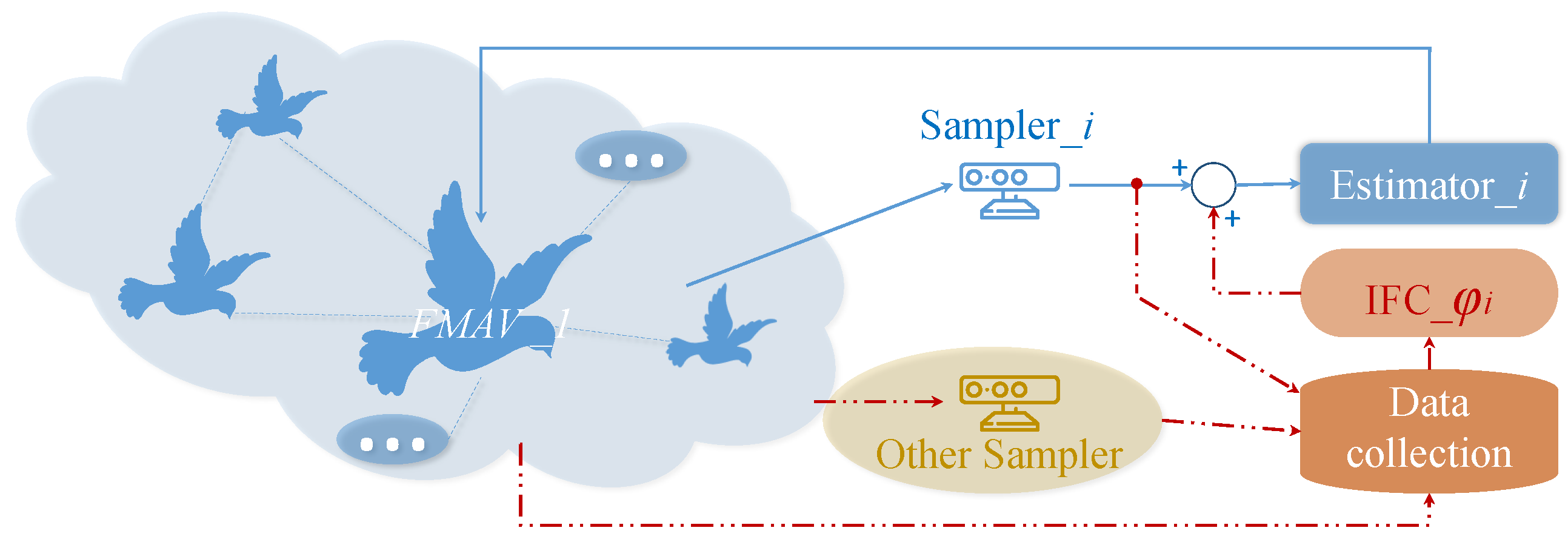
- Improving the traditional distributed state estimator and introducing information fusion correction between nodes in the FMAV network system to enhance estimation accuracy.
- Equipping each FMAV with an independent sampler, featuring variable sampling periods and utilizing a time delay study method to transform the state estimation problem based on non-uniform sampling into a problem with multiple bounded time delays.
- Constructing the LKF by fully exploiting time delay information induced by non-uniform sampling. This approach avoids the introduction of complex multiple integrals and generalized functions, effectively reducing the computational burden.
- Proposing an easy-to-implement distributed state estimation method with minimal conservatism by employing relaxed and Wirtinger integral inequalities in deflating generalized functions.
2. Problem Formulation
- The estimated error system is asymptotically stable in the case of and ;
- With zero-initial condition, for all nonzero and , the output estimation error satisfieswhere is a prescribed disturbance attenuation level.
3. Main Results
4. Simulations
5. Conclusions
Author Contributions
Funding
Institutional Review Board Statement
Data Availability Statement
Conflicts of Interest
References
- Fang, X.; Wen, Y.; Gao, Z.; Gao, K.; Luo, Q.; Peng, H.; Du, R. Review of the Flight Control Method of a Bird-like Flapping-Wing Air Vehicle. Micromachines 2023, 14, 1547. [Google Scholar] [CrossRef]
- Orlowski, C.T.; Girard, A.R. Dynamics, stability, and control analyses of flapping wing micro-air vehicles. Prog. Aerosp. Sci. 2012, 51, 18–30. [Google Scholar] [CrossRef]
- Gerdes, J.W.; Gupta, S.K.; Wilkerson, S.A. A review of bird-inspired flapping wing miniature air vehicle designs. J. Mech. Robot. 2012, 4, 021003. [Google Scholar] [CrossRef]
- Hassanalian, M.; Abdelkefi, A.; Wei, M.; Ziaei-Rad, S. A novel methodology for wing sizing of bio-inspired flapping wing micro air vehicles: Theory and prototype. Acta Mech. 2017, 228, 1097–1113. [Google Scholar] [CrossRef]
- Anderson, M.L. Design and Control of Flapping Wing Micro Air Vehicles. Ph.D. Thesis, Air Force Institute of Technology, Dayton, OH, USA, 2011. [Google Scholar]
- Bhatti, M.Y.; Lee, S.G.; Han, J.H. Dynamic Stability and Flight Control of Biomimetic Flapping-Wing Micro Air Vehicle. Aerospace 2021, 8, 362. [Google Scholar] [CrossRef]
- Keennon, M.; Klingebiel, K.; Won, H. Development of the nano hummingbird: A tailless flapping wing micro air vehicle. In Proceedings of the 50th AIAA Aerospace Sciences Meeting Including the New Horizons Forum and Aerospace Exposition, Nashville, TN, USA, 9–12 January 2012; p. 588. [Google Scholar]
- Send, W.; Fischer, M.; Jebens, K.; Mugrauer, R.; Nagarathinam, A.; Scharstein, F. Artificial hinged-wing bird with active torsion and partially linear kinematics. In Proceedings of the 28th Congress of the International Council of the Aeronautical Sciences, Brisbane, Australia, 23–28 September 2012; Volume 10. [Google Scholar]
- Yang, W.; Wang, L.; Song, B. Dove: A biomimetic flapping-wing micro air vehicle. Int. J. Micro Air Veh. 2018, 10, 70–84. [Google Scholar] [CrossRef]
- Doman, D.B.; Oppenheimer, M.W.; Sigthorsson, D.O. Wingbeat shape modulation for flapping-wing micro-air-vehicle control during hover. J. Guid. Control. Dyn. 2010, 33, 724–739. [Google Scholar] [CrossRef]
- Khosravi, M.; Novinzadeh, A. A multi-body control approach for flapping wing micro aerial vehicles. Aerosp. Sci. Technol. 2021, 112, 106525. [Google Scholar] [CrossRef]
- Jeong, S.H.; Kim, J.H.; Choi, S.I.; Park, J.K.; Kang, T.S. Platform Design and Preliminary Test Result of an Insect-like Flapping MAV with Direct Motor-Driven Resonant Wings Utilizing Extension Springs. Biomimetics 2022, 8, 6. [Google Scholar] [CrossRef]
- Xue, D.; Song, B.; Song, W. Longitudinal Trim and Dynamic Stability Analysis of a Seagull-Based Model. Appl. Sci. 2022, 12, 5440. [Google Scholar] [CrossRef]
- Billingsley, E.; Ghommem, M.; Vasconcellos, R.; Abdelkefi, A. On the aerodynamic analysis and conceptual design of bioinspired multi-flapping-wing drones. Drones 2021, 5, 64. [Google Scholar] [CrossRef]
- Wang, Z.; Shen, B.; Liu, X. H∞ filtering with randomly occurring sensor saturations and missing measurements. Automatica 2012, 48, 556–562. [Google Scholar] [CrossRef]
- Qian, W.; Zhang, X.; Zhao, Y.; Zhang, X. Distributed H∞ state estimation in sensor network subject to state and communication delays. Circuits Syst. Signal Process. 2021, 40, 3227–3243. [Google Scholar] [CrossRef]
- Widhiarini, S.; Park, J.H.; Yoon, B.S.; Yoon, K.J.; Paik, I.H.; Kim, J.H.; Park, C.Y.; Jun, S.M.; Nam, C. Bird-mimetic wing system of flapping-wing micro air vehicle with autonomous flight control capability. J. Bionic Eng. 2016, 13, 458–467. [Google Scholar] [CrossRef]
- Noda, R.; Nakata, T.; Liu, H. Effect of Hindwings on the Aerodynamics and Passive Dynamic Stability of a Hovering Hawkmoth. Biomimetics 2023, 8, 578. [Google Scholar] [CrossRef] [PubMed]
- Xue, Y.; Cai, X.; Xu, R.; Liu, H. Wing Kinematics-Based Flight Control Strategy in Insect-Inspired Flight Systems: Deep Reinforcement Learning Gives Solutions and Inspires Controller Design in Flapping MAVs. Biomimetics 2023, 8, 295. [Google Scholar] [CrossRef] [PubMed]
- Mousavi, S.M.; Pourtakdoust, S.H. Improved Neural Adaptive Control for Nonlinear Oscillatory Dynamic of Flapping Wings. J. Guid. Control. Dyn. 2023, 46, 97–113. [Google Scholar] [CrossRef]
- Liu, G.; Wang, S.; Xu, W. Flying State Sensing and Estimation Method of Large-Scale Bionic Flapping Wing Flying Robot. Actuators 2022, 11, 213. [Google Scholar] [CrossRef]
- Yang, R.; Zhang, W.; Mou, J.; Zhang, B.; Zhang, Y. Attitude Estimation Algorithm of Flapping-Wing Micro Air Vehicle Based on Extended Kalman Filter. In Proceedings of the International Conference on Autonomous Unmanned Systems, Xi’an, China, 23–25 September 2022; pp. 1432–1443. [Google Scholar]
- He, W.; Yan, Z.; Sun, C.; Chen, Y. Adaptive neural network control of a flapping wing micro aerial vehicle with disturbance observer. IEEE Trans. Cybern. 2017, 47, 3452–3465. [Google Scholar] [CrossRef] [PubMed]
- Qian, W.; Lu, D.; Guo, S.; Zhao, Y. Distributed state estimation for mixed delays system over sensor networks with multichannel random attacks and Markov switching topology. In IEEE Transactions on Neural Networks and Learning Systems; IEEE: New York, NY, USA, 2022. [Google Scholar]
- Hu, Z.; Hu, J.; Yang, G. A survey on distributed filtering, estimation and fusion for nonlinear systems with communication constraints: New advances and prospects. Syst. Sci. Control Eng. 2020, 8, 189–205. [Google Scholar] [CrossRef]
- Pizá, R.; Carbonell, R.; Casanova, V.; Cuenca, Á.; Salt Llobregat, J.J. Nonuniform dual-rate extended kalman-filter-based sensor fusion for path-following control of a holonomic mobile robot with four mecanum wheels. Appl. Sci. 2022, 12, 3560. [Google Scholar] [CrossRef]
- Fridman, E.; Seuret, A.; Richard, J.P. Robust sampled-data stabilization of linear systems: An input delay approach. Automatica 2004, 40, 1441–1446. [Google Scholar] [CrossRef]
- Wang, L.; Wang, Z.; Wei, G.; Alsaadi, F.E. Variance-constrained H∞ state estimation for time-varying multi-rate systems with redundant channels: The finite-horizon case. Inf. Sci. 2019, 501, 222–235. [Google Scholar] [CrossRef]
- Lin, H.; Sun, S. Globally optimal sequential and distributed fusion state estimation for multi-sensor systems with cross-correlated noises. Automatica 2019, 101, 128–137. [Google Scholar] [CrossRef]
- Li, Q.; Shen, B.; Wang, Z.; Alsaadi, F.E. A sampled-data approach to distributed H∞ resilient state estimation for a class of nonlinear time-delay systems over sensor networks. J. Frankl. Inst. 2017, 354, 7139–7157. [Google Scholar] [CrossRef]
- Sun, D.; Xing, S.; Li, Y.; Pang, B.; Wang, X. Sub-aperture partitioning method for three-dimensional wide-angle synthetic aperture radar imaging with non-uniform sampling. Electronics 2019, 8, 629. [Google Scholar] [CrossRef]
- Wang, J.; Han, L.; Li, X.; Dong, X.; Li, Q.; Ren, Z. Time-varying formation of second-order discrete-time multi-agent systems under non-uniform communication delays and switching topology with application to UAV formation flying. IET Control Theory Appl. 2020, 14, 1947–1956. [Google Scholar] [CrossRef]
- Yang, B.; Cao, J.; Hao, M.; Pan, X. Further stability analysis of generalized neural networks with time-varying delays based on a novel Lyapunov-Krasovskii functional. IEEE Access 2019, 7, 91253–91264. [Google Scholar] [CrossRef]
- Zeng, H.B.; Liu, X.G.; Wang, W. A generalized free-matrix-based integral inequality for stability analysis of time-varying delay systems. Appl. Math. Comput. 2019, 354, 1–8. [Google Scholar] [CrossRef]
- Dong, H.; Wang, Z.; Lam, J.; Gao, H. Distributed filtering in sensor networks with randomly occurring saturations and successive packet dropouts. Int. J. Robust Nonlinear Control 2014, 24, 1743–1759. [Google Scholar] [CrossRef]
- Park, P.G.; Lee, W.I.; Lee, S.Y. Auxiliary Function-based Integral Inequalities for Quadratic Functions and their Applications to Time-delay Systems. J. Frankl. Inst. 2015, 352, 1378–1396. [Google Scholar] [CrossRef]
- Liu, K.; Seuret, A. Comparison of bounding methods for stability analysis of systems with time-varying delays. J. Frankl. Inst. 2017, 354, 2979–2993. [Google Scholar] [CrossRef]


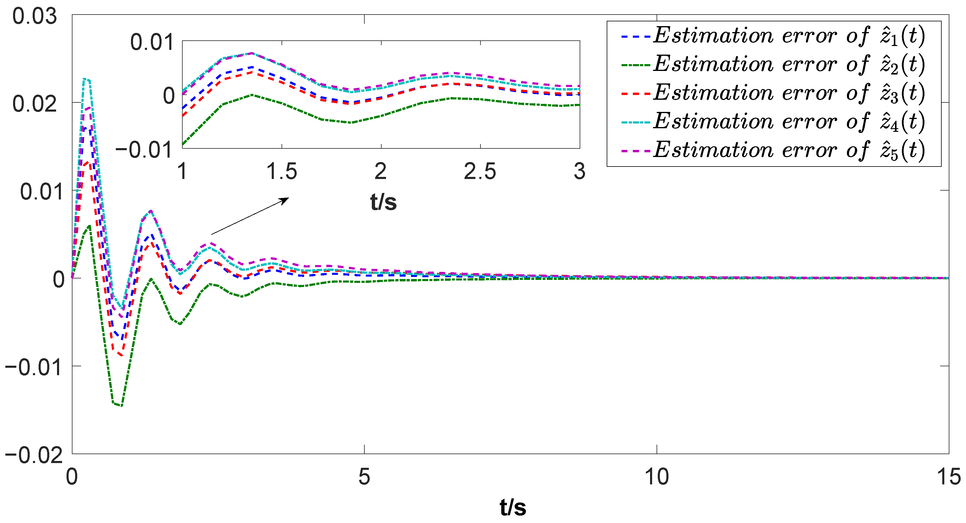
| 0.017 | 0.006 | 0.013 | 0.023 | 0.019 | |
| −0.007 | −0.015 | −0.009 | −0.003 | −0.004 | |
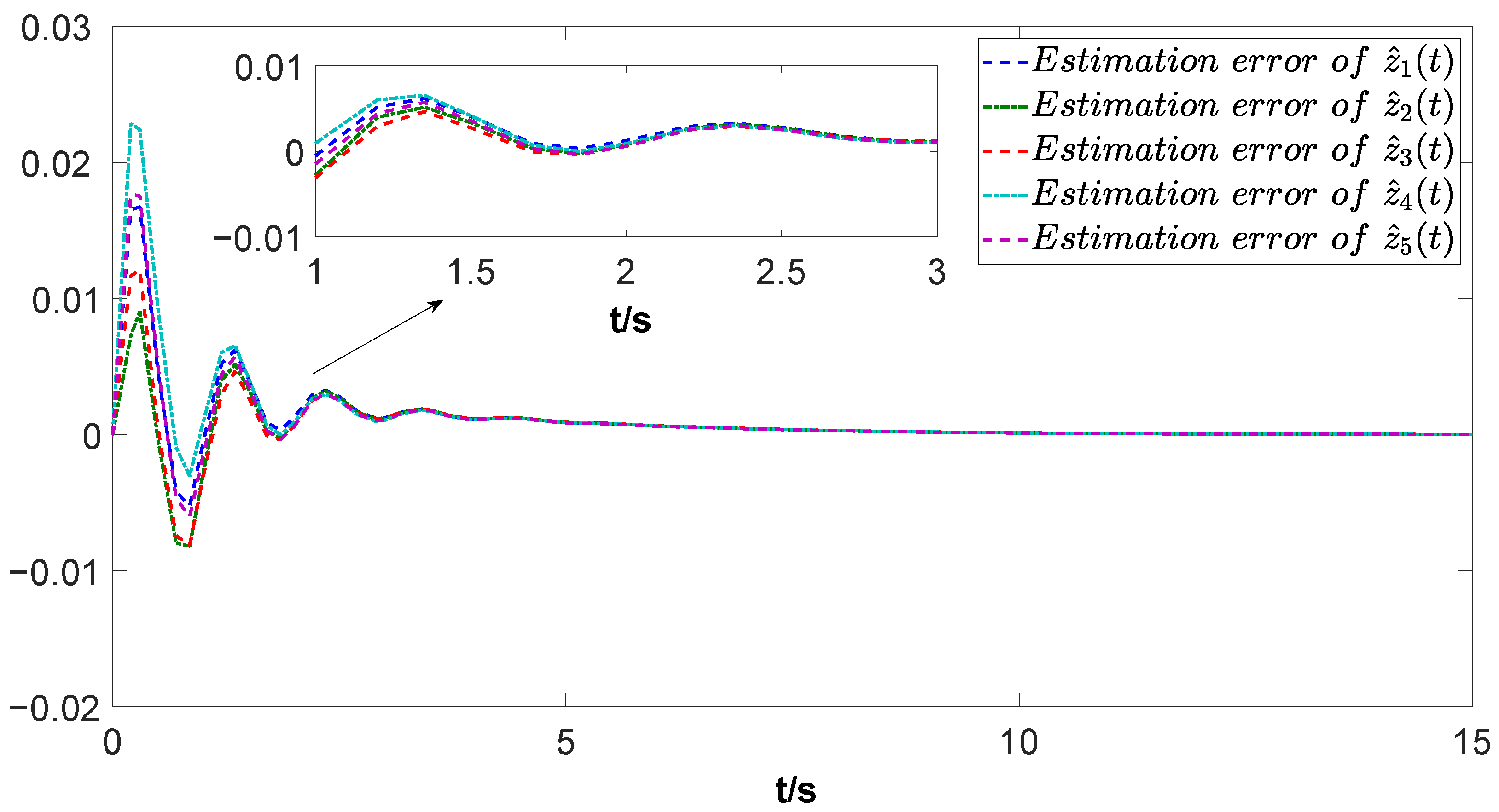
| 0.017 | 0.009 | 0.012 | 0.023 | 0.018 | |
| −0.005 | −0.008 | −0.008 | −0.003 | −0.006 |
Disclaimer/Publisher’s Note: The statements, opinions and data contained in all publications are solely those of the individual author(s) and contributor(s) and not of MDPI and/or the editor(s). MDPI and/or the editor(s) disclaim responsibility for any injury to people or property resulting from any ideas, methods, instructions or products referred to in the content. |
© 2024 by the authors. Licensee MDPI, Basel, Switzerland. This article is an open access article distributed under the terms and conditions of the Creative Commons Attribution (CC BY) license (https://creativecommons.org/licenses/by/4.0/).
Share and Cite
Zhang, X.; Luo, M.; Guo, S.; Cui, Z. Distributed State Estimation for Flapping-Wing Micro Air Vehicles with Information Fusion Correction. Biomimetics 2024, 9, 167. https://doi.org/10.3390/biomimetics9030167
Zhang X, Luo M, Guo S, Cui Z. Distributed State Estimation for Flapping-Wing Micro Air Vehicles with Information Fusion Correction. Biomimetics. 2024; 9(3):167. https://doi.org/10.3390/biomimetics9030167
Chicago/Turabian StyleZhang, Xianglin, Mingqiang Luo, Simeng Guo, and Zhiyang Cui. 2024. "Distributed State Estimation for Flapping-Wing Micro Air Vehicles with Information Fusion Correction" Biomimetics 9, no. 3: 167. https://doi.org/10.3390/biomimetics9030167