
An Enhanced Hunger Games Search Optimization with Application to Constrained Engineering Optimization Problems


Abstract
:1. Introduction
- The introduced strategy enhance the exploration and exploitation process of ordinary HGS algorithms when solving optimization problems.
- To evaluate the efficacy of the proposed approach, RLHGS is compared with eight other state-of-the-art algorithms on 23 classical benchmark functions and 10 benchmark functions from CEC2020. And the comparative evaluation of these experiments demonstrates the superiority of RLHGS in terms of optimization performance.
- The proposed RLHGS algorithm addresses four constrained real-world problems, showcasing its practical applicability and effectiveness in tackling complex engineering challenges.
- The experiment results of RLHGS indicate excellent accuracy and reliable performance.
2. Preliminaries
2.1. Description of Hunger Games Search
2.1.1. Approach Food
2.1.2. Hunger Role
| Algorithm 1: Pseudo-code of HGS. |
| Initialize the parameters N, T, l, D, Sum_hungry |
| Initialize the population |
| While |
| Calculate the initial fitness of all populations |
| Update BF, WF, and Xb |
| Calculate hungry by using Equation (8) |
| Calculate W1 and W2 by using Equations (6) and (7), respectively |
| For i = 1 to N |
| If (rand < 0.3) |
| Update the position of the current search agent by using Equation (1) |
| Else |
| Calculate E by using Equation (2) |
| Update R using Equation (4) |
| Update the position of the current search agent by Equation (1) |
| End if |
| End For |
| t = t + 1 |
| End While |
| Return BF and Xb |
2.2. The Adapted Logarithmic Spiral Strategy
2.3. The Adapted Rosenbrock Method Strategy
| Algorithm 2: Pseudo-code of the adapted RM strategy. |
| Input . |
| . |
| . |
| While)) |
| ) |
| ) |
| Else |
| End If |
| End for |
| Else |
| End If |
| End While |
| ) |
| Update the orthonormal basis . |
| End If |
| End While |
| Return |
3. Description of Proposed RLHGS
3.1. Motivation for This Work
3.2. Flowchart and Pseudo-Code of RLHGS
| Algorithm 3: Pseudo-code of RLHGS. |
| While ) |
| Calculate the initial fitness of all populations |
| by using Equation (8) |
| by using Equations (6) and (7), respectively |
| For |
| If ( < 0.3) |
| Update the position of the current search agent by using the adapted LS-OBL strategy |
| Else |
| by using Equation (2) |
| Update using Equation (4) |
| Update the position of the current search agent by Equation (1) |
| If ( > 0.8) |
| Update the position of the current search agent by using the adapted RM strategy |
| End If |
| End If |
| End For |
| + 1 |
| End While |
| Return |
3.3. Computational Complexity Analysis
4. Designs for Experiments
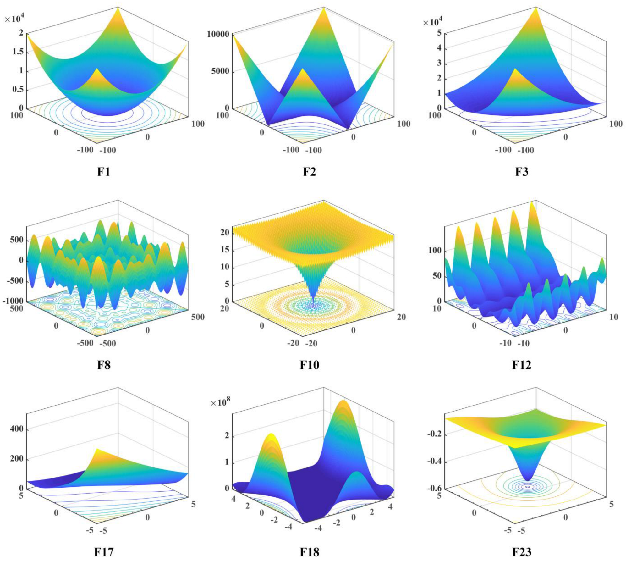
4.1. Details of Benchmark Functions
4.2. Configuration of Experiment Environment
4.3. Statistical Analysis Methods
5. Result and Discussion
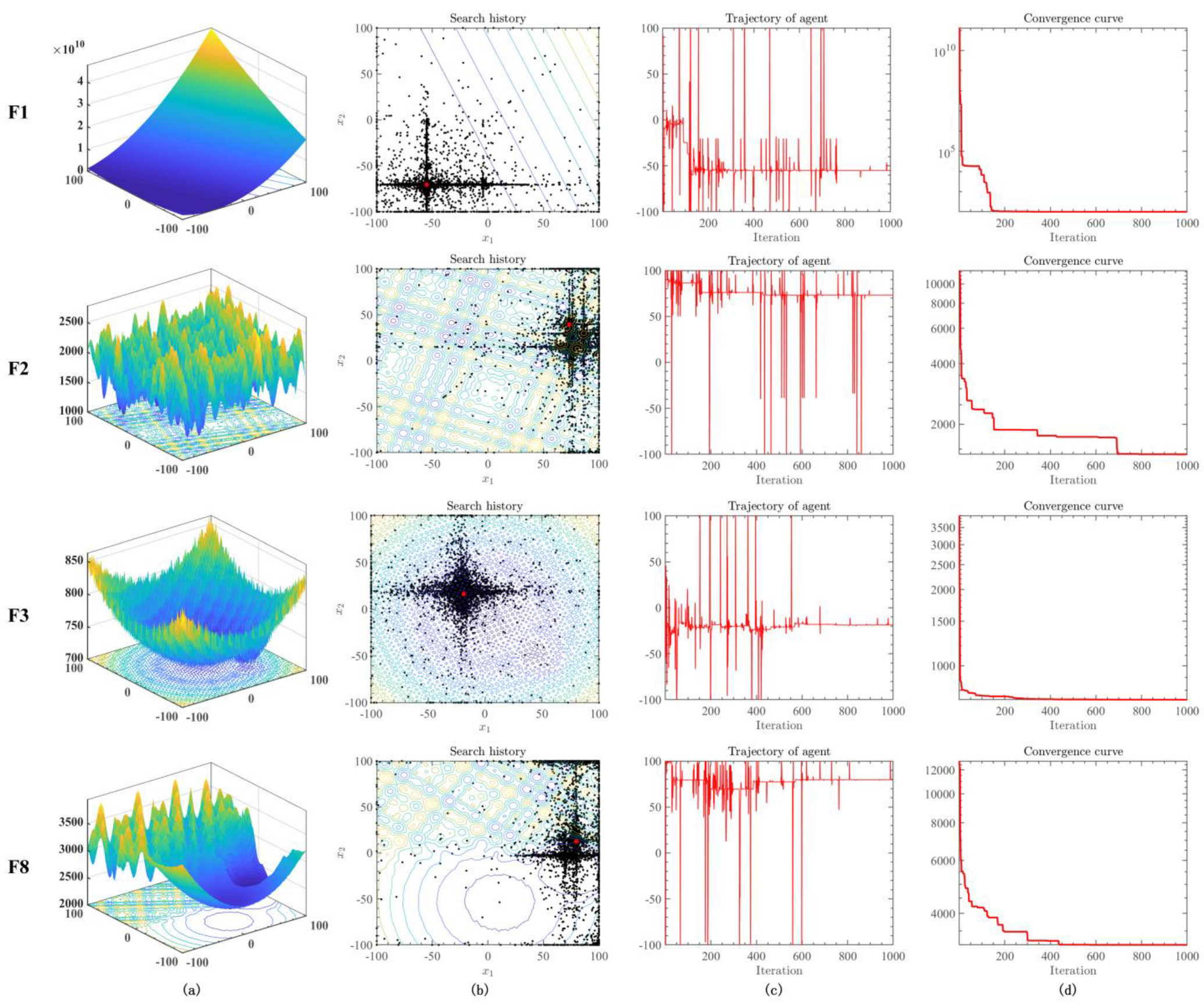
5.1. Qualitative Analysis
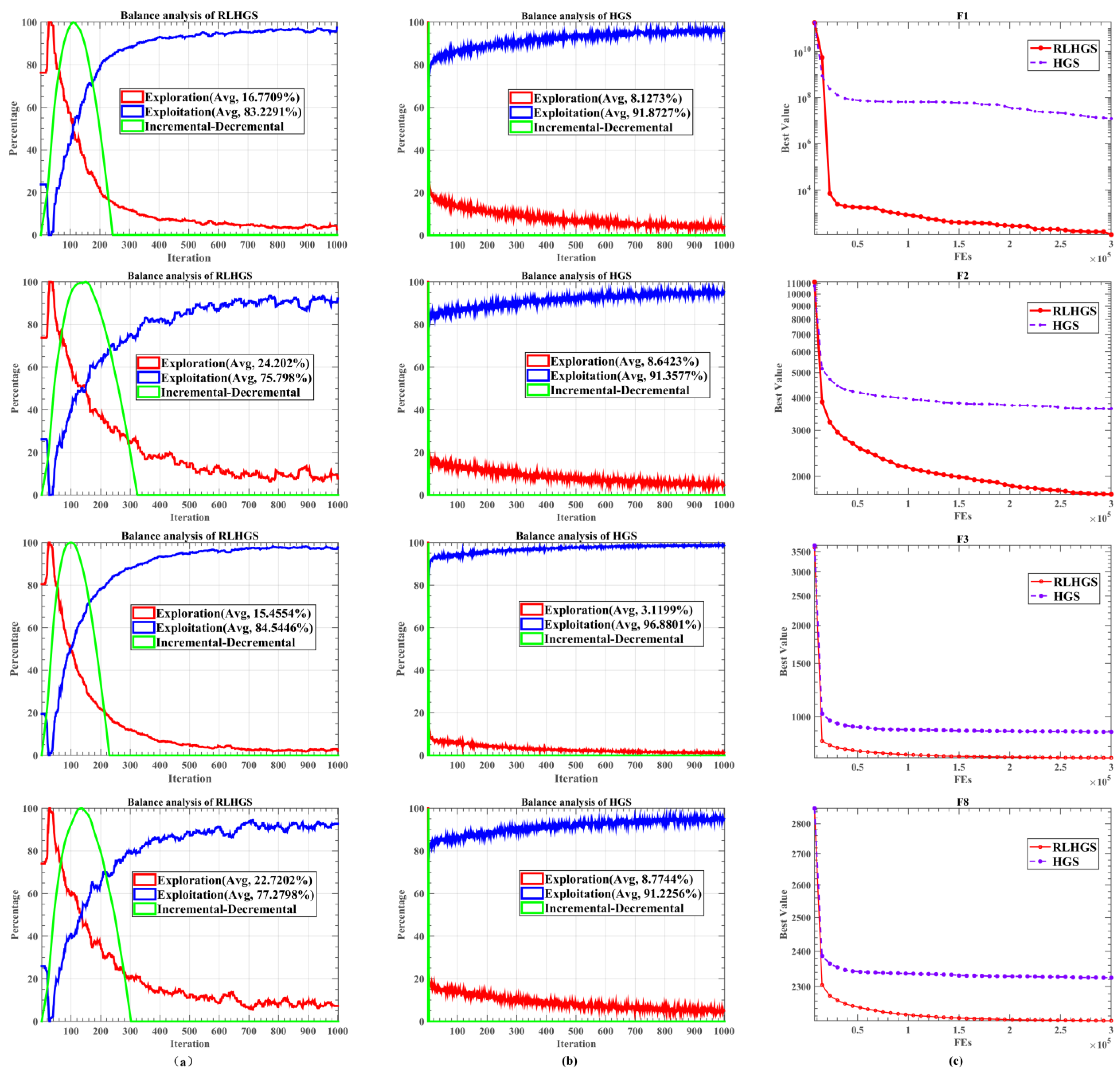
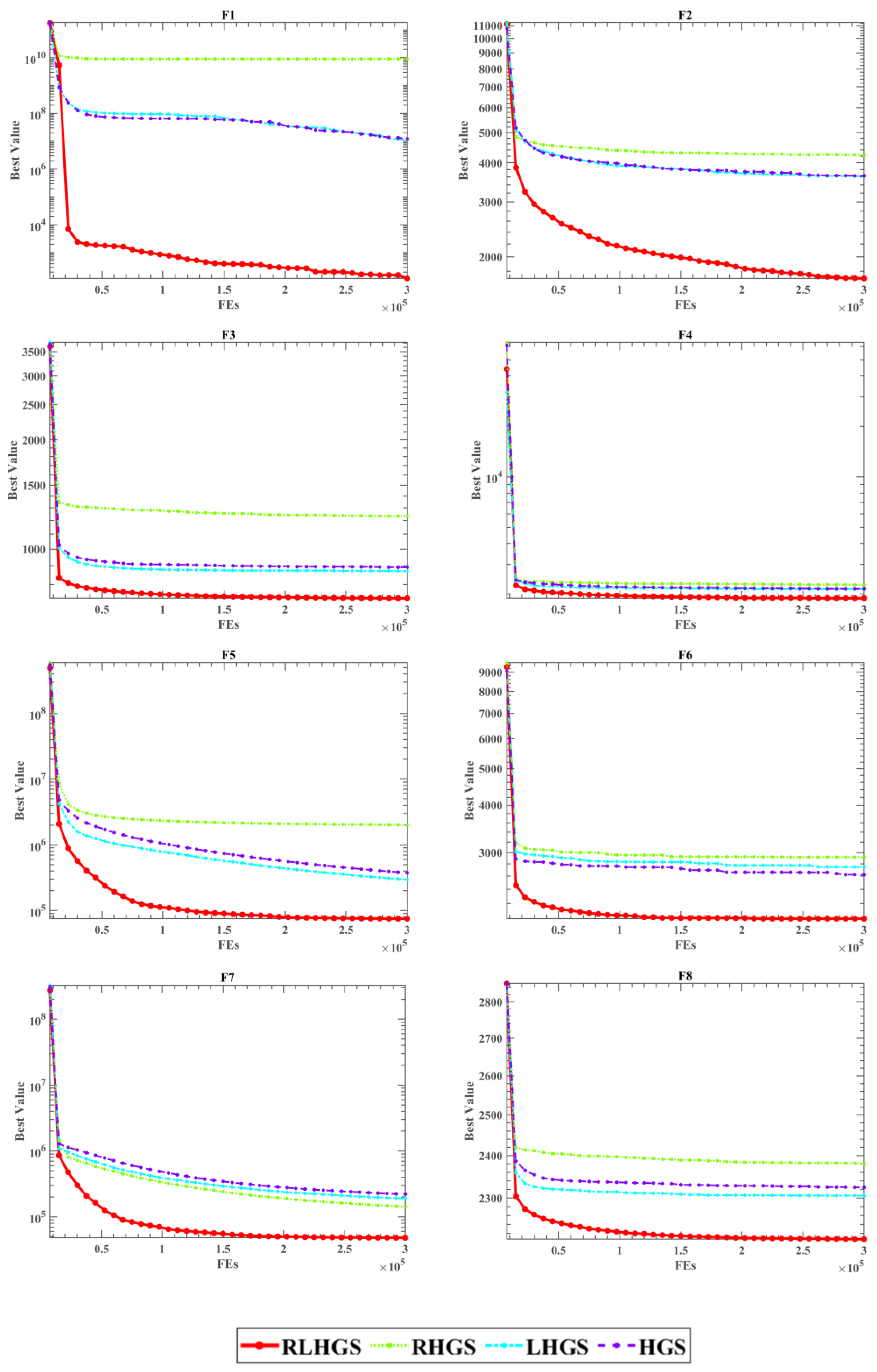
5.2. Inspection of Improvement Effect
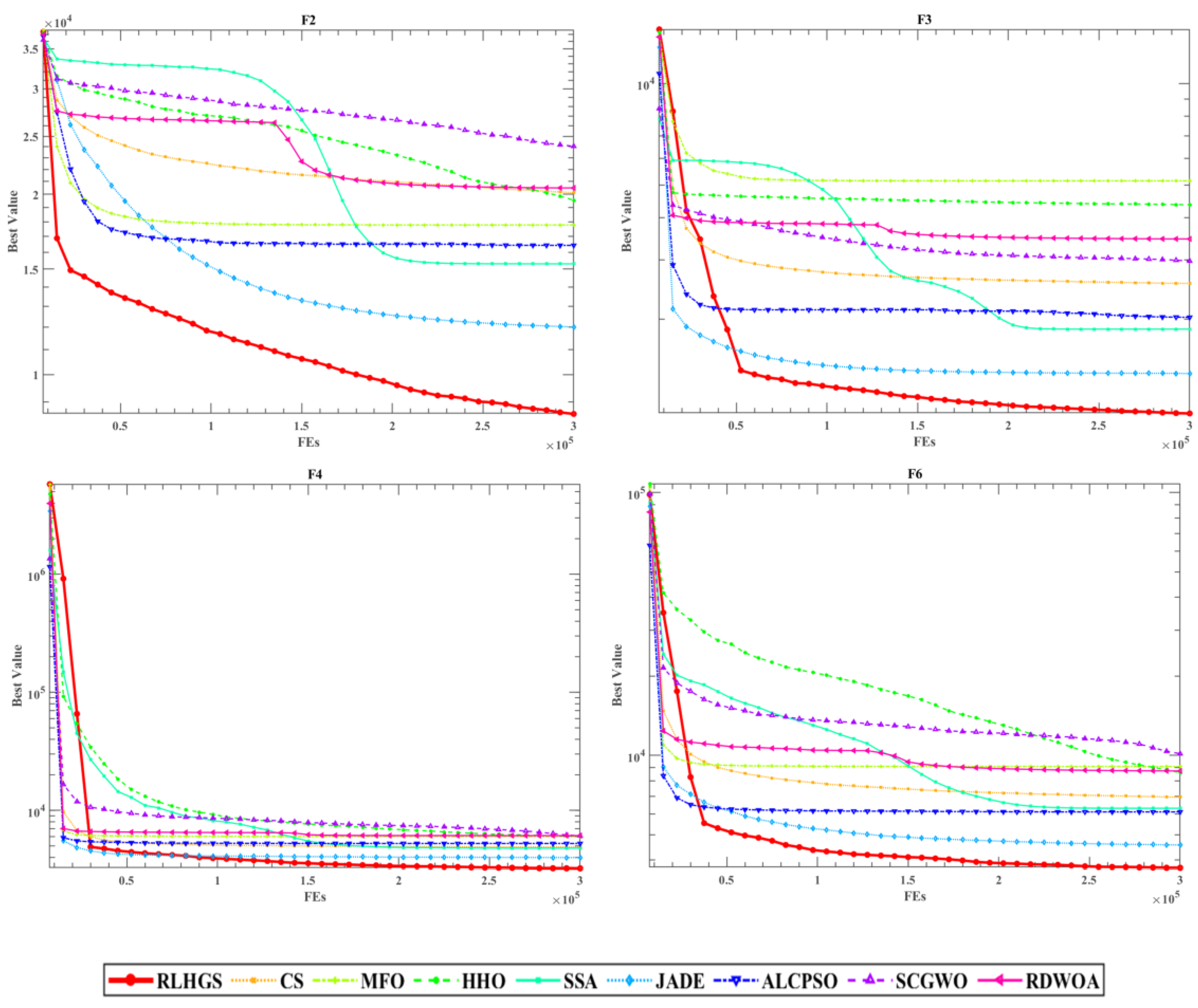
5.3. Comparison with Eight Superior Algorithms
- CS [92]: Cuckoo search algorithm, a powerful algorithm that was presented by Gandomi et al. in 2013, the internal logic of the algorithm is based on the brood parasitism of cuckoo species.
- MFO [93]: Moth-flame optimization algorithm was a novel nature-inspired heuristic paradigm proposed by Mirjalili in 2015. The inspiration for designing this algorithm origins from the navigation method of moths in nature called transverse orientation.
- HHO [27]: Harris Hawks optimization algorithm was first proposed by Heidari et al. in 2019, simulating Harris hawks’ hunting behavior.
- SSA [94]: Salp Swarm Algorithm is a bio-inspired optimization algorithm that was developed by Mirjalili et al. in 2017. The idea is based on the swarming mechanism of salps.
- JADE [95]: An adaptive differential evolution algorithm, designed by Zhang et al. in 2009, implemented with a new mutation strategy IdquoDE/current-to-best duo with optional external archive and adaptively updating control parameters into normal differential evolution algorithm.
- ALCPSO [96]: An enhanced version of particle swarm optimization raised by Chen et al. in 2013, combined with an aging leader and challenger mechanism.
- SCGWO [97]: A variant of the grey wolf optimization algorithm innovated by Hu et al. in 2021, introduced the improved spread and chaotic local search strategies to the standard grey wolf optimization.
- RDWOA [98]: An improved meta-heuristic algorithm based on the original whale optimization algorithm developed in 2019, which is equipped with a random spare strategy and double adaptive weight.
5.3.1. Benchmark Function Set I: 23 Classic Test Functions
5.3.2. Benchmark Function Set II: CEC2020 Test Functions
5.4. Four Real-World Constrained Benchmark Problems
5.4.1. Tension/Compression String Problem
5.4.2. Welded Beam Design Problem
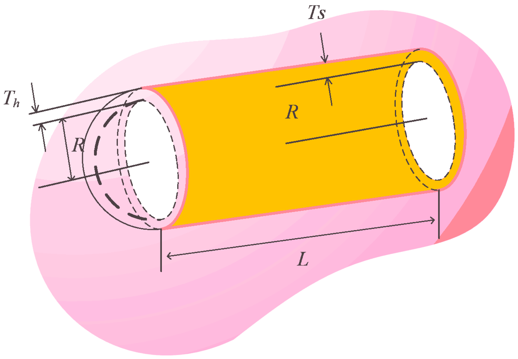
5.4.3. Pressure Vessel Design Problem
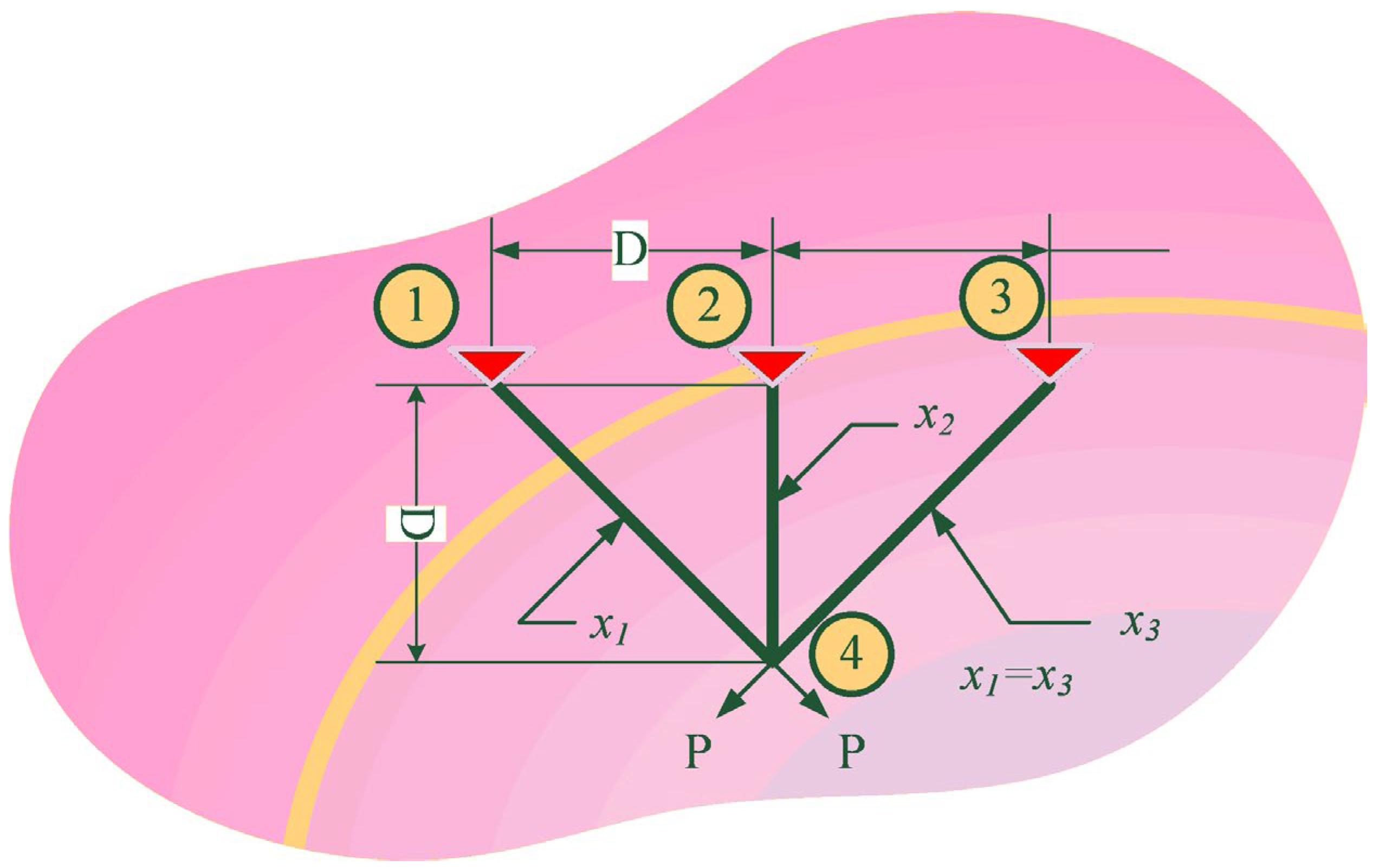
5.4.4. Three-Bar Truss Design Problem
6. Conclusions and Future Work
Author Contributions
Funding
Institutional Review Board Statement
Data Availability Statement
Acknowledgments
Conflicts of Interest
References
- Lu, Z.; Cheng, R.; Jin, Y.; Tan, K.C.; Deb, K. Neural Architecture Search as Multiobjective Optimization Benchmarks: Problem Formulation and Performance Assessment. IEEE Trans. Evol. Comput. 2022, 1. [Google Scholar] [CrossRef]
- Wang, Z.; Zhao, D.; Guan, Y. Flexible-constrained time-variant hybrid reliability-based design optimization. Struct. Multidiscip. Optim. 2023, 66, 89. [Google Scholar] [CrossRef]
- Bai, X.; Huang, M.; Xu, M.; Liu, J. Reconfiguration Optimization of Relative Motion Between Elliptical Orbits Using Lyapunov-Floquet Transformation. IEEE Trans. Aerosp. Electron. Syst. 2022, 59, 923–936. [Google Scholar] [CrossRef]
- Lu, C.; Zheng, J.; Yin, L.; Wang, R. An improved iterated greedy algorithm for the distributed hybrid flowshop scheduling problem. Eng. Optim. 2023, 1–19. [Google Scholar] [CrossRef]
- Zhang, K.; Wang, Z.; Chen, G.; Zhang, L.; Yang, Y.; Yao, C.; Wang, J.; Yao, J. Training effective deep reinforcement learning agents for real-time life-cycle production optimization. J. Pet. Sci. Eng. 2022, 208, 109766. [Google Scholar] [CrossRef]
- Li, B.; Tan, Y.; Wu, A.-G.; Duan, G.-R. A distributionally robust optimization based method for stochastic model predictive control. IEEE Trans. Autom. Control 2021, 67, 5762–5776. [Google Scholar] [CrossRef]
- Cao, B.; Zhao, J.; Yang, P.; Gu, Y.; Muhammad, K.; Rodrigues, J.J.P.C.; de Albuquerque, V.H.C. Multiobjective 3-D Topology Optimization of Next-Generation Wireless Data Center Network. IEEE Trans. Ind. Inform. 2019, 16, 3597–3605. [Google Scholar] [CrossRef]
- Cao, B.; Zhao, J.; Gu, Y.; Ling, Y.; Ma, X. Applying graph-based differential grouping for multiobjective large-scale optimization. Swarm Evol. Comput. 2020, 53, 100626. [Google Scholar] [CrossRef]
- Lv, Z.; Wu, J.; Li, Y.; Song, H. Cross-layer optimization for industrial Internet of Things in real scene digital twins. IEEE Internet Things J. 2022, 9, 15618–15629. [Google Scholar] [CrossRef]
- Selvakumar, A.I.; Thanushkodi, K. A new particle swarm optimization solution to nonconvex economic dispatch problems. IEEE Trans. Power Syst. 2007, 22, 42–51. [Google Scholar] [CrossRef]
- Li, H.Z.; Guo, S.; Li, C.J.; Sun, J.Q. A hybrid annual power load forecasting model based on generalized regression neural network with fruit fly optimization algorithm. Knowl.-Based Syst. 2013, 37, 378–387. [Google Scholar] [CrossRef]
- Kashef, S.; Nezamabadi-pour, H. An advanced ACO algorithm for feature subset selection. Neurocomputing 2015, 147, 271–279. [Google Scholar] [CrossRef]
- Mafarja, M.; Aljarah, I.; Heidari, A.A.; Faris, H.; Fournier-Viger, P.; Li, X.; Mirjalili, S. Binary dragonfly optimization for feature selection using time-varying transfer functions. Knowl.-Based Syst. 2018, 161, 185–204. [Google Scholar] [CrossRef]
- Li, J.D.; Liu, H. Challenges of Feature Selection for Big Data Analytics. Ieee Intell. Syst. 2017, 32, 9–15. [Google Scholar] [CrossRef]
- Li, Q.; Chen, H.; Huang, H.; Zhao, X.; Cai, Z.; Tong, C.; Liu, W.; Tian, X. An Enhanced Grey Wolf Optimization Based Feature Selection Wrapped Kernel Extreme Learning Machine for Medical Diagnosis. Comput. Math. Methods Med. 2017, 2017, 9512741. [Google Scholar] [CrossRef] [PubMed]
- Cao, B.; Li, M.; Liu, X.; Zhao, J.; Cao, W.; Lv, Z. Many-Objective Deployment Optimization for a Drone-Assisted Camera Network. IEEE Trans. Netw. Sci. Eng. 2021, 8, 2756–2764. [Google Scholar] [CrossRef]
- Cao, B.; Zhao, J.; Lv, Z.; Yang, P. Diversified personalized recommendation optimization based on mobile data. IEEE Trans. Intell. Transp. Syst. 2020, 22, 2133–2139. [Google Scholar] [CrossRef]
- Cao, B.; Fan, S.; Zhao, J.; Tian, S.; Zheng, Z.; Yan, Y.; Yang, P. Large-scale many-objective deployment optimization of edge servers. IEEE Trans. Intell. Transp. Syst. 2021, 22, 3841–3849. [Google Scholar] [CrossRef]
- Zhang, J.; Tang, Y.; Wang, H.; Xu, K. ASRO-DIO: Active subspace random optimization based depth inertial odometry. IEEE Trans. Robot. 2022, 39, 1496–1508. [Google Scholar] [CrossRef]
- Duan, Y.; Zhao, Y.; Hu, J. An initialization-free distributed algorithm for dynamic economic dispatch problems in microgrid: Modeling, optimization and analysis. Sustain. Energy Grids Netw. 2023, 34, 101004. [Google Scholar] [CrossRef]
- Li, R.; Wu, X.; Tian, H.; Yu, N.; Wang, C. Hybrid Memetic Pretrained Factor Analysis-Based Deep Belief Networks for Transient Electromagnetic Inversion. IEEE Trans. Geosci. Remote Sens. 2022, 60, 1–20. [Google Scholar] [CrossRef]
- Holland, J. Adaptation in Natural and Artificial Systems: An Introductory Analysis with Application to Biology; University of Michigan Press: Ann Arbor, MI, USA, 1975. [Google Scholar]
- Storn, R.; Price, K. Differential Evolution: A Simple and Efficient Adaptive Scheme for Global Optimization Over Continuous Spaces. J. Glob. Optim. 1995, 23, 341–359. [Google Scholar]
- Dan, S. Biogeography-Based Optimization. IEEE Trans. Evol. Comput. 2009, 12, 702–713. [Google Scholar]
- Kennedy, J.; Eberhart, R. Particle swarm optimization. In Proceedings of the ICNN’95-International Conference on Neural Networks, Perth, WA, Australia, 27 November–1 December 1995; Volume 4, pp. 1942–1948. [Google Scholar]
- Sm, A.; Smm, B.; Al, A. Grey Wolf Optimizer. Adv. Eng. Softw. 2014, 69, 46–61. [Google Scholar]
- Heidari, A.A.; Mirjalili, S.; Faris, H.; Aljarah, I.; Mafarja, M.; Chen, H.L. Harris hawks optimization: Algorithm and applications. Future Gener. Comput. Syst.-Int. J. Escience 2019, 97, 849–872. [Google Scholar] [CrossRef]
- Li, S.; Chen, H.; Wang, M.; Heidari, A.A.; Mirjalili, S. Slime mould algorithm: A new method for stochastic optimization. Future Gener. Comput. Syst.-Int. J. Escience 2020, 111, 300–323. [Google Scholar] [CrossRef]
- Rao, R.V.; Savsani, V.J.; Vakharia, D.P. Teaching-Learning-Based Optimization: An optimization method for continuous non-linear large scale problems. Inf. Sci. 2012, 183, 1–15. [Google Scholar] [CrossRef]
- Ramezani, F.; Lotfi, S. Social-Based Algorithm (SBA). Appl. Soft Comput. 2013, 13, 2837–2856. [Google Scholar] [CrossRef]
- Atashpaz-Gargari, E.; Lucas, C. Imperialist competitive algorithm: An algorithm for optimization inspired by imperialistic competition. In Proceedings of the 2007 IEEE Congress on Evolutionary Computation, Singapore, 25–28 September 2007; pp. 4661–4667. [Google Scholar] [CrossRef]
- Kirkpatrick, S.; Gelatt, C.D.; Vecchi, M.P. Optimization by Simulated Annealing. Science 1983, 220, 671–680. [Google Scholar] [CrossRef]
- Rashedi, E.; Nezamabadi-Pour, H.; Saryazdi, S. GSA: A Gravitational Search Algorithm. Inf. Sci. 2009, 179, 2232–2248. [Google Scholar] [CrossRef]
- Mirjalili, S.; Mirjalili, S.M.; Hatamlou, A. Multi-Verse Optimizer: A nature-inspired algorithm for global optimization. Neural Comput. Appl. 2015, 27, 495–513. [Google Scholar] [CrossRef]
- Ahmadianfar, I.; Heidari, A.A.; Gandomi, A.H.; Chu, X.; Chen, H. RUN beyond the metaphor: An efficient optimization algorithm based on Runge Kutta method. Expert Syst. Appl. 2021, 181, 115079. [Google Scholar] [CrossRef]
- Ahmadianfar, I.; Heidari, A.A.; Noshadian, S.; Chen, H.L.; Gandomi, A.H. INFO: An efficient optimization algorithm based on weighted mean of vectors. Expert Syst. Appl. 2022, 195, 116516. [Google Scholar] [CrossRef]
- Cao, B.; Gu, Y.; Lv, Z.; Yang, S.; Zhao, J.; Li, Y. RFID reader anticollision based on distributed parallel particle swarm optimization. IEEE Internet Things J. 2020, 8, 3099–3107. [Google Scholar] [CrossRef]
- Aljarah, I.; Habib, M.; Faris, H.; Al-Madi, N.; Heidari, A.A.; Mafarja, M.; Elaziz, M.A.; Mirjalili, S. A dynamic locality multi-objective salp swarm algorithm for feature selection. Comput. Ind. Eng. 2020, 147, 106628. [Google Scholar] [CrossRef]
- Houssein, E.H.; Mahdy, M.A.; Shebl, D.; Manzoor, A.; Sarkar, R.; Mohamed, W.M. An efficient slime mould algorithm for solving multi-objective optimization problems. Expert Syst. Appl. 2022, 187, 115870. [Google Scholar] [CrossRef]
- Khunkitti, S.; Siritaratiwat, A.; Premrudeepreechacharn, S. Multi-Objective Optimal Power Flow Problems Based on Slime Mould Algorithm. Sustainability 2021, 13, 7448. [Google Scholar] [CrossRef]
- Huang, F.Z.; Wang, L.; He, Q. An effective co-evolutionary differential evolution for constrained optimization. Appl. Math. Comput. 2007, 186, 340–356. [Google Scholar] [CrossRef]
- Zhang, H.; Liu, T.; Ye, X.; Heidari, A.A.; Liang, G.; Chen, H.; Pan, Z. Differential evolution-assisted salp swarm algorithm with chaotic structure for real-world problems. Eng. Comput. 2023, 39, 1735–1769. [Google Scholar] [CrossRef]
- Ji, Y.; Tu, J.; Zhou, H.; Gui, W.; Liang, G.; Chen, H.; Wang, M. An Adaptive Chaotic Sine Cosine Algorithm for Constrained and Unconstrained Optimization. Complexity 2020, 2020, 6084917. [Google Scholar] [CrossRef]
- Yang, X.; Wang, R.; Zhao, D.; Yu, F.; Huang, C.; Heidari, A.A.; Cai, Z.; Bourouis, S.; Algarni, A.D.; Chen, H. An Adaptive Quadratic Interpolation and Rounding Mechanism Sine Cosine Algorithm with Application to Constrained Engineering Optimization Problems. Expert Syst. Appl. 2020, 213, 119041. [Google Scholar] [CrossRef]
- Liu, L.; Zhao, D.; Yu, F.; Heidari, A.A.; Li, C.; Ouyang, J.; Chen, H.; Mafarja, M.; Turabieh, H.; Pan, J. Ant colony optimization with Cauchy and greedy Levy mutations for multilevel COVID 19 X-ray image segmentation. Comput. Biol. Med. 2021, 136, 104609. [Google Scholar] [CrossRef] [PubMed]
- Zhao, D.; Liu, L.; Yu, F.; Heidari, A.A.; Wang, M.; Oliva, D.; Muhammad, K.; Chen, H. Ant colony optimization with horizontal and vertical crossover search: Fundamental visions for multi-threshold image segmentation. Expert Syst. Appl. 2021, 167, 114122. [Google Scholar] [CrossRef]
- Hussien, A.G.; Heidari, A.A.; Ye, X.; Liang, G.; Chen, H.; Pan, Z. Boosting whale optimization with evolution strategy and Gaussian random walks: An image segmentation method. Eng. Comput. 2023, 39, 1935–1979. [Google Scholar] [CrossRef]
- Dutta, T.; Dey, S.; Bhattacharyya, S.; Mukhopadhyay, S. Quantum fractional order Darwinian particle swarm optimization for hyperspectral multi-level image thresholding. Appl. Soft Comput. 2021, 113, 107976. [Google Scholar] [CrossRef]
- Wang, M.; Liang, Y.; Hu, Z.; Chen, S.; Shi, B.; Heidari, A.A.; Zhang, Q.; Chen, H.; Chen, X. Lupus nephritis diagnosis using enhanced moth flame algorithm with support vector machines. Comput. Biol. Med. 2022, 145, 105435. [Google Scholar] [CrossRef] [PubMed]
- Yu, H.; Liu, J.; Chen, C.; Heidari, A.A.; Zhang, Q.; Chen, H.; Mafarja, M.; Turabieh, H. Corn Leaf Diseases Diagnosis Based on K-Means Clustering and Deep Learning. IEEE Access 2021, 9, 143824–143835. [Google Scholar] [CrossRef]
- Xia, J.; Zhang, H.; Li, R.; Chen, H.; Turabieh, H.; Mafarja, M.; Pan, Z. Generalized Oppositional Moth Flame Optimization with Crossover Strategy: An Approach for Medical Diagnosis. J. Bionic Eng. 2021, 18, 991–1010. [Google Scholar] [CrossRef]
- Liu, J.; Wei, J.; Heidari, A.A.; Kuang, F.; Zhang, S.; Gui, W.; Chen, H.; Pan, Z. Chaotic simulated annealing multi-verse optimization enhanced kernel extreme learning machine for medical diagnosis. Comput. Biol. Med. 2022, 144, 105356. [Google Scholar] [CrossRef]
- Xia, J.; Zhang, H.; Li, R.; Wang, Z.; Cai, Z.; Gu, Z.; Chen, H.; Pan, Z. Adaptive Barebones Salp Swarm Algorithm with Quasi-oppositional Learning for Medical Diagnosis Systems: A Comprehensive Analysis. J. Bionic Eng. 2022, 19, 240–256. [Google Scholar] [CrossRef]
- Yu, S.; Heidari, A.A.; He, C.; Cai, Z.; Althobaiti, M.M.; Mansour, R.F.; Liang, G.; Chen, H. Parameter estimation of static solar photovoltaic models using Laplacian Nelder-Mead hunger games search. Solar Energy 2022, 242, 79–104. [Google Scholar] [CrossRef]
- Weng, X.; Heidari, A.A.; Liang, G.; Chen, H.; Ma, X. An evolutionary Nelder–Mead slime mould algorithm with random learning for efficient design of photovoltaic models. Energy Rep. 2021, 7, 8784–8804. [Google Scholar] [CrossRef]
- Liu, Y.; Heidari, A.A.; Ye, X.; Liang, G.; Chen, H.; He, C. Boosting slime mould algorithm for parameter identification of photovoltaic models. Energy 2021, 234, 121164. [Google Scholar] [CrossRef]
- Fan, Y.; Wang, P.; Heidari, A.A.; Zhao, X.; Turabieh, H.; Chen, H. Delayed dynamic step shuffling frog-leaping algorithm for optimal design of photovoltaic models. Energy Rep. 2021, 7, 228–246. [Google Scholar] [CrossRef]
- Liu, Y.; Chong, G.; Heidari, A.A.; Chen, H.; Liang, G.; Ye, X.; Cai, Z.; Wang, M. Horizontal and vertical crossover of Harris hawk optimizer with Nelder-Mead simplex for parameter estimation of photovoltaic models. Energy Convers. Manag. 2020, 223, 113211. [Google Scholar] [CrossRef]
- Liu, Y.X.; Yang, C.N.; Sun, Q.D. Thresholds Based Image Extraction Schemes in Big Data Environment in Intelligent Traffic Management. IEEE Trans. Intell. Transp. Syst. 2021, 22, 3952–3960. [Google Scholar] [CrossRef]
- Yang, Y.T.; Chen, H.L.; Heidari, A.A.; Gandomi, A.H. Hunger games search: Visions, conception, implementation, deep analysis, perspectives, and towards performance shifts. Expert Syst. Appl. 2021, 177, 114864. [Google Scholar] [CrossRef]
- AbuShanab, W.S.; Elaziz, M.A.; Ghandourah, E.I.; Moustafa, E.B.; Elsheikh, A.H. A new fine-tuned random vector functional link model using Hunger games search optimizer for modeling friction stir welding process of polymeric materials. J. Mater. Res. Technol.-JMR T 2021, 14, 1482–1493. [Google Scholar] [CrossRef]
- Nguyen, H.; Bui, X.N. A Novel Hunger Games Search Optimization-Based Artificial Neural Network for Predicting Ground Vibration Intensity Induced by Mine Blasting. Nat. Resour. Res. 2021, 30, 3865–3880. [Google Scholar] [CrossRef]
- Xu, B.Y.; Heidari, A.A.; Kuang, F.J.; Zhang, S.Y.; Chen, H.L.; Cai, Z.N. Quantum Nelder-Mead Hunger Games Search for optimizing photovoltaic solar cells. Int. J. Energy Res. 2022, 46, 12417–12466. [Google Scholar] [CrossRef]
- Ma, B.J.; Liu, S.; Heidari, A.A. Multi-strategy ensemble binary hunger games search for feature selection. Knowl.-Based Syst. 2022, 248, 108787. [Google Scholar] [CrossRef]
- Fathy, A.; Yousri, D.; Rezk, H.; Thanikanti, S.B.; Hasanien, H.M. A Robust Fractional-Order PID Controller Based Load Frequency Control Using Modified Hunger Games Search Optimizer. Energies 2022, 15, 361. [Google Scholar] [CrossRef]
- Emam, M.M.; Samee, N.A.; Jamjoom, M.M.; Houssein, E.H. Optimized deep learning architecture for brain tumor classification using improved Hunger Games Search Algorithm. Comput. Biol. Med. 2023, 160, 106966. [Google Scholar] [CrossRef] [PubMed]
- Nassef, A.M.; Houssein, E.H.; Rezk, H.; Fathy, A. Optimal Allocation of Biomass Distributed Generators Using Modified Hunger Games Search to Reduce CO2 Emissions. J. Mar. Sci. Eng. 2023, 11, 308. [Google Scholar] [CrossRef]
- Zhang, Y.; Guo, Y.; Xiao, Y.; Tang, W.; Zhang, H.; Li, J. A novel hybrid improved hunger games search optimizer with extreme learning machine for predicting shrinkage of SLS parts. J. Intell. Fuzzy Syst. 2022, 43, 5643–5659. [Google Scholar] [CrossRef]
- Chen, Z.; Xuan, P.; Heidari, A.A.; Liu, L.; Wu, C.; Chen, H.; Escorcia-Gutierrez, J.; Mansour, R.F. An artificial bee bare-bone hunger games search for global optimization and high-dimensional feature selection. Iscience 2023, 26, 106679. [Google Scholar] [CrossRef] [PubMed]
- Wolpert, D.H.; Macready, W.G. No free lunch theorems for optimization. IEEE Trans. Evol. Comput. 1997, 1, 67–82. [Google Scholar] [CrossRef]
- Li, C.; Li, J.; Chen, H.; Jin, M.; Ren, H. Enhanced Harris hawks optimization with multi-strategy for global optimization tasks. Expert Syst. Appl. 2021, 185, 115499. [Google Scholar] [CrossRef]
- Real, L.A. Animal Choice Behavior and the Evolution of cognitive Architecture. Science 1991, 253, 980–986. [Google Scholar] [CrossRef]
- Burnett, C.J.; Li, C.; Webber, E.; Tsaousidou, E.; Xue, S.Y.; Brüning, J.C.; Krashes, M.J. Hunger-Driven Motivational State Competition. Neuron 2016, 92, 187–201. [Google Scholar] [CrossRef]
- O’Brien, W.J.; Browman, H.I.; Evans, B.I. Search strategies of foraging animals. Am. Sci. 1990, 78, 152–160. [Google Scholar]
- Clutton-Brock, T. Cooperation between non-kin in animal societies. Nature 2009, 462, 51–57. [Google Scholar] [CrossRef] [PubMed]
- Friedman, M.I.; Ulrich, P.; Mattes, R.D. A figurative measure of subjective hunger sensations. Appetite 1999, 32, 395–404. [Google Scholar] [CrossRef] [PubMed]
- Zhou, X.; Gui, W.; Heidari, A.A.; Cai, Z.; Elmannai, H.; Hamdi, M.; Liang, G.; Chen, H. Advanced orthogonal learning and Gaussian barebone hunger games for engineering design. J. Comput. Des. Eng. 2022, 9, 1699–1736. [Google Scholar] [CrossRef]
- Tamura, K.; Yasuda, K. Primary Study of Spiral Dynamics Inspired Optimization. IEEJ Trans. Electr. Electron. Eng. 2011, 6, S98–S100. [Google Scholar] [CrossRef]
- Kawaguchi, Y. A morphological study of the form of nature. ACM Siggraph Comput. Graph. 1982, 16, 223–232. [Google Scholar] [CrossRef]
- Rahnamayan, S.; Tizhoosh, H.R.; Salama, M.M.A. Opposition-based differential evolution. IEEE Trans. Evol. Comput. 2008, 12, 64–79. [Google Scholar] [CrossRef]
- Rosenbrock, H.H. An Automatic Method for Finding the Greatest or Least Value of a Function. Comput. J. 1960, 3, 175–184. [Google Scholar] [CrossRef]
- Kang, F.; Li, J.J.; Ma, Z.Y. Rosenbrock artificial bee colony algorithm for accurate global optimization of numerical functions. Inf. Sci. 2011, 181, 3508–3531. [Google Scholar] [CrossRef]
- Xin, Y.; Yong, L.; Guangming, L. Evolutionary programming made faster. IEEE Trans. Evol. Comput. 1999, 3, 82–102. [Google Scholar] [CrossRef]
- Viktorin, A.; Senkerik, R.; Pluhacek, M.; Kadavy, T.; Zamuda, A. DISH-XX Solving CEC2020 Single Objective Bound Constrained Numerical optimization Benchmark. In Proceedings of the 2020 IEEE Congress on Evolutionary Computation (CEC), Glasgow, UK, 19–24 July 2020; pp. 1–8. [Google Scholar]
- Wang, S.; Hu, X.; Sun, J.; Liu, J. Hyperspectral anomaly detection using ensemble and robust collaborative representation. Inf. Sci. 2023, 624, 748–760. [Google Scholar] [CrossRef]
- Cheng, L.; Yin, F.; Theodoridis, S.; Chatzis, S.; Chang, T.-H. Rethinking Bayesian learning for data analysis: The art of prior and inference in sparsity-aware modeling. IEEE Signal Process. Mag. 2022, 39, 18–52. [Google Scholar] [CrossRef]
- Zhang, X.; Wen, S.; Yan, L.; Feng, J.; Xia, Y. A Hybrid-Convolution Spatial–Temporal Recurrent Network For Traffic Flow Prediction. Comput. J. 2022, bxac171. [Google Scholar] [CrossRef]
- Xu, J.; Mu, B.; Zhang, L.; Chai, R.; He, Y.; Zhang, X. Fabrication and optimization of passive flexible ammonia sensor for aquatic supply chain monitoring based on adaptive parameter adjustment artificial neural network (APA-ANN). Comput. Electron. Agric. 2023, 212, 108082. [Google Scholar] [CrossRef]
- Liu, H.; Yue, Y.; Liu, C.; Jr, B.S.; Cui, J. Automatic recognition and localization of underground pipelines in GPR B-scans using a deep learning model. Tunn. Undergr. Space Technol. 2023, 134, 104861. [Google Scholar] [CrossRef]
- Friedman, M. The Use of Ranks to Avoid the Assumption of Normality Implicit in the Analysis of Variance. J. Am. Stat. Assoc. 1937, 32, 675–701. [Google Scholar] [CrossRef]
- Garcia, S.; Fernandez, A.; Luengo, J.; Herrera, F. Advanced nonparametric tests for multiple comparisons in the design of experiments in computational intelligence and data mining: Experimental analysis of power. Inf. Sci. 2010, 180, 2044–2064. [Google Scholar] [CrossRef]
- Gandomi, A.H.; Yang, X.-S.; Alavi, A.H. Cuckoo search algorithm: A metaheuristic approach to solve structural optimization problems. Eng. Comput. 2013, 29, 17–35. [Google Scholar] [CrossRef]
- Mirjalili, S. Moth-flame optimization algorithm: A novel nature-inspired heuristic paradigm. Knowl.-Based Syst. 2015, 89, 228–249. [Google Scholar] [CrossRef]
- Mirjalili, S.; Gandomi, A.H.; Mirjalili, S.Z.; Saremi, S.; Faris, H.; Mirjalili, S.M. Salp Swarm Algorithm: A bio-inspired optimizer for engineering design problems. Adv. Eng. Softw. 2017, 114, 163–191. [Google Scholar] [CrossRef]
- Zhang, J.; Sanderson, A.C. JADE: Adaptive Differential Evolution With Optional External Archive. IEEE Trans. Evol. Comput. 2009, 13, 945–958. [Google Scholar] [CrossRef]
- Chen, W.-N.; Zhang, J.; Lin, Y.; Chen, N.; Zhan, Z.-H.; Chung, H.S.-H.; Li, Y.; Shi, Y.-H. Particle Swarm Optimization with an Aging Leader and Challengers. IEEE Trans. Evol. Comput. 2013, 17, 241–258. [Google Scholar] [CrossRef]
- Hu, J.; Heidari, A.A.; Zhang, L.; Xue, X.; Gui, W.; Chen, H.; Pan, Z. Chaotic diffusion-limited aggregation enhanced grey wolf optimizer: Insights, analysis, binarization, and feature selection. Int. J. Intell. Syst. 2021, 37, 4864–4927. [Google Scholar] [CrossRef]
- Chen, H.; Xu, Y.; Wang, M.; Zhao, X. A balanced whale optimization algorithm for constrained engineering design problems. Appl. Math. Model. 2019, 71, 45–59. [Google Scholar] [CrossRef]
- Mezura-Montes, E.; Coello, C.A.C. Constraint-handling in nature-inspired numerical optimization: Past, present and future. Swarm Evol. Comput. 2011, 1, 173–194. [Google Scholar] [CrossRef]
- Mahdavi, M.; Fesanghary, M.; Damangir, E. An improved harmony search algorithm for solving optimization problems. Appl. Math. Comput. 2007, 188, 1567–1579. [Google Scholar] [CrossRef]
- Mirjalili, S.; Lewis, A. The Whale Optimization Algorithm. Adv. Eng. Softw. 2016, 95, 51–67. [Google Scholar] [CrossRef]
- Chen, C.; Wang, X.; Yu, H.; Wang, M.; Chen, H. Dealing with multi-modality using synthesis of Moth-flame optimizer with sine cosine mechanisms. Math. Comput. Simul. 2021, 188, 291–318. [Google Scholar] [CrossRef]
- Lee, K.S.; Geem, Z.W. A new meta-heuristic algorithm for continuous engineering optimization: Harmony search theory and practice. Comput. Methods Appl. Mech. Eng. 2005, 194, 3902–3933. [Google Scholar] [CrossRef]
- Gandomi, A.H.; Yang, X.S.; Alavi, A.H.; Talatahari, S. Bat algorithm for constrained optimization tasks. Neural Comput. Appl. 2013, 22, 1239–1255. [Google Scholar] [CrossRef]
- Kaveh, A.; Khayatazad, M. A new meta-heuristic method: Ray Optimization. Comput. Struct. 2012, 112, 283–294. [Google Scholar] [CrossRef]
- Ragsdell, K.M.; Phillips, D.T. Optimal Design of a Class of Welded Structures Using Geometric Programming. J. Eng. Ind. 1976, 98, 1021–1025. [Google Scholar] [CrossRef]
- Mezura-Montes, E.; Coello, C.A.C. An empirical study about the usefulness of evolution strategies to solve constrained optimization problems. Int. J. Gen. Syst. 2008, 37, 443–473. [Google Scholar] [CrossRef]
- Coelho, L.D. Gaussian quantum-behaved particle swarm optimization approaches for constrained engineering design problems. Expert Syst. Appl. 2010, 37, 1676–1683. [Google Scholar] [CrossRef]
- Sandgren, E. Nonlinear Integer and Discrete Programming in Mechanical Design Optimization. J. Mech. Des. 1990, 112, 223–229. [Google Scholar] [CrossRef]
- He, Q.; Wang, L. An effective co-evolutionary particle swarm optimization for constrained engineering design problems. Eng. Appl. Artif. Intell. 2007, 20, 89–99. [Google Scholar] [CrossRef]
- Saremi, S.; Mirjalili, S.; Lewis, A. Grasshopper optimisation algorithm: Theory and application. Adv. Eng. Softw. 2017, 105, 30–47. [Google Scholar] [CrossRef]
- Sadollah, A.; Bahreininejad, A.; Eskandar, H.; Hamdi, M. Mine blast algorithm: A new population based algorithm for solving constrained engineering optimization problems. Appl. Soft Comput. 2013, 13, 2592–2612. [Google Scholar] [CrossRef]


| Type | MAs | Published | Brief Introduction |
|---|---|---|---|
| Evolutionary-based | Genetic Algorithm (GA) [22] | 1975 | It is derived from biological, genetic, and evolutionary mechanisms and an adaptive probabilistic optimization algorithm. |
| Differential Evolution (DE) [23] | 1995 | It can be considered based on the theory of biological evolution, which imitates the process of cooperation and competition among individuals. | |
| Biogeography-Based Optimization (BBO) [24] | 2008 | It is based on the geographical distribution of biological organisms. | |
| Swarm intelligence-based | Particle Swarm Optimization (PSO) [25] | 1995 | It is inspired by the collective behavior of social organisms, particularly the flocking and swarming behavior observed in birds, fish, and insects. |
| Grey Wolf Optimization (GWO) [26] | 2014 | Its inspiration is from observing the leadership level and hunting behaviors within grey wolves in nature. | |
| Harris Hawk Optimization (HHO) [27] | 2019 | It draws upon the natural behavior of wolf pack hunting. | |
| Slime Mould Algorithm (SMA) [28] | 2020 | Its principle is based on the oscillation mode of slime moulds in nature. | |
| Human behavior-based | Teaching-Learning-Based Optimization (TLBO) [29] | 2011 | It is inspired by the idea of how teachers guide students toward better learning outcomes. |
| Social-Based Algorithm (SBA) [30] | 2013 | It is in the light of the evolutionary algorithm and socio-political process based Imperialist Competitive Algorithm (ICA) [31]. | |
| Physics-based | Simulated Annealing (SA) [32] | 1983 | It is proposed based on the principle of solid-state high-temperature annealing. |
| Gravitational Search Algorithm (GSA) [33] | 2009 | It can trace back to the law of gravity and mass interactions. | |
| Multi-Verse Optimizer (MVO) [34] | 2015 | It is according to three cosmology concepts: white hole, black hole, and wormhole. | |
| RUNge Kutta Optimizer (RUN) [35] | 2021 | It combines elements of the classical Runge-Kutta numerical integration method with optimization techniques. | |
| weIghted meaN oF vectOrs (INFO) [36] | 2022 | It stems from the weight mean method, which is an enhanced optimizer in solving optimization problems. |
| Function | |||
|---|---|---|---|
| 30 | [−100, 100] | 0 | |
| 30 | [−10, 10] | 0 | |
| 30 | [−100, 100] | 0 | |
| 30 | [−100, 100] | 0 | |
| 30 | [−30, 30] | 0 | |
| 30 | [−100, 100] | 0 | |
| 30 | [−1.28, 1.28] | 0 | |
| 30 | [−500, 500] | −418.9829 × 30 | |
| 30 | [−5.12, 5.12] | 0 | |
| 30 | [−32, 32] | 0 | |
| 30 | [−600, 600] | 0 | |
| 30 | [−50, 50] | 0 | |
| 30 | [−50, 50] | 0 | |
| 2 | [−65, 65] | 1 | |
| 4 | [−5, 5] | 0.00030 | |
| 2 | [−5, 5] | −1.0316 | |
| 2 | [−5, 5] | 0.398 | |
| 2 | [−2, 2] | 3 | |
| 3 | [1, 3] | −3.86 | |
| 6 | [0, 1] | −3.32 | |
| 4 | [0, 10] | −10.1532 | |
| 4 | [0, 10] | −10.4028 | |
| 4 | [0, 10] | −10.5363 |
| No. | Function | |
|---|---|---|
| Shifted and Rotated Bent Cigar Function | 100 | |
| Shifted and Rotated Schwefel’s Function | 1100 | |
| Shifted and Rotated Lunacek bi-Rastrigin Function | 700 | |
| Expanded Rosenbrock’s plus Criewangk’s Function | 1900 | |
| Hybrid Function 1 (N = 3) | 1700 | |
| Hybrid Function 2 (N = 4) | 1600 | |
| Hybrid Function 3 (N = 5) | 2100 | |
| Composition Function 1 (N = 3) | 2200 | |
| Composition Function 2 (N = 4) | 2400 | |
| Composition Function 3 (N = 5) | 2500 |
| Algorithm | LS-OBL Strategy | Adapted RM Strategy |
|---|---|---|
| RLHGS | 1 | 1 |
| RHGS | 0 | 1 |
| LHGS | 1 | 0 |
| HGS | 0 | 0 |
| F1 | F2 | F3 | |||||||
| Avg | Std | Rank | Avg | Std | Rank | Avg | Std | Rank | |
| RLHGS | 1.1721 × 10² | 3.8415 × 101 | 1 | 1.7057 × 10³ | 2.1073 × 10² | 1 | 7.3244 × 10² | 1.0536 × 101 | 1 |
| RHGS | 9.1127 × 10⁹ | 1.3465 × 10¹⁰ | 4 | 4.2311 × 10³ | 6.1760 × 10² | 4 | 1.2333 × 10³ | 1.6875 × 10² | 4 |
| LHGS | 1.1411 × 10⁷ | 2.5083 × 10⁷ | 2 | 3.6214 × 10³ | 5.0565 × 10² | 2 | 8.7070 × 10² | 5.5928 × 101 | 2 |
| HGS | 1.2428 × 10⁷ | 3.4529 × 10⁷ | 3 | 3.6354 × 10³ | 4.8399 × 10² | 3 | 8.9153 × 10² | 4.6783 × 101 | 3 |
| F4 | F5 | F6 | |||||||
| Avg | Std | Rank | Avg | Std | Rank | Avg | Std | Rank | |
| RLHGS | 1.8836 × 10³ | 8.9986 × 101 | 1 | 7.4880 × 10⁴ | 4.3342 × 10⁴ | 1 | 2.0053 × 10³ | 1.5192 × 10² | 1 |
| RHGS | 2.2603 × 10³ | 1.5553 × 10² | 4 | 2.0131 × 10⁶ | 7.3692 × 10⁶ | 4 | 2.9175 × 10³ | 3.4464 × 10² | 4 |
| LHGS | 2.1305 × 10³ | 1.9996 × 10² | 2 | 2.9555 × 10⁵ | 2.0583 × 10⁵ | 2 | 2.7490 × 10³ | 2.8624 × 10² | 3 |
| HGS | 2.1426 × 10³ | 1.5782 × 10² | 3 | 3.7466 × 10⁵ | 2.8119 × 10⁵ | 3 | 2.6231 × 10³ | 2.8102 × 10² | 2 |
| F7 | F8 | F9 | |||||||
| Avg | Std | Rank | Avg | Std | Rank | Avg | Std | Rank | |
| RLHGS | 4.8111 × 10⁴ | 3.1322 × 10⁴ | 1 | 2.2069 × 10³ | 2.2097 × 100 | 1 | 3.1351 × 10³ | 3.5632 × 10² | 3 |
| RHGS | 1.4287 × 10⁵ | 1.2640 × 10⁵ | 2 | 2.3809 × 10³ | 2.9696 × 101 | 4 | 2.6000 × 10³ | 7.2642 × 10⁻¹³ | 1 |
| LHGS | 1.8992 × 10⁵ | 1.3637 × 10⁵ | 3 | 2.3053 × 10³ | 3.2974 × 101 | 2 | 3.1590 × 10³ | 4.0319 × 10² | 4 |
| HGS | 2.2062 × 10⁵ | 1.7583 × 10⁵ | 4 | 2.3246 × 10³ | 3.3913 × 101 | 3 | 2.6000 × 10³ | 0.0000 × 100 | 1 |
| F10 | |||||||||
| Avg | Std | Rank | +/−/= | ||||||
| RLHGS | 2.8647 × 10³ | 7.4926 × 101 | 4 | ~ | |||||
| RHGS | 2.7000 × 10³ | 4.3058 × 10⁻¹³ | 1 | 8/2/0 | |||||
| LHGS | 2.7797 × 10³ | 1.3715 × 10² | 3 | 8/1/1 | |||||
| HGS | 2.7000 × 10³ | 0.0000 × 100 | 1 | 8/2/0 |
| RLHGS | RHGS | LHGS | HGS | |
|---|---|---|---|---|
| Average rank | 1.5 | 3.2 | 2.5 | 2.6 |
| Overall rank | 1 | 4 | 2 | 3 |
| RHGS | LHGS | HGS | |
|---|---|---|---|
| F1 | 1.7344 × 10⁻⁶ | 1.7344 × 10⁻⁶ | 1.7344 × 10⁻⁶ |
| F2 | 1.7344 × 10⁻⁶ | 1.7344 × 10⁻⁶ | 1.7344 × 10⁻⁶ |
| F3 | 1.7344 × 10⁻⁶ | 1.7344 × 10⁻⁶ | 1.7344 × 10⁻⁶ |
| F4 | 2.3534 × 10⁻⁶ | 3.7243 × 10⁻⁵ | 5.2165 × 10⁻⁶ |
| F5 | 1.6046 × 10⁻⁴ | 1.9729 × 10⁻⁵ | 2.3534 × 10⁻⁶ |
| F6 | 1.9209 × 10⁻⁶ | 1.7344 × 10⁻⁶ | 3.5152 × 10⁻⁶ |
| F7 | 3.3173 × 10⁻⁴ | 9.3157 × 10⁻⁶ | 7.6909 × 10⁻⁶ |
| F8 | 1.7344 × 10⁻⁶ | 1.7344 × 10⁻⁶ | 1.7344 × 10⁻⁶ |
| F9 | 4.6072 × 10⁻⁵ | 1.5140 × 10⁻¹ | 5.9493 × 10⁻⁵ |
| F10 | 1.2290 × 10⁻⁵ | 2.0297 × 10⁻³ | 1.2290 × 10⁻⁵ |
| Algorithm | Parameter | Value |
|---|---|---|
| RLHGS | 0.03 | |
| 100 | ||
| 50 | ||
| −0.5 | ||
| HGS | 0.03 | |
| 100 | ||
| CS | 0 | |
| 0.25 | ||
| MFO | 1 | |
| [−2, 1] | ||
| HHO | 1.5 | |
| SSA | [0, 1] | |
| [0, 1] | ||
| JADE | 0.1 | |
| 0.05 | ||
| 0.5 | ||
| 0.5 | ||
| ALCPSO | 0.4 | |
| 2 | ||
| 2 | ||
| 60 | ||
| 2 | ||
| SCGWO | [2, 0] | |
| 2 | ||
| RDWOA | [2, 0] | |
| [−2, −1] | ||
| 1 | ||
| 0 |
| F1 | F2 | F3 | |||||||
| Avg | Std | Rank | Avg | Std | Rank | Avg | Std | Rank | |
| RLHGS | 0.0000 × 100 | 0.0000 × 100 | 1 | 0.0000 × 100 | 0.0000 × 100 | 1 | 4.8140 × 10⁻¹ | 2.6367 × 100 | 4 |
| CS | 1.0136 × 10⁻⁶ | 7.1003 × 10⁻⁷ | 8 | 1.0000 × 10¹⁰ | 0.0000 × 100 | 9 | 2.7749 × 10³ | 3.6176 × 10² | 7 |
| MFO | 1.9684 × 10⁴ | 1.1885 × 10⁴ | 9 | 1.4177 × 10² | 3.8959 × 101 | 8 | 1.2467 × 10⁵ | 7.6037 × 10⁴ | 9 |
| HHO | 0.0000 × 100 | 0.0000 × 100 | 1 | 0.0000 × 100 | 0.0000 × 100 | 1 | 0.0000 × 100 | 0.0000 × 100 | 1 |
| SSA | 7.0715 × 10⁻⁸ | 6.9886 × 10⁻⁹ | 7 | 6.0408 × 100 | 2.7973 × 100 | 7 | 1.8429 × 10³ | 5.7033 × 10² | 6 |
| JADE | 3.7971 × 10−54 | 2.0335 × 10−53 | 5 | 7.8126 × 10⁻²¹ | 4.2783 × 10⁻²⁰ | 5 | 5.1594 × 10⁻¹ | 1.7506 × 100 | 7 |
| ALCPSO | 5.5275 × 10⁻⁸ | 3.0275 × 10⁻⁷ | 6 | 2.8912 × 10⁻¹ | 3.9540 × 10⁻¹ | 6 | 4.3973 × 10⁴ | 4.9839 × 10⁴ | 8 |
| SCGWO | 0.0000 × 100 | 0.0000 × 100 | 1 | 1.6093 × 10−306 | 0.0000 × 100 | 4 | 0.0000 × 100 | 0.0000 × 100 | 1 |
| RDWOA | 0.0000 × 100 | 0.0000 × 100 | 1 | 0.0000 × 100 | 0.0000 × 100 | 1 | 0.0000 × 100 | 0.0000 × 100 | 1 |
| F4 | F5 | F6 | |||||||
| Avg | Std | Rank | Avg | Std | Rank | Avg | Std | Rank | |
| RLHGS | 1.3092 × 100 | 3.6868 × 100 | 4 | 4.9487 × 101 | 3.4040 × 101 | 3 | 4.6288 × 10⁻¹¹ | 1.3740 × 10⁻¹⁰ | 2 |
| CS | 2.1938 × 101 | 2.6548 × 100 | 5 | 2.8015 × 10² | 8.1279 × 101 | 8 | 9.4781 × 10⁻⁷ | 7.5517 × 10⁻⁷ | 4 |
| MFO | 9.3119 × 101 | 2.7711 × 100 | 9 | 3.2477 × 10⁷ | 4.4852 × 10⁷ | 9 | 2.2485 × 10⁴ | 1.4372 × 10⁴ | 9 |
| HHO | 0.0000 × 100 | 0.0000 × 100 | 1 | 2.9834 × 10⁻⁴ | 4.0764 × 10⁻⁴ | 2 | 2.4328 × 10⁻⁶ | 3.4989 × 10⁻⁶ | 5 |
| SSA | 2.3199 × 101 | 3.5560 × 100 | 6 | 1.5513 × 10² | 1.0766 × 10² | 6 | 6.9376 × 10⁻⁸ | 6.2853 × 10⁻⁹ | 3 |
| JADE | 3.0183 × 101 | 2.5466 × 100 | 7 | 6.2184 × 101 | 4.8003 × 101 | 4 | 4.1087 × 10⁻³² | 2.7731 × 10⁻³² | 1 |
| ALCPSO | 4.6584 × 101 | 5.0435 × 100 | 8 | 1.7682 × 10² | 5.6304 × 101 | 7 | 2.5553 × 10⁻⁵ | 1.3996 × 10⁻⁴ | 8 |
| SCGWO | 0.0000 × 100 | 0.0000 × 100 | 1 | 6.7320 × 10⁻⁵ | 2.1095 × 10⁻⁴ | 1 | 4.6217 × 10⁻⁶ | 6.9114 × 10⁻⁶ | 6 |
| RDWOA | 0.0000 × 100 | 0.0000 × 100 | 1 | 9.0644 × 101 | 4.7346 × 10⁻¹ | 5 | 2.1185 × 10⁻⁵ | 1.1602 × 10⁻⁴ | 7 |
| F7 | F8 | F9 | |||||||
| Avg | Std | Rank | Avg | Std | Rank | Avg | Std | Rank | |
| RLHGS | 8.4687 × 10⁻² | 1.1647 × 10⁻¹ | 5 | −3.7931 × 10⁴ | 7.4989 × 10³ | 5 | 0.0000 × 100 | 0.0000 × 100 | 1 |
| CS | 4.2060 × 10⁻¹ | 9.4582 × 10⁻² | 7 | −2.6888 × 10⁴ | 8.2358 × 10² | 7 | 2.0495 × 10² | 3.0866 × 101 | 6 |
| MFO | 1.6836 × 10² | 1.2589 × 10² | 9 | −2.4513 × 10⁴ | 2.3311 × 10³ | 9 | 6.5040 × 10² | 9.4359 × 101 | 9 |
| HHO | 1.3552 × 10⁻⁵ | 1.2912 × 10⁻⁵ | 1 | −4.1898 × 10⁴ | 1.5437 × 10⁻² | 2 | 0.0000 × 100 | 0.0000 × 100 | 1 |
| SSA | 1.4539 × 10⁻¹ | 3.3744 × 10⁻² | 6 | −2.4613 × 10⁴ | 1.5061 × 10³ | 8 | 2.1037 × 10² | 4.3408 × 101 | 7 |
| JADE | 7.7322 × 10⁻² | 2.2043 × 10⁻² | 4 | −4.0706 × 10⁴ | 3.5996 × 10² | 4 | 1.3266 × 10⁻¹ | 3.4400 × 10⁻¹ | 5 |
| ALCPSO | 9.5572 × 10⁻¹ | 4.4139 × 10⁻¹ | 8 | −3.2131 × 10⁴ | 1.4817 × 10³ | 6 | 3.5699 × 10² | 5.1277 × 101 | 8 |
| SCGWO | 1.6531 × 10⁻⁵ | 1.7151 × 10⁻⁵ | 2 | −4.1898 × 10⁴ | 7.3117 × 10⁻⁶ | 1 | 0.0000 × 100 | 0.0000 × 100 | 1 |
| RDWOA | 1.6720 × 10⁻⁵ | 1.9081 × 10⁻⁵ | 3 | −4.1681 × 10⁴ | 1.1514 × 10³ | 3 | 0.0000 × 100 | 0.0000 × 100 | 1 |
| F10 | F11 | F12 | |||||||
| Avg | Std | Rank | Avg | Std | Rank | Avg | Std | Rank | |
| RLHGS | 1.5987 × 10⁻¹⁵ | 3.8918 × 10⁻¹⁵ | 4 | 1.1433 × 10² | 4.1889 × 10² | 8 | 8.6139 × 10⁻¹⁴ | 2.7494 × 10⁻¹³ | 1 |
| CS | 3.6675 × 100 | 6.8688 × 10⁻¹ | 8 | 1.4035 × 10⁻³ | 3.7653 × 10⁻³ | 4 | 2.6560 × 100 | 8.6266 × 10⁻¹ | 7 |
| MFO | 1.9796 × 101 | 3.0301 × 10⁻¹ | 9 | 1.4780 × 10² | 1.5074 × 10² | 9 | 1.1987 × 10⁸ | 1.6068 × 10⁸ | 9 |
| HHO | 8.8818 × 10⁻¹⁶ | 0.0000 × 100 | 1 | 0.0000 × 100 | 0.0000 × 100 | 1 | 1.4939 × 10⁻⁸ | 2.4035 × 10⁻⁸ | 4 |
| SSA | 3.5158 × 100 | 8.7325 × 10⁻¹ | 7 | 2.9551 × 10⁻³ | 5.9380 × 10⁻³ | 5 | 1.1052 × 101 | 2.8571 × 100 | 8 |
| JADE | 3.0915 × 100 | 7.0554 × 10⁻¹ | 6 | 6.6576 × 10⁻² | 2.2311 × 10⁻¹ | 6 | 4.9293 × 10⁻¹ | 8.7992 × 10⁻¹ | 5 |
| ALCPSO | 3.0853 × 100 | 1.0339 × 100 | 5 | 1.4067 × 10⁻¹ | 1.9612 × 10⁻¹ | 7 | 1.1087 × 100 | 1.4219 × 100 | 6 |
| SCGWO | 8.8818 × 10⁻¹⁶ | 0.0000 × 100 | 1 | 0.0000 × 100 | 0.0000 × 100 | 1 | 3.5795 × 10⁻⁹ | 6.2373 × 10⁻⁹ | 3 |
| RDWOA | 8.8818 × 10⁻¹⁶ | 0.0000 × 100 | 1 | 0.0000 × 100 | 0.0000 × 100 | 1 | 3.7469 × 10⁻¹⁰ | 1.1328 × 10⁻¹⁰ | 2 |
| F13 | F14 | F15 | |||||||
| Avg | Std | Rank | Avg | Std | Rank | Avg | Std | Rank | |
| RLHGS | 3.7509 × 10⁻¹¹ | 1.8833 × 10⁻¹⁰ | 1 | 9.9800 × 10⁻¹ | 0.0000 × 100 | 1 | 3.3801 × 10⁻⁴ | 1.6718 × 10⁻⁴ | 5 |
| CS | 8.1878 × 101 | 1.7632 × 101 | 7 | 9.9800 × 10⁻¹ | 0.0000 × 100 | 1 | 3.0749 × 10⁻⁴ | 1.5595 × 10⁻¹⁹ | 1 |
| MFO | 1.9189 × 10⁸ | 3.1803 × 10⁸ | 9 | 1.7906 × 100 | 1.2289 × 100 | 9 | 1.1968 × 10⁻³ | 1.4423 × 10⁻³ | 9 |
| HHO | 1.3671 × 10⁻⁶ | 1.7078 × 10⁻⁶ | 3 | 9.9800 × 10⁻¹ | 2.5569 × 10⁻¹² | 8 | 3.1053 × 10⁻⁴ | 2.9635 × 10⁻⁶ | 4 |
| SSA | 1.2276 × 10² | 2.8909 × 101 | 8 | 9.9800 × 10⁻¹ | 1.8895 × 10⁻¹⁶ | 1 | 7.0929 × 10⁻⁴ | 4.3532 × 10⁻⁴ | 7 |
| JADE | 1.1451 × 100 | 1.8571 × 100 | 5 | 9.9800 × 10⁻¹ | 0.0000 × 100 | 1 | 1.0676 × 10⁻³ | 3.6550 × 10⁻³ | 8 |
| ALCPSO | 3.6431 × 100 | 6.1741 × 100 | 6 | 9.9800 × 10⁻¹ | 1.0100 × 10⁻¹⁶ | 1 | 3.6853 × 10⁻⁴ | 2.3232 × 10⁻⁴ | 6 |
| SCGWO | 3.0464 × 10⁻⁷ | 6.2419 × 10⁻⁷ | 2 | 9.9800 × 10⁻¹ | 1.3287 × 10⁻¹³ | 6 | 3.1019 × 10⁻⁴ | 2.6873 × 10⁻⁶ | 3 |
| RDWOA | 8.2257 × 10⁻³ | 1.1120 × 10⁻² | 4 | 9.9800 × 10⁻¹ | 6.2046 × 10⁻¹² | 7 | 3.0749 × 10⁻⁴ | 4.6780 × 10⁻¹⁶ | 2 |
| F16 | F17 | F18 | |||||||
| Avg | Std | Rank | Avg | Std | Rank | Avg | Std | Rank | |
| RLHGS | −1.0316 × 100 | 6.7752 × 10⁻¹⁶ | 1 | 3.9789 × 10⁻¹ | 0.0000 × 100 | 1 | 3.0000 × 100 | 2.0099 × 10⁻¹⁵ | 2 |
| CS | −1.0316 × 100 | 6.7752 × 10⁻¹⁶ | 1 | 3.9789 × 10⁻¹ | 0.0000 × 100 | 1 | 3.0000 × 100 | 6.9974 × 10⁻¹⁶ | 1 |
| MFO | −1.0316 × 100 | 6.7752 × 10⁻¹⁶ | 1 | 3.9789 × 10⁻¹ | 0.0000 × 100 | 1 | 3.0000 × 100 | 1.6941 × 10⁻¹⁵ | 4 |
| HHO | −1.0316 × 100 | 2.8301 × 10⁻¹⁵ | 7 | 3.9789 × 10⁻¹ | 2.8584 × 10⁻¹¹ | 7 | 3.0000 × 100 | 2.1313 × 10⁻¹² | 8 |
| SSA | −1.0316 × 100 | 5.4546 × 10⁻¹⁶ | 6 | 3.9789 × 10⁻¹ | 6.1435 × 10⁻¹⁶ | 6 | 3.0000 × 100 | 1.3515 × 10⁻¹⁴ | 7 |
| JADE | −1.0316 × 100 | 6.7752 × 10⁻¹⁶ | 1 | 3.9789 × 10⁻¹ | 0.0000 × 100 | 1 | 3.0000 × 100 | 1.9039 × 10⁻¹⁵ | 2 |
| ALCPSO | −1.0316 × 100 | 5.9752 × 10⁻¹⁶ | 1 | 3.9789 × 10⁻¹ | 0.0000 × 100 | 1 | 3.0000 × 100 | 1.8011 × 10⁻¹⁵ | 6 |
| SCGWO | −1.0316 × 100 | 1.9287 × 10⁻⁶ | 9 | 3.9796 × 10⁻¹ | 8.3481 × 10⁻⁵ | 9 | 3.0000 × 100 | 3.7102 × 10⁻⁶ | 9 |
| RDWOA | −1.0316 × 100 | 6.2844 × 10⁻¹⁰ | 8 | 3.9789 × 10⁻¹ | 2.8285 × 10⁻⁶ | 8 | 3.0000 × 100 | 2.0813 × 10⁻¹⁵ | 5 |
| F19 | F20 | F21 | |||||||
| Avg | Std | Rank | Avg | Std | Rank | Avg | Std | Rank | |
| RLHGS | −3.8628 × 100 | 2.7101 × 10⁻¹⁵ | 1 | −3.3220 × 100 | 1.3424 × 10⁻¹⁵ | 1 | −1.0153 × 101 | 7.2269 × 10⁻¹⁵ | 1 |
| CS | −3.8628 × 100 | 2.7101 × 10⁻¹⁵ | 1 | −3.3220 × 100 | 1.2506 × 10⁻¹⁵ | 1 | −1.0153 × 101 | 7.2269 × 10⁻¹⁵ | 1 |
| MFO | −3.8628 × 100 | 2.7101 × 10⁻¹⁵ | 1 | −3.2319 × 100 | 7.0470 × 10⁻² | 7 | −7.7258 × 100 | 3.1212 × 100 | 8 |
| HHO | −3.8628 × 100 | 1.5442 × 10⁻⁵ | 7 | −3.2245 × 100 | 7.8815 × 10⁻² | 8 | −5.2251 × 100 | 9.3075 × 10⁻¹ | 9 |
| SSA | −3.8628 × 100 | 1.5668 × 10⁻¹⁵ | 6 | −3.2190 × 100 | 4.1107 × 10⁻² | 9 | −9.3111 × 100 | 1.9151 × 100 | 5 |
| JADE | −3.8628 × 100 | 2.7101 × 10⁻¹⁵ | 1 | −3.2903 × 100 | 5.3475 × 10⁻² | 3 | −8.8937 × 100 | 2.3590 × 100 | 6 |
| ALCPSO | −3.8628 × 100 | 2.5243 × 10⁻¹⁵ | 1 | −3.2744 × 100 | 5.9241 × 10⁻² | 6 | −8.7207 × 100 | 2.4518 × 100 | 7 |
| SCGWO | −3.8606 × 100 | 3.6749 × 10⁻³ | 9 | −3.2902 × 100 | 1.1989 × 10⁻¹ | 4 | −1.0153 × 101 | 1.8808 × 10⁻⁷ | 4 |
| RDWOA | −3.8625 × 100 | 1.4390 × 10⁻³ | 8 | −3.2840 × 100 | 6.0187 × 10⁻² | 8 | −1.0153 × 101 | 4.5944 × 10⁻¹⁵ | 1 |
| F22 | F23 | ||||||||
| Avg | Std | Rank | Avg | Std | Rank | +/−/= | |||
| RLHGS | −1.0403 × 101 | 1.7140 × 10⁻¹⁵ | 1 | −1.0536 × 101 | 1.6820 × 10⁻¹⁵ | 1 | ~ | ||
| CS | −1.0403 × 101 | 1.8067 × 10⁻¹⁵ | 1 | −1.0536 × 101 | 1.7455 × 10⁻¹⁵ | 1 | 12/3/8 | ||
| MFO | −8.5564 × 100 | 3.1683 × 100 | 8 | −7.4807 × 100 | 3.6232 × 100 | 8 | 20/0/3 | ||
| HHO | −5.4420 × 100 | 1.3483 × 100 | 9 | −5.4890 × 100 | 1.3720 × 100 | 9 | 12/6/5 | ||
| SSA | −1.0227 × 101 | 9.6292 × 10⁻¹ | 5 | −1.0358 × 101 | 9.7874 × 10⁻¹ | 5 | 19/2/2 | ||
| JADE | −9.7180 × 100 | 2.1204 × 100 | 6 | −9.7872 × 100 | 2.2938 × 100 | 7 | 10/2/11 | ||
| ALCPSO | −9.6985 × 100 | 1.8230 × 100 | 7 | −1.0326 × 101 | 9.9088 × 10⁻¹ | 6 | 15/1/7 | ||
| SCGWO | −1.0403 × 101 | 9.5393 × 10⁻⁸ | 4 | −1.0536 × 101 | 1.6328 × 10⁻⁷ | 4 | 12/6/5 | ||
| RDWOA | −1.0403 × 101 | 7.6950 × 10⁻⁶ | 3 | −1.0536 × 101 | 1.3526 × 10⁻⁵ | 3 | 7/5/11 |
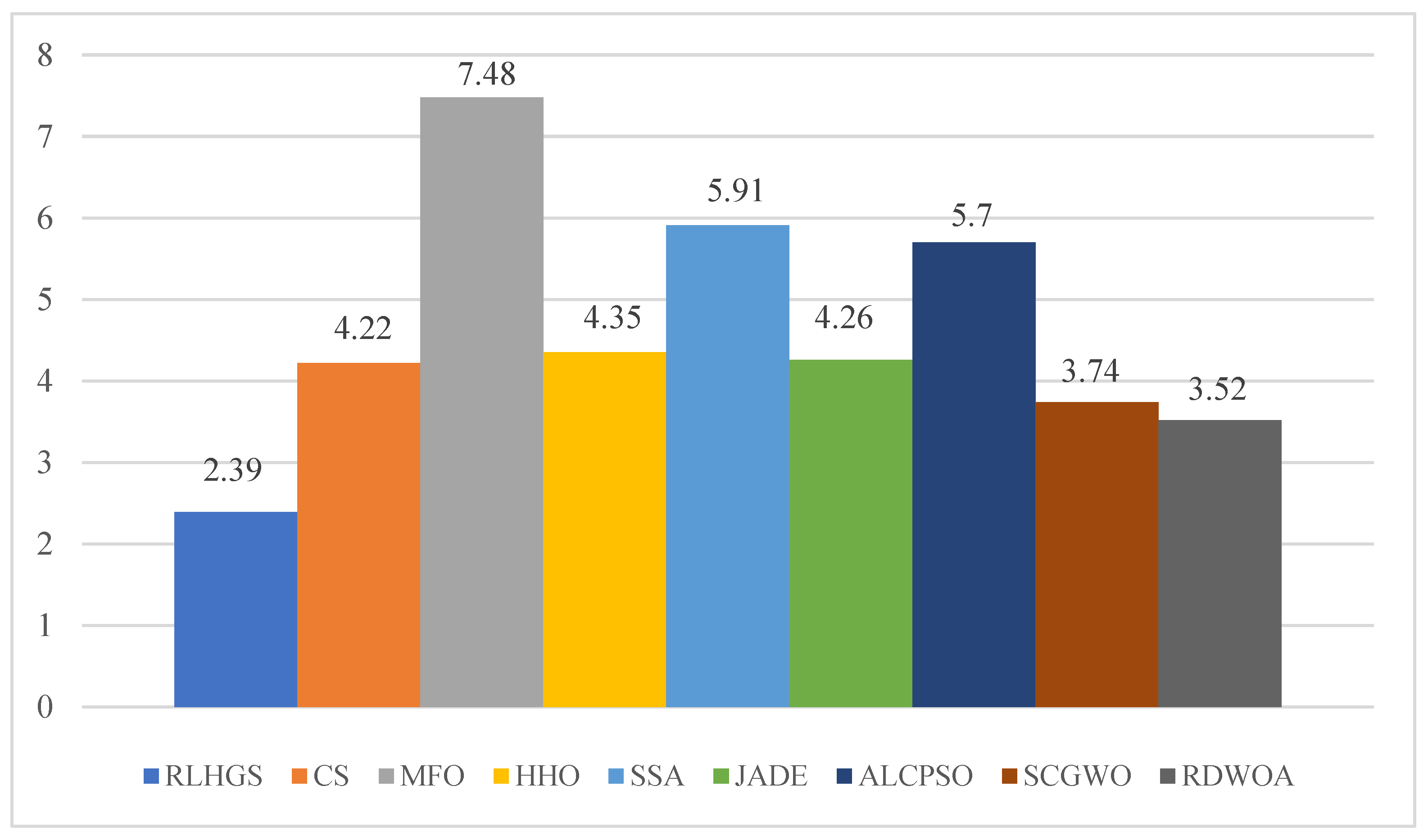
| RLHGS | CS | MFO | HHO | SSA | JADE | ALCPSO | SCGWO | RDWOA | |
|---|---|---|---|---|---|---|---|---|---|
| Average rank | 2.39 | 4.22 | 7.48 | 4.35 | 5.91 | 4.26 | 5.70 | 3.74 | 3.52 |
| Overall rank | 1 | 4 | 9 | 6 | 8 | 5 | 7 | 3 | 2 |
| CS | MFO | HHO | SSA | JADE | ALCPSO | SCGWO | RDWOA | |
|---|---|---|---|---|---|---|---|---|
| F1 | 1.7344 × 10⁻⁶ | 1.7333 × 10⁻⁶ | 1.0000 × 100 | 1.7333 × 10⁻⁶ | 1.7344 × 10⁻⁶ | 1.7344 × 10⁻⁶ | 1.0000 × 100 | 1.0000 × 100 |
| F2 | 4.3205 × 10⁻⁸ | 1.7344 × 10⁻⁶ | 1.0000 × 100 | 1.7344 × 10⁻⁶ | 1.7344 × 10⁻⁶ | 1.7344 × 10⁻⁶ | 1.2500 × 10⁻¹ | 1.0000 × 100 |
| F3 | 1.7344 × 10⁻⁶ | 1.7344 × 10⁻⁶ | 3.9063 × 10⁻³ | 1.7344 × 10⁻⁶ | 3.1123 × 10⁻⁵ | 1.7344 × 10⁻⁶ | 3.9063 × 10⁻³ | 3.9063 × 10⁻³ |
| F4 | 1.7344 × 10⁻⁶ | 1.7344 × 10⁻⁶ | 3.7896 × 10⁻⁶ | 1.7344 × 10⁻⁶ | 1.7344 × 10⁻⁶ | 1.7344 × 10⁻⁶ | 3.7896 × 10⁻⁶ | 3.7896 × 10⁻⁶ |
| F5 | 1.7344 × 10⁻⁶ | 1.7344 × 10⁻⁶ | 1.9209 × 10⁻⁶ | 1.9209 × 10⁻⁶ | 3.0861 × 10⁻¹ | 1.7344 × 10⁻⁶ | 1.7344 × 10⁻⁶ | 9.3157 × 10⁻⁶ |
| F6 | 1.7344 × 10⁻⁶ | 1.7333 × 10⁻⁶ | 1.7344 × 10⁻⁶ | 1.7344 × 10⁻⁶ | 1.7333 × 10⁻⁶ | 3.7243 × 10⁻⁵ | 1.7344 × 10⁻⁶ | 1.7344 × 10⁻⁶ |
| F7 | 2.3534 × 10⁻⁶ | 1.7344 × 10⁻⁶ | 1.7344 × 10⁻⁶ | 1.2453 × 10⁻² | 4.5281 × 10⁻¹ | 1.7344 × 10⁻⁶ | 1.7344 × 10⁻⁶ | 1.9209 × 10⁻⁶ |
| F8 | 3.1123 × 10⁻⁵ | 1.9729 × 10⁻⁵ | 4.4919 × 10⁻² | 3.1123 × 10⁻⁵ | 1.0201 × 10⁻¹ | 1.0570 × 10⁻⁴ | 5.7064 × 10⁻⁴ | 6.0350 × 10⁻³ |
| F9 | 1.7344 × 10⁻⁶ | 1.7344 × 10⁻⁶ | 1.0000 × 100 | 1.7344 × 10⁻⁶ | 7.8125 × 10⁻³ | 1.7344 × 10⁻⁶ | 1.0000 × 100 | 1.0000 × 100 |
| F10 | 1.7344 × 10⁻⁶ | 1.7344 × 10⁻⁶ | 1.0000 × 100 | 1.7344 × 10⁻⁶ | 1.7344 × 10⁻⁶ | 1.7344 × 10⁻⁶ | 1.0000 × 100 | 1.0000 × 100 |
| F11 | 4.9498 × 10⁻² | 3.5876 × 10⁻⁴ | 6.2500 × 10⁻² | 4.0702 × 10⁻² | 3.6811 × 10⁻² | 1.4793 × 10⁻² | 6.2500 × 10⁻² | 6.2500 × 10⁻² |
| F12 | 1.7344 × 10⁻⁶ | 1.7344 × 10⁻⁶ | 1.7344 × 10⁻⁶ | 1.7344 × 10⁻⁶ | 1.1499 × 10⁻⁴ | 1.7344 × 10⁻⁶ | 1.7344 × 10⁻⁶ | 1.7344 × 10⁻⁶ |
| F13 | 1.7344 × 10⁻⁶ | 1.7344 × 10⁻⁶ | 1.7344 × 10⁻⁶ | 1.7344 × 10⁻⁶ | 2.0589 × 10⁻¹ | 1.9209 × 10⁻⁶ | 1.9209 × 10⁻⁶ | 1.7344 × 10⁻⁶ |
| F14 | 1.0000 × 100 | 4.8828 × 10⁻⁴ | 1.7344 × 10⁻⁶ | 1.0000 × 100 | 1.0000 × 100 | 1.0000 × 100 | 1.7213 × 10⁻⁶ | 1.5625 × 10⁻² |
| F15 | 8.4303 × 10⁻⁶ | 1.7257 × 10⁻⁶ | 3.1123 × 10⁻⁵ | 1.0246 × 10⁻⁵ | 2.2513 × 10⁻² | 1.7372 × 10⁻¹ | 3.1123 × 10⁻⁵ | 3.1123 × 10⁻⁵ |
| F16 | 1.0000 × 100 | 1.0000 × 100 | 4.8828 × 10⁻⁴ | 2.2090 × 10⁻⁵ | 1.0000 × 100 | 1.0000 × 100 | 1.7344 × 10⁻⁶ | 1.0000 × 100 |
| F17 | 1.0000 × 100 | 1.0000 × 100 | 4.0100 × 10⁻⁵ | 1.2500 × 10⁻¹ | 1.0000 × 100 | 1.0000 × 100 | 1.7344 × 10⁻⁶ | 4.8828 × 10⁻⁴ |
| F18 | 5.7330 × 10⁻⁷ | 1.6244 × 10⁻⁴ | 1.6837 × 10⁻⁶ | 1.5871 × 10⁻⁶ | 3.4375 × 10⁻¹ | 6.1035 × 10⁻⁵ | 1.7344 × 10⁻⁶ | 1.4307 × 10⁻¹ |
| F19 | 1.0000 × 100 | 1.0000 × 100 | 1.7344 × 10⁻⁶ | 1.2207 × 10⁻⁴ | 1.0000 × 100 | 1.0000 × 100 | 1.7344 × 10⁻⁶ | 1.2500 × 10⁻¹ |
| F20 | 1.0000 × 100 | 4.3895 × 10⁻⁵ | 1.7344 × 10⁻⁶ | 1.7322 × 10⁻⁶ | 7.8125 × 10⁻³ | 4.8828 × 10⁻⁴ | 1.7344 × 10⁻⁶ | 9.7656 × 10⁻⁴ |
| F21 | 1.0000 × 100 | 4.8828 × 10⁻⁴ | 1.7344 × 10⁻⁶ | 1.7333 × 10⁻⁶ | 1.5625 × 10⁻² | 7.8125 × 10⁻³ | 1.7344 × 10⁻⁶ | 5.0000 × 10⁻¹ |
| F22 | 1.0000 × 100 | 7.8125 × 10⁻³ | 1.7344 × 10⁻⁶ | 1.7344 × 10⁻⁶ | 2.5000 × 10⁻¹ | 6.2500 × 10⁻² | 1.7344 × 10⁻⁶ | 1.2500 × 10⁻¹ |
| F23 | 1.0000 × 100 | 2.4414 × 10⁻⁴ | 1.7344 × 10⁻⁶ | 1.7322 × 10⁻⁶ | 2.5000 × 10⁻¹ | 2.5000 × 10⁻¹ | 1.7344 × 10⁻⁶ | 1.2500 × 10⁻¹ |
| RLHGS | CS | MFO | HHO | SSA | JADE | ALCPSO | SCGWO | RDWOA | |
|---|---|---|---|---|---|---|---|---|---|
| F1 | 8.4691 × 10² | 2.0354 × 100 | 1.4498 × 100 | 1.4526 × 100 | 1.2668 × 100 | 1.6710 × 101 | 8.3820 × 10⁻¹ | 1.9997 × 100 | 1.0154 × 100 |
| F2 | 3.0396 × 10² | 2.0626 × 100 | 1.5539 × 100 | 1.2214 × 100 | 1.1745 × 100 | 1.6865 × 101 | 7.9440 × 10⁻¹ | 1.1329 × 101 | 8.6280 × 10⁻¹ |
| F3 | 2.0991 × 10³ | 4.2184 × 100 | 3.6022 × 100 | 3.8757 × 100 | 3.6416 × 100 | 1.6792 × 101 | 2.9570 × 100 | 4.5626 × 100 | 3.4932 × 100 |
| F4 | 7.0378 × 100 | 1.9587 × 100 | 1.4081 × 100 | 1.1868 × 100 | 1.1103 × 100 | 1.6182 × 101 | 7.3280 × 10⁻¹ | 1.9553 × 100 | 9.5240 × 10⁻¹ |
| F5 | 4.4681 × 100 | 2.2221 × 100 | 1.6676 × 100 | 1.5862 × 100 | 1.4441 × 100 | 1.2135 × 101 | 1.0096 × 100 | 2.1779 × 100 | 1.0915 × 100 |
| F6 | 9.6883 × 100 | 1.9612 × 100 | 1.3927 × 100 | 1.2491 × 100 | 1.1359 × 100 | 1.3613 × 101 | 7.6700 × 10⁻¹ | 1.8489 × 100 | 7.8840 × 10⁻¹ |
| F7 | 8.3248 × 100 | 3.1648 × 100 | 2.6076 × 100 | 2.4620 × 100 | 2.4082 × 100 | 1.3690 × 101 | 1.9893 × 100 | 3.1472 × 100 | 2.0583 × 100 |
| F8 | 1.5842 × 101 | 2.4678 × 100 | 1.6926 × 100 | 1.6836 × 100 | 1.4959 × 100 | 1.2785 × 101 | 1.0662 × 100 | 2.2461 × 100 | 1.1192 × 100 |
| F9 | 9.9402 × 100 | 2.1947 × 100 | 1.6374 × 100 | 1.4256 × 100 | 1.3468 × 100 | 1.3356 × 101 | 9.2490 × 10⁻¹ | 1.9687 × 100 | 8.8810 × 10⁻¹ |
| F10 | 1.9390 × 10³ | 2.1445 × 100 | 1.5712 × 100 | 1.4695 × 100 | 1.3655 × 100 | 1.3987 × 101 | 1.0166 × 100 | 1.9999 × 100 | 8.9220 × 10⁻¹ |
| F11 | 2.0717 × 101 | 2.2916 × 100 | 1.9069 × 100 | 1.6695 × 100 | 1.6033 × 100 | 1.4202 × 101 | 1.2030 × 100 | 2.2250 × 100 | 1.1195 × 100 |
| F12 | 9.4747 × 101 | 5.3738 × 100 | 4.9777 × 100 | 5.0041 × 100 | 4.8790 × 100 | 1.3993 × 101 | 4.3605 × 100 | 5.5637 × 100 | 4.4780 × 100 |
| F13 | 9.8841 × 101 | 5.3597 × 100 | 4.8539 × 100 | 4.9606 × 100 | 4.9572 × 100 | 1.4223 × 101 | 4.2401 × 100 | 5.5618 × 100 | 4.4716 × 100 |
| F14 | 1.5509 × 101 | 7.4750 × 100 | 7.0009 × 100 | 7.9889 × 100 | 7.4952 × 100 | 1.5530 × 101 | 7.0055 × 100 | 7.4837 × 100 | 7.2453 × 100 |
| F15 | 1.0824 × 100 | 1.3539 × 100 | 7.2870 × 10⁻¹ | 9.9650 × 10⁻¹ | 7.6850 × 10⁻¹ | 1.4078 × 101 | 5.9570 × 10⁻¹ | 7.4800 × 10⁻¹ | 5.1670 × 10⁻¹ |
| F16 | 9.1510 × 10⁻¹ | 1.2614 × 100 | 6.7380 × 10⁻¹ | 9.9940 × 10⁻¹ | 7.5030 × 10⁻¹ | 1.4111 × 101 | 5.6660 × 10⁻¹ | 6.8380 × 10⁻¹ | 4.9330 × 10⁻¹ |
| F17 | 7.1150 × 10⁻¹ | 1.2121 × 100 | 6.0240 × 10⁻¹ | 9.1370 × 10⁻¹ | 1.0718 × 100 | 1.4722 × 101 | 4.7700 × 10⁻¹ | 6.1810 × 10⁻¹ | 4.1870 × 10⁻¹ |
| F18 | 6.8490 × 10⁻¹ | 1.1509 × 100 | 5.5690 × 10⁻¹ | 8.8080 × 10⁻¹ | 6.1910 × 10⁻¹ | 1.4674 × 101 | 4.6230 × 10⁻¹ | 5.6180 × 10⁻¹ | 3.8660 × 10⁻¹ |
| F19 | 1.4690 × 100 | 1.3812 × 100 | 7.9660 × 10⁻¹ | 1.1445 × 100 | 8.4850 × 10⁻¹ | 1.4617 × 101 | 6.9460 × 10⁻¹ | 8.3090 × 10⁻¹ | 6.0620 × 10⁻¹ |
| F20 | 2.2828 × 100 | 1.4905 × 100 | 8.9780 × 10⁻¹ | 1.1964 × 100 | 8.6360 × 10⁻¹ | 1.4959 × 101 | 7.2180 × 10⁻¹ | 9.7150 × 10⁻¹ | 6.4140 × 10⁻¹ |
| F21 | 2.2604 × 100 | 1.6074 × 100 | 1.0257 × 100 | 1.4272 × 100 | 1.1057 × 100 | 1.4296 × 101 | 9.0980 × 10⁻¹ | 1.0835 × 100 | 8.2640 × 10⁻¹ |
| F22 | 3.3694 × 100 | 1.7528 × 100 | 1.1738 × 100 | 1.5229 × 100 | 1.2353 × 100 | 1.4679 × 101 | 1.0392 × 100 | 1.2358 × 100 | 9.6330 × 10⁻¹ |
| F23 | 3.9384 × 100 | 1.9808 × 100 | 1.3808 × 100 | 1.6951 × 100 | 1.4924 × 100 | 1.4746 × 101 | 1.2949 × 100 | 1.4418 × 100 | 1.1654 × 100 |
| F1 | F2 | F3 | |||||||
| Avg | Std | Rank | Avg | Std | Rank | Avg | Std | Rank | |
| RLHGS | 2.8842 × 10⁴ | 3.1972 × 10⁴ | 2 | 8.4538 × 10³ | 6.5144 × 10² | 1 | 1.0688 × 10³ | 3.3354 × 101 | 1 |
| CS | 1.0000 × 10¹⁰ | 0.0000 × 100 | 7 | 2.0238 × 10⁴ | 4.8058 × 10² | 7 | 2.5278 × 10³ | 1.8830 × 10² | 5 |
| MFO | 1.5398 × 10¹¹ | 5.0361 × 10¹⁰ | 9 | 1.7701 × 10⁴ | 2.1140 × 10³ | 5 | 5.2734 × 10³ | 1.2197 × 10³ | 9 |
| HHO | 4.2402 × 10⁸ | 5.1004 × 10⁷ | 5 | 1.9801 × 10⁴ | 1.6613 × 10³ | 6 | 4.2440 × 10³ | 2.2379 × 10² | 8 |
| SSA | 3.3528 × 10⁴ | 3.0298 × 10⁴ | 3 | 1.6415 × 10⁴ | 1.7661 × 10³ | 4 | 1.8667 × 10³ | 1.7702 × 10² | 3 |
| JADE | 3.5454 × 10³ | 6.0412 × 10³ | 1 | 1.2316 × 10⁴ | 6.0211 × 10² | 2 | 1.3513 × 10³ | 1.0439 × 10² | 2 |
| ALCPSO | 7.0851 × 10⁵ | 2.5719 × 10⁶ | 4 | 1.5905 × 10⁴ | 1.8514 × 10³ | 3 | 2.0011 × 10³ | 2.5319 × 10² | 4 |
| SCGWO | 5.2861 × 10¹⁰ | 9.9659 × 10⁹ | 8 | 2.4465 × 10⁴ | 2.7615 × 10³ | 9 | 2.9184 × 10³ | 2.4402 × 10² | 6 |
| RDWOA | 2.5547 × 10⁹ | 2.4393 × 10⁹ | 6 | 2.0553 × 10⁴ | 2.6338 × 10³ | 8 | 3.4061 × 10³ | 2.5938 × 10² | 7 |
| F4 | F5 | F6 | |||||||
| Avg | Std | Rank | Avg | Std | Rank | Avg | Std | Rank | |
| RLHGS | 3.1514 × 10³ | 3.3690 × 10² | 1 | 1.9036 × 10⁶ | 7.1206 × 10⁵ | 2 | 3.6308 × 10³ | 3.5935 × 10² | 1 |
| CS | 4.9160 × 10³ | 1.8578 × 10² | 4 | 5.6825 × 10⁶ | 1.1166 × 10⁶ | 4 | 7.0747 × 10³ | 2.9911 × 10² | 5 |
| MFO | 5.9846 × 10³ | 6.5043 × 10² | 7 | 4.8669 × 10⁷ | 4.5316 × 10⁷ | 8 | 9.3841 × 10³ | 1.9076 × 10³ | 8 |
| HHO | 6.1115 × 10³ | 6.6172 × 10² | 8 | 1.8198 × 10⁷ | 5.6157 × 10⁶ | 6 | 8.7679 × 10³ | 9.6870 × 10² | 7 |
| SSA | 4.9150 × 10³ | 4.9846 × 10² | 3 | 1.9370 × 10⁶ | 6.8365 × 10⁵ | 3 | 6.6963 × 10³ | 8.9749 × 10² | 4 |
| JADE | 3.9526 × 10³ | 3.3609 × 10² | 2 | 1.0424 × 10⁵ | 7.2950 × 10⁴ | 1 | 4.8052 × 10³ | 3.6056 × 10² | 2 |
| ALCPSO | 5.1273 × 10³ | 5.7647 × 10² | 5 | 2.0526 × 10⁷ | 1.3196 × 10⁷ | 7 | 5.9489 × 10³ | 6.3801 × 10² | 3 |
| SCGWO | 5.6881 × 10³ | 8.3109 × 10² | 6 | 8.5044 × 10⁷ | 3.3393 × 10⁷ | 9 | 1.0681 × 10⁴ | 9.6922 × 10² | 9 |
| RDWOA | 6.2967 × 10³ | 8.4208 × 10² | 9 | 1.7386 × 10⁷ | 1.0132 × 10⁷ | 5 | 8.6443 × 10³ | 1.0865 × 10³ | 6 |
| F7 | F8 | F9 | |||||||
| Avg | Std | Rank | Avg | Std | Rank | Avg | Std | Rank | |
| RLHGS | 1.3633 × 10⁶ | 7.1889 × 10⁵ | 2 | 2.3500 × 10³ | 2.0959 × 10⁻¹² | 4 | 2.6883 × 10³ | 4.8347 × 10² | 5 |
| CS | 2.8415 × 10⁶ | 5.9766 × 10⁵ | 4 | 2.3500 × 10³ | 7.6080 × 10⁻⁹ | 7 | 3.5166 × 10³ | 1.1805 × 10³ | 7 |
| MFO | 2.8668 × 10⁷ | 3.3622 × 10⁷ | 9 | 2.3539 × 10³ | 2.6837 × 100 | 9 | 6.2667 × 10³ | 1.7959 × 10² | 9 |
| HHO | 8.5364 × 10⁶ | 2.7549 × 10⁶ | 7 | 2.3500 × 10³ | 1.8501 × 10⁻¹² | 1 | 2.6000 × 10³ | 0.0000 × 100 | 1 |
| SSA | 1.7033 × 10⁶ | 7.0658 × 10⁵ | 3 | 2.3500 × 10³ | 5.2391 × 10⁻¹⁰ | 6 | 2.6006 × 10³ | 1.8723 × 100 | 4 |
| JADE | 3.4821 × 10⁴ | 1.4681 × 10⁴ | 1 | 2.3500 × 10³ | 2.5461 × 10⁻¹¹ | 5 | 2.7754 × 10³ | 6.7185 × 10² | 6 |
| ALCPSO | 6.4144 × 10⁶ | 5.2462 × 10⁶ | 5 | 2.3500 × 10³ | 9.2761 × 10−07 | 8 | 5.9265 × 10³ | 7.2027 × 10² | 8 |
| SCGWO | 2.5290 × 10⁷ | 1.0245 × 10⁷ | 8 | 2.3500 × 10³ | 1.8501 × 10⁻¹² | 1 | 2.6000 × 10³ | 0.0000 × 100 | 1 |
| RDWOA | 6.7465 × 10⁶ | 3.3014 × 10⁶ | 6 | 2.3500 × 10³ | 1.8501 × 10⁻¹² | 1 | 2.6000 × 10³ | 0.0000 × 100 | 1 |
| F10 | |||||||||
| Avg | Std | Rank | +/−/= | ||||||
| RLHGS | 3.0507 × 10³ | 1.6231 × 10² | 4 | ~ | |||||
| CS | 3.3320 × 10³ | 4.8669 × 101 | 6 | 10/0/0 | |||||
| MFO | 1.1700 × 10⁴ | 5.5656 × 10³ | 9 | 10/0/0 | |||||
| HHO | 2.7000 × 10³ | 0.0000 × 100 | 1 | 7/1/2 | |||||
| SSA | 3.3086 × 10³ | 7.1568 × 101 | 5 | 6/1/3 | |||||
| JADE | 3.3464 × 10³ | 7.4316 × 101 | 7 | 7/3/0 | |||||
| ALCPSO | 3.4605 × 10³ | 1.3361 × 10² | 8 | 9/0/1 | |||||
| SCGWO | 2.7000 × 10³ | 0.0000 × 100 | 1 | 7/1/2 | |||||
| RDWOA | 2.7000 × 10³ | 0.0000 × 100 | 1 | 7/1/2 |
| RLHGS | CS | MFO | HHO | SSA | JADE | ALCPSO | SCGWO | RDWOA | |
|---|---|---|---|---|---|---|---|---|---|
| Average rank | 2.3 | 5.6 | 8.2 | 5.0 | 3.8 | 2.9 | 5.5 | 5.8 | 5.0 |
| Overall rank | 1 | 7 | 9 | 4 | 3 | 2 | 6 | 8 | 4 |
| CS | MFO | HHO | SSA | JADE | ALCPSO | SCGWO | RDWOA | |
|---|---|---|---|---|---|---|---|---|
| F1 | 1.7344 × 10⁻⁶ | 1.7344 × 10⁻⁶ | 1.7344 × 10⁻⁶ | 5.3044 × 10⁻¹ | 2.5967 × 10⁻⁵ | 2.6230 × 10⁻¹ | 1.7344 × 10⁻⁶ | 1.7344 × 10⁻⁶ |
| F2 | 1.7344 × 10⁻⁶ | 1.7344 × 10⁻⁶ | 1.7344 × 10⁻⁶ | 1.7344 × 10⁻⁶ | 1.7344 × 10⁻⁶ | 1.7344 × 10⁻⁶ | 1.7344 × 10⁻⁶ | 1.7344 × 10⁻⁶ |
| F3 | 1.7344 × 10⁻⁶ | 1.7344 × 10⁻⁶ | 1.7344 × 10⁻⁶ | 1.7344 × 10⁻⁶ | 1.7344 × 10⁻⁶ | 1.7344 × 10⁻⁶ | 1.7344 × 10⁻⁶ | 1.7344 × 10⁻⁶ |
| F4 | 1.7344 × 10⁻⁶ | 1.7344 × 10⁻⁶ | 1.7344 × 10⁻⁶ | 1.7344 × 10⁻⁶ | 3.8822 × 10⁻⁶ | 1.7344 × 10⁻⁶ | 1.7344 × 10⁻⁶ | 1.7344 × 10⁻⁶ |
| F5 | 1.7344 × 10⁻⁶ | 1.7344 × 10⁻⁶ | 1.7344 × 10⁻⁶ | 7.9710 × 10⁻¹ | 1.7344 × 10⁻⁶ | 1.7344 × 10⁻⁶ | 1.7344 × 10⁻⁶ | 1.7344 × 10⁻⁶ |
| F6 | 1.7344 × 10⁻⁶ | 1.7344 × 10⁻⁶ | 1.7344 × 10⁻⁶ | 1.7344 × 10⁻⁶ | 1.7344 × 10⁻⁶ | 1.7344 × 10⁻⁶ | 1.7344 × 10⁻⁶ | 1.7344 × 10⁻⁶ |
| F7 | 3.1817 × 10⁻⁶ | 1.7344 × 10⁻⁶ | 1.7344 × 10⁻⁶ | 1.2044 × 10⁻¹ | 1.7344 × 10⁻⁶ | 2.3534 × 10⁻⁶ | 1.7344 × 10⁻⁶ | 1.7344 × 10⁻⁶ |
| F8 | 1.7344 × 10⁻⁶ | 1.7344 × 10⁻⁶ | 6.2500 × 10⁻² | 1.7344 × 10⁻⁶ | 2.6114 × 10⁻⁷ | 1.1123 × 10⁻⁶ | 6.2500 × 10⁻² | 6.2500 × 10⁻² |
| F9 | 1.9729 × 10⁻⁵ | 1.7344 × 10⁻⁶ | 1.0000 × 100 | 3.1123 × 10⁻⁵ | 2.6770 × 10⁻⁵ | 1.7344 × 10⁻⁶ | 1.0000 × 100 | 1.0000 × 100 |
| F10 | 1.7344 × 10⁻⁶ | 1.7344 × 10⁻⁶ | 1.2290 × 10⁻⁵ | 1.7344 × 10⁻⁶ | 1.7344 × 10⁻⁶ | 1.7344 × 10⁻⁶ | 1.2290 × 10⁻⁵ | 1.2290 × 10⁻⁵ |
| MAs | Optimal Values of Parameters | Optimum Cost | ||
|---|---|---|---|---|
| RLHGS | 0.051749979 | 0.358185026 | 11.20345892 | 0.0126653 |
| IHS [100] | 0.051154 | 0.349871 | 12.076432 | 0.0126706 |
| MFO [93] | 0.053064 | 0.390718 | 9.542437 | 0.012699 |
| PSO [25] | 0.015728 | 0.357644 | 11.244543 | 0.0126747 |
| WOA [101] | 0.050451 | 0.327675 | 13.219341 | 0.012694 |
| GSA [33] | 0.050276 | 0.345215 | 13.52541 | 0.0126763 |
| INFO [36] | 0.051555 | 0.353499 | 11.48034 | 0.012666 |
| SMA [28] | 0.05847 | 0.523420486 | 6.95166221 | 0.0160198 |
| SMFO [102] | 0.06573 | 0.32869515 | 2.629561202 | 0.0138029 |
| MAs | Optimal Values of Parameters | Optimum Cost | |||
|---|---|---|---|---|---|
| RLHGS | 0.2015 | 3.3345 | 9.03662391 | 0.20572964 | 1.699986 |
| HGS [60] | 0.26 | 5.1025 | 8.03961 | 0.26 | 2.302076 |
| GSA [33] | 0.182129 | 3.856979 | 10 | 0.202376 | 1.879952 |
| CDE [41] | 0.203137 | 3.542998 | 9.033498 | 0.206179 | 1.733462 |
| HS [103] | 0.2442 | 6.2231 | 8.2915 | 0.2443 | 2.3807 |
| GWO [26] | 0.205676 | 3.478377 | 9.03681 | 0.205778 | 1.72624000 |
| BA [104] | 2 | 0.100000 | 3.174303 | 2 | 1.8181 |
| IHS [100] | 0.205730 | 3.470490 | 9.036620 | 0.20573 | 1.7248 |
| RO [105] | 0.203687 | 3.528467 | 9.004233 | 0.207241 | 1.735344 |
| SIMPLEX [106] | 0.2792 | 5.6256 | 7.7512 | 0.2796 | 2.5307 |
| MAs | Optimal Values of Parameters | Optimum Cost | |||
|---|---|---|---|---|---|
| RLHGS | 0.8125 | 0.4375 | 42.0984456 | 176.6365958 | 6059.714335 |
| ES [107] | 0.8125 | 0.4375 | 42.098087 | 176.640518 | 6059.7456 |
| PSO [25] | 0.8125 | 0.4375 | 42.091266 | 176.7465 | 6061.0777 |
| GA [22] | 0.9375 | 0.5 | 48.329 | 112.679 | 6410.3811 |
| G-QPSO [108] | 0.8125 | 0.4375 | 42.0984 | 176.6372 | 6059.7208 |
| SMA [28] | 0.75 | 50.3125 | 41.17 | 193.001 | 6772.7333 |
| Branch-and-bound [109] | 1.125 | 0.625 | 47.7 | 117.71 | 8129.1036 |
| IHS [100] | 1.125 | 0.625 | 58.29015 | 43.69268 | 7197.73 |
| GA3 [81] | 0.812500 | 0.437500 | 42.0974 | 176.6540 | 6059.9463 |
| CPSO [110] | 0.812500 | 0.437500 | 42.091266 | 176.746500 | 6061.0777 |
| MAs | Optimal Values of Parameters | Optimum Cost | |
|---|---|---|---|
| RLHGS | 0.788673486 | 0.408252954 | 263.89584338 |
| CS [92] | 0.78867 | 0.40902 | 263.9716 |
| MFO [93] | 0.788244771 | 0.409466958 | 263.8959797 |
| BWOA [98] | 0.788666327 | 0.408273202 | 263.8958435 |
| GOA [111] | 0.788897556 | 0.40761957 | 263.8958815 |
| MBA [112] | 0.7885650 | 0.4085597 | 263.8958522 |
| MVO [34] | 0.78860276 | 0.408453070 | 263.8958499 |
Disclaimer/Publisher’s Note: The statements, opinions and data contained in all publications are solely those of the individual author(s) and contributor(s) and not of MDPI and/or the editor(s). MDPI and/or the editor(s) disclaim responsibility for any injury to people or property resulting from any ideas, methods, instructions or products referred to in the content. |
© 2023 by the authors. Licensee MDPI, Basel, Switzerland. This article is an open access article distributed under the terms and conditions of the Creative Commons Attribution (CC BY) license (https://creativecommons.org/licenses/by/4.0/).
Share and Cite
Lin, Y.; Heidari, A.A.; Wang, S.; Chen, H.; Zhang, Y. An Enhanced Hunger Games Search Optimization with Application to Constrained Engineering Optimization Problems. Biomimetics 2023, 8, 441. https://doi.org/10.3390/biomimetics8050441
Lin Y, Heidari AA, Wang S, Chen H, Zhang Y. An Enhanced Hunger Games Search Optimization with Application to Constrained Engineering Optimization Problems. Biomimetics. 2023; 8(5):441. https://doi.org/10.3390/biomimetics8050441
Chicago/Turabian StyleLin, Yaoyao, Ali Asghar Heidari, Shuihua Wang, Huiling Chen, and Yudong Zhang. 2023. "An Enhanced Hunger Games Search Optimization with Application to Constrained Engineering Optimization Problems" Biomimetics 8, no. 5: 441. https://doi.org/10.3390/biomimetics8050441