


A Novel Bio-Inspired Optimization Algorithm Design for Wind Power Engineering Applications Time-Series Forecasting

 ,
,
Abstract
:1. Introduction
- Providing machine learning-based methodologies to Wind Power time-series forecasting.
- Introducing the optimization-based Recurrent Neural Network (RNN) forecasting model incorporating a Dynamic Fitness Al-Biruni Earth Radius (DFBER) algorithm to predict the wind power data patterns.
- Currently developing an optimized RNN-DFBER-based regression model to enhance the accuracy of predictions using the evaluated dataset.
- Conducting a comparison among different algorithms to determine which one yields the most favorable outcomes.
- Employing Wilcoxon rank-sum and ANOVA tests to assess the potential statistical significance of the optimized RNN-DFBER-based model.
- The RNN-DFBER-based regression model’s flexibility allows it to be tested and customized for various datasets, thanks to its adaptability.
2. Materials and Methods
2.1. Recurrent Neural Network
2.2. Al-Biruni Earth Radius (BER) Algorithm
| Algorithm 1: AL-Biruni Earth Radius (BER) algorithm |
| 1: Initialize BER population and parameters, 2: Calculate objective function for each agent 3: Find best agent 4: while do 5: for () do 6: Update , 7: Move to best agent as in Equation (1) 8: end for 9: for () do 10: Update , 11: Elitism of the best agent as in Equation (2) 12: Investigating area around best agent as in Equation (3) 13: Select best agent by comparing and 14: if The best fitness value with no change for two iterations. then 15: Mutate solution as in Equation (4) 16: end if 17: end for 18: Update objective function for each agent 19: Find best agent as 20: Update BER parameters, 21: end while 22: Return best agent |
3. Proposed Dynamic Fitness BER Algorithm
| Algorithm 2: The proposed DFBER algorithm |
| 1: Initialize population and parameters, 2: Calculate fitness function for each agent 3: Find first, second, and third best agents 4: while do 5: if (For three iterations, the best fitness value is the same) then 6: Increase agents in exploration group 7: Decrease agents in exploitation group 8: end if 9: for () do 10: Update , 11: Update positions of agents as 12: end for 13: for () do 14: Update r = h , 15: Update Fitness 16: Update Fitness 17: Update Fitness 18: Calculate 19: Elitism of the best agent as 20: Investigating area around best agent as 21: Select best agent by comparing and 22: if The best fitness value with no change for two iterations. then 23: Mutate solution as 24: end if 25: end for 26: Update fitness function for each agent 27: Find best three agents 28: Set first best agent as 29: Update parameters, 30: end while 31: Return best agent |
3.1. Motivation
3.2. Dynamic Feature of DFBER Algorithm
3.3. Fitness Al-Biruni Earth Radius Algorithm
3.4. Complexity Analysis
- Initialize population and parameters, .
- Calculate fitness function for each agent: .
- Finding best three solutions: .
- Updating agents in exploration and exploitation groups: .
- Updating position of current agents in exploration group: .
- Updating position of current agents in exploitation group by fitness functions: .
- Updating fitness function for each agent: .
- Finding best fitness: .
- Finding best three solutions: .
- Set first best agent as : .
- Updating parameters: .
- Updating iterations: .
- Return the best fitness: .
3.5. Fitness Function
4. Experimental Results
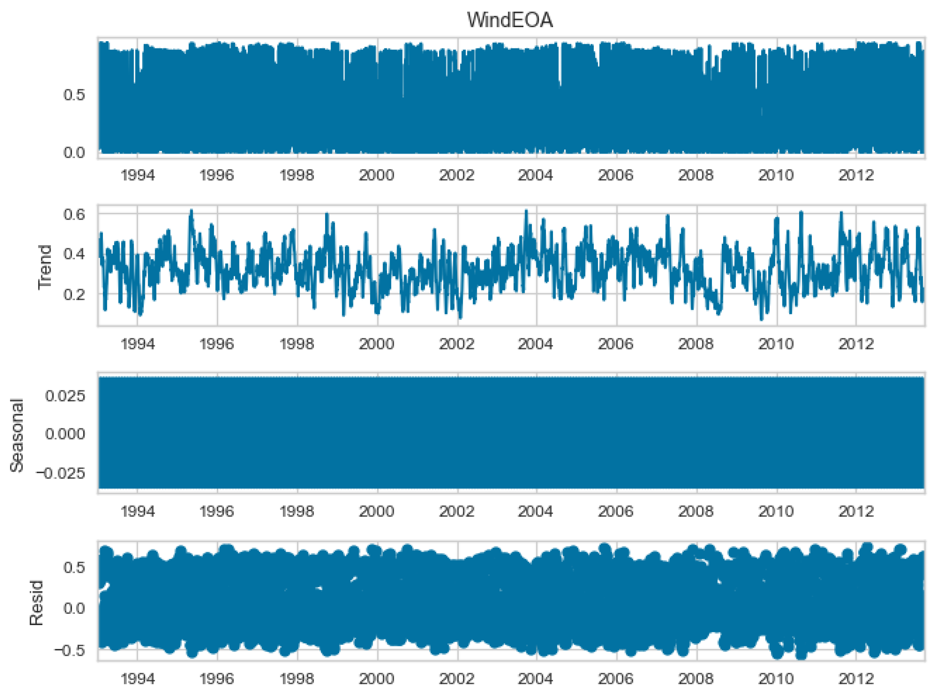
4.1. Dataset
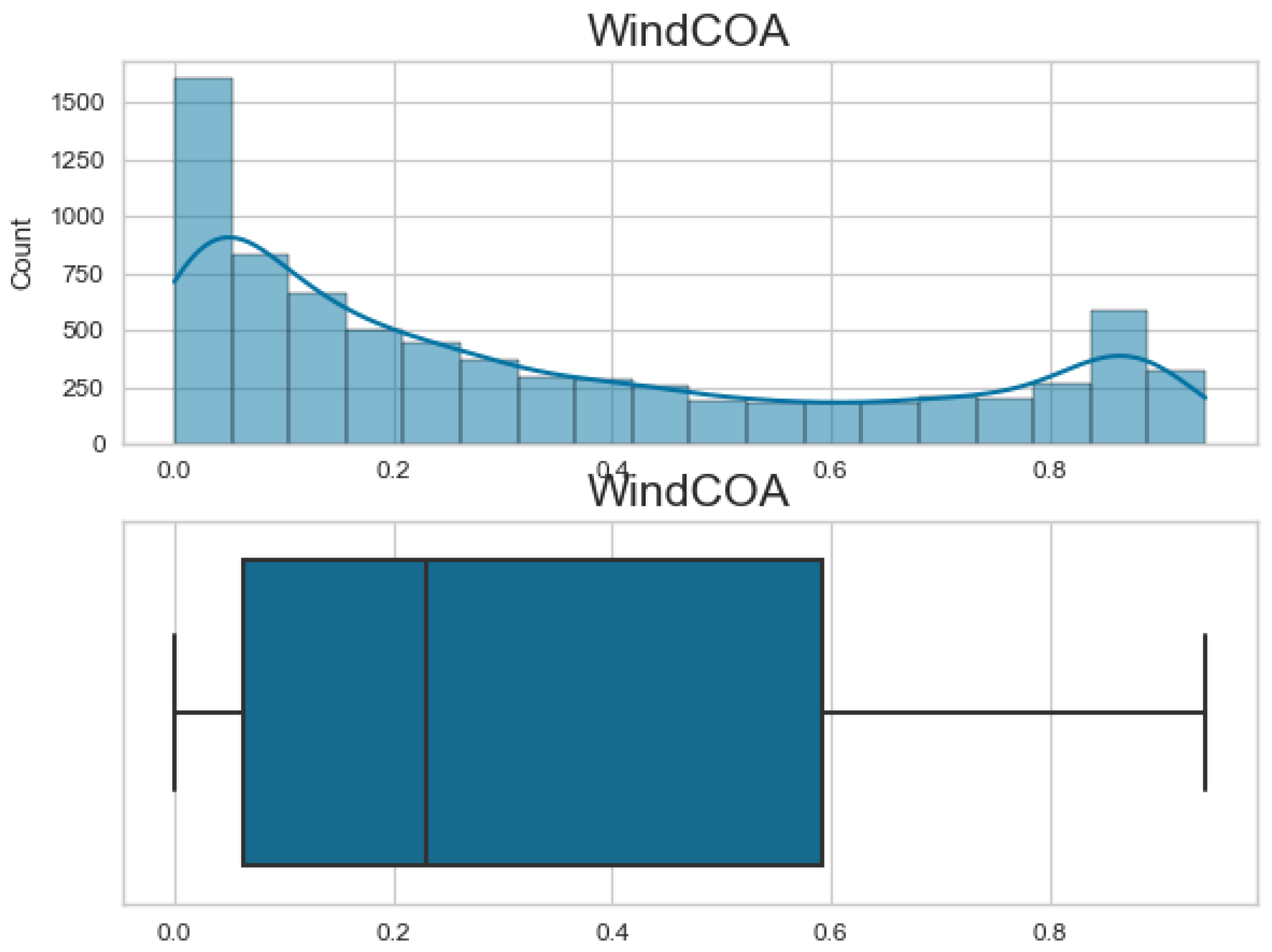
- Central Operating Area (COA): This refers to a specific region or area where the central energy generation operations occur.
- Eastern Operating Area (EOA): This refers to a specific region or area where energy generation operations are concentrated in the eastern part.
- Southern Operating Area (SOA): This refers to a specific region or area where energy generation operations are concentrated in the southern part.
- Western Operating Area (WOA): This refers to a specific region or area where energy generation operations are concentrated in the western part.
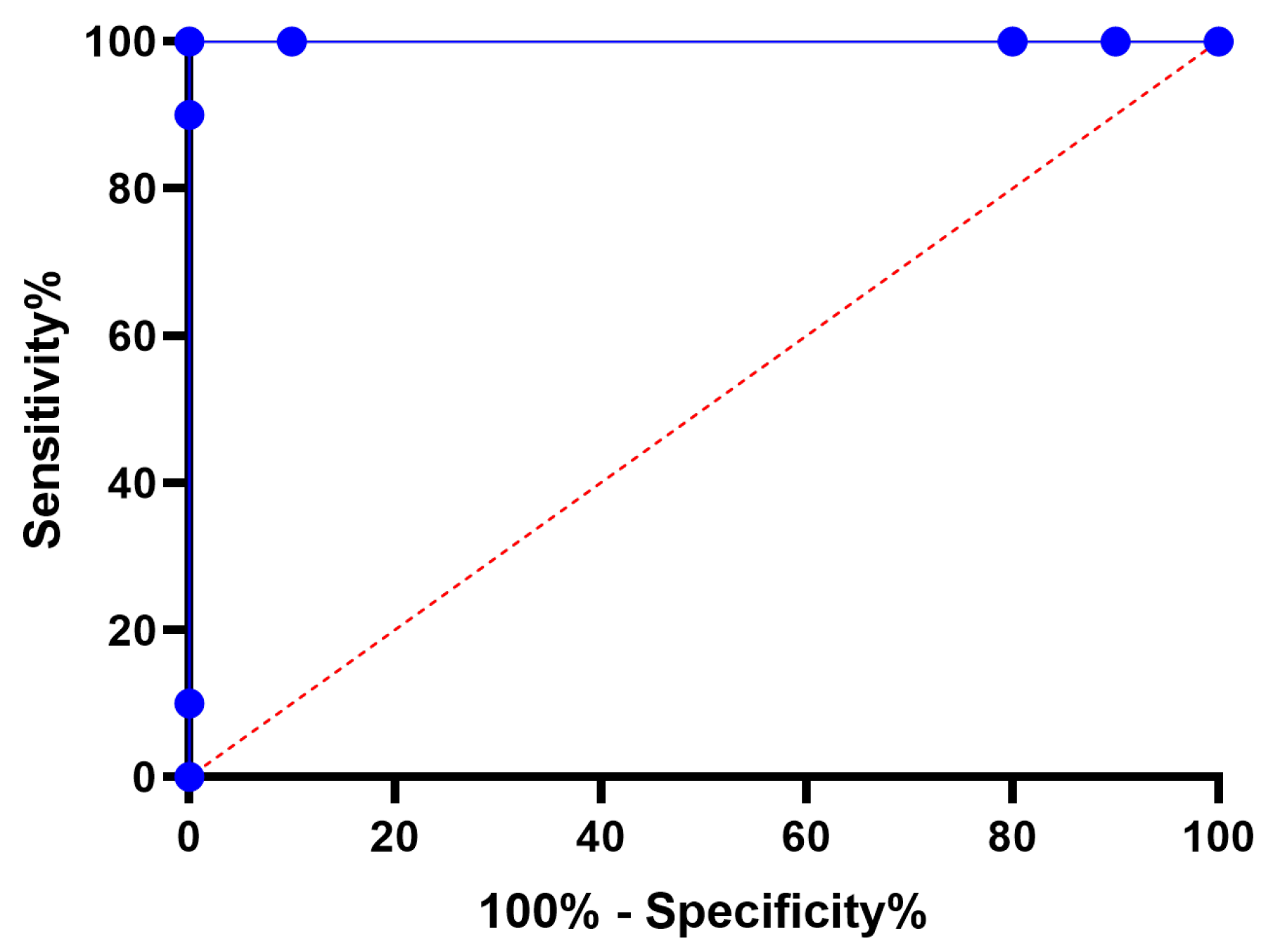
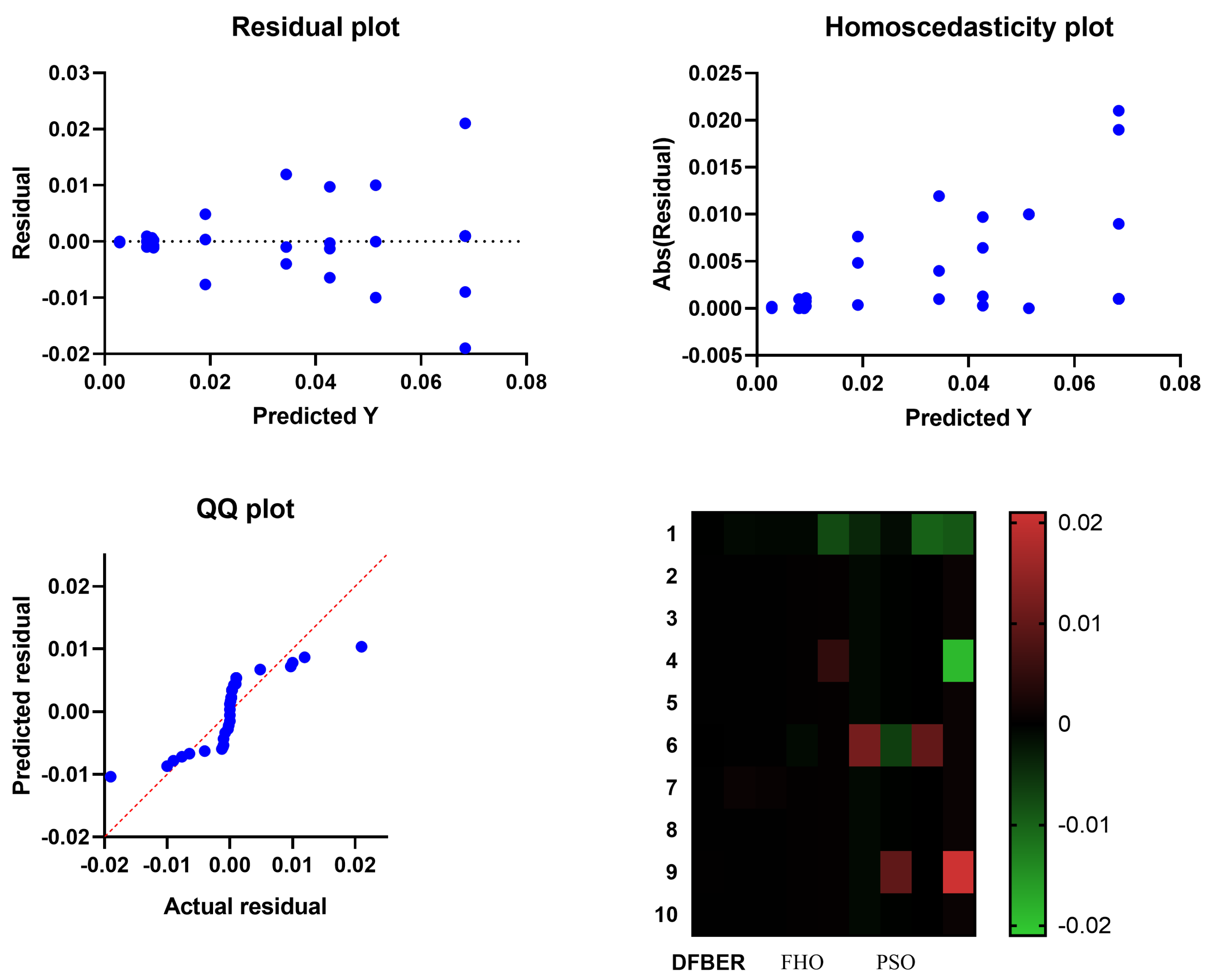
4.2. Regression Results and Discussions
5. Discussion
6. Conclusions and Future Work
Author Contributions
Funding
Institutional Review Board Statement
Data Availability Statement
Acknowledgments
Conflicts of Interest
References
- Valdivia-Bautista, S.M.; Domínguez-Navarro, J.A.; Pérez-Cisneros, M.; Vega-Gómez, C.J.; Castillo-Téllez, B. Artificial Intelligence in Wind Speed Forecasting: A Review. Energies 2023, 16, 2457. [Google Scholar] [CrossRef]
- Ibrahim, A.; El-kenawy, E.S.M.; Kabeel, A.E.; Karim, F.K.; Eid, M.M.; Abdelhamid, A.A.; Ward, S.A.; El-Said, E.M.S.; El-Said, M.; Khafaga, D.S. Al-Biruni Earth Radius Optimization Based Algorithm for Improving Prediction of Hybrid Solar Desalination System. Energies 2023, 16, 1185. [Google Scholar] [CrossRef]
- El-kenawy, E.S.M.; Albalawi, F.; Ward, S.A.; Ghoneim, S.S.M.; Eid, M.M.; Abdelhamid, A.A.; Bailek, N.; Ibrahim, A. Feature Selection and Classification of Transformer Faults Based on Novel Meta-Heuristic Algorithm. Mathematics 2022, 10, 3144. [Google Scholar] [CrossRef]
- Khafaga, D.S.; Alhussan, A.A.; El-Kenawy, E.S.M.; Ibrahim, A.; Eid, M.M.; Abdelhamid, A.A. Solving Optimization Problems of Metamaterial and Double T-Shape Antennas Using Advanced Meta-Heuristics Algorithms. IEEE Access 2022, 10, 74449–74471. [Google Scholar] [CrossRef]
- El-Kenawy, E.S.M.; Mirjalili, S.; Alassery, F.; Zhang, Y.D.; Eid, M.M.; El-Mashad, S.Y.; Aloyaydi, B.A.; Ibrahim, A.; Abdelhamid, A.A. Novel Meta-Heuristic Algorithm for Feature Selection, Unconstrained Functions and Engineering Problems. IEEE Access 2022, 10, 40536–40555. [Google Scholar] [CrossRef]
- Djaafari, A.; Ibrahim, A.; Bailek, N.; Bouchouicha, K.; Hassan, M.A.; Kuriqi, A.; Al-Ansari, N.; El-kenawy, E.S.M. Hourly predictions of direct normal irradiation using an innovative hybrid LSTM model for concentrating solar power projects in hyper-arid regions. Energy Rep. 2022, 8, 15548–15562. [Google Scholar] [CrossRef]
- El-kenawy, E.S.M.; Mirjalili, S.; Khodadadi, N.; Abdelhamid, A.A.; Eid, M.M.; El-Said, M.; Ibrahim, A. Feature selection in wind speed forecasting systems based on meta-heuristic optimization. PLoS ONE 2023, 18, e0278491. [Google Scholar] [CrossRef]
- Lin, W.H.; Wang, P.; Chao, K.M.; Lin, H.C.; Yang, Z.Y.; Lai, Y.H. Wind Power Forecasting with Deep Learning Networks: Time-Series Forecasting. Appl. Sci. 2021, 11, 10335. [Google Scholar] [CrossRef]
- Alkesaiberi, A.; Harrou, F.; Sun, Y. Efficient Wind Power Prediction Using Machine Learning Methods: A Comparative Study. Energies 2022, 15, 2327. [Google Scholar] [CrossRef]
- Qiao, L.; Chen, S.; Bo, J.; Liu, S.; Ma, G.; Wang, H.; Yang, J. Wind power generation forecasting and data quality improvement based on big data with multiple temporal-spatual scale. In Proceedings of the 2019 IEEE International Conference on Energy Internet (ICEI), Nanjing, China, 27–31 May 2019. [Google Scholar] [CrossRef]
- Mohammed, I.J.; Al-Nuaimi, B.T.; Baker, T.I. Weather Forecasting over Iraq Using Machine Learning. J. Artif. Intell. Metaheuristics 2022, 2, 39–45. [Google Scholar] [CrossRef]
- Alsayadi, H.A.; Khodadadi, N.; Kumar, S. Improving the Regression of Communities and Crime Using Ensemble of Machine Learning Models. J. Artif. Intell. Metaheuristics 2022, 1, 27–34. [Google Scholar] [CrossRef]
- do Nascimento Camelo, H.; Lucio, P.S.; Junior, J.V.L.; von Glehn dos Santos, D.; de Carvalho, P.C.M. Innovative Hybrid Modeling of Wind Speed Prediction Involving Time-Series Models and Artificial Neural Networks. Atmosphere 2018, 9, 77. [Google Scholar] [CrossRef] [Green Version]
- Oubelaid, A.; Shams, M.Y.; Abotaleb, M. Energy Efficiency Modeling Using Whale Optimization Algorithm and Ensemble Model. J. Artif. Intell. Metaheuristics 2022, 2, 27–35. [Google Scholar] [CrossRef]
- Abdelbaky, M.A.; Liu, X.; Jiang, D. Design and implementation of partial offline fuzzy model-predictive pitch controller for large-scale wind-turbines. Renew. Energy 2020, 145, 981–996. [Google Scholar] [CrossRef]
- Kong, X.; Ma, L.; Wang, C.; Guo, S.; Abdelbaky, M.A.; Liu, X.; Lee, K.Y. Large-scale wind farm control using distributed economic model predictive scheme. Renew. Energy 2022, 181, 581–591. [Google Scholar] [CrossRef]
- Xu, W.; Liu, P.; Cheng, L.; Zhou, Y.; Xia, Q.; Gong, Y.; Liu, Y. Multi-step wind speed prediction by combining a WRF simulation and an error correction strategy. Renew. Energy 2021, 163, 772–782. [Google Scholar] [CrossRef]
- Peng, X.; Wang, H.; Lang, J.; Li, W.; Xu, Q.; Zhang, Z.; Cai, T.; Duan, S.; Liu, F.; Li, C. EALSTM-QR: Interval wind-power prediction model based on numerical weather prediction and deep learning. Energy 2021, 220, 119692. [Google Scholar] [CrossRef]
- Tian, Z. Short-term wind speed prediction based on LMD and improved FA optimized combined kernel function LSSVM. Eng. Appl. Artif. Intell. 2020, 91, 103573. [Google Scholar] [CrossRef]
- Forestiero, A. Bio-inspired algorithm for outliers detection. Multimed. Tools Appl. 2017, 76, 25659–25677. [Google Scholar] [CrossRef]
- Shaukat, N.; Ahmad, A.; Mohsin, B.; Khan, R.; Khan, S.U.D.; Khan, S.U.D. Multiobjective Core Reloading Pattern Optimization of PARR-1 Using Modified Genetic Algorithm Coupled with Monte Carlo Methods. Sci. Technol. Nucl. Install. 2021, 2021, 1–13. [Google Scholar] [CrossRef]
- Abualigah, L.; Elaziz, M.A.; Khodadadi, N.; Forestiero, A.; Jia, H.; Gandomi, A.H. Aquila Optimizer Based PSO Swarm Intelligence for IoT Task Scheduling Application in Cloud Computing. In Studies in Computational Intelligence; Springer International Publishing: Berlin/Heidelberg, Germany, 2022; pp. 481–497. [Google Scholar] [CrossRef]
- Barboza, A.B.; Mohan, S.; Dinesha, P. On reducing the emissions of CO, HC, and NOx from gasoline blended with hydrogen peroxide and ethanol: Optimization study aided with ANN-PSO. Environ. Pollut. 2022, 310, 119866. [Google Scholar] [CrossRef] [PubMed]
- Cao, Y.; Zhang, H.; Li, W.; Zhou, M.; Zhang, Y.; Chaovalitwongse, W.A. Comprehensive Learning Particle Swarm Optimization Algorithm With Local Search for Multimodal Functions. IEEE Trans. Evol. Comput. 2019, 23, 718–731. [Google Scholar] [CrossRef]
- Memarzadeh, G.; Keynia, F. A new short-term wind speed forecasting method based on fine-tuned LSTM neural network and optimal input sets. Energy Convers. Manag. 2020, 213, 112824. [Google Scholar] [CrossRef]
- Xue, J.; Shen, B. A novel swarm intelligence optimization approach: Sparrow search algorithm. Syst. Sci. Control Eng. 2020, 8, 22–34. [Google Scholar] [CrossRef]
- Kumar Ganti, P.; Naik, H.; Kanungo Barada, M. Environmental impact analysis and enhancement of factors affecting the photovoltaic (PV) energy utilization in mining industry by sparrow search optimization based gradient boosting decision tree approach. Energy 2022, 244, 122561. [Google Scholar] [CrossRef]
- Zhang, C.; Ding, S. A stochastic configuration network based on chaotic sparrow search algorithm. Knowl.-Based Syst. 2021, 220, 106924. [Google Scholar] [CrossRef]
- An, G.; Jiang, Z.; Chen, L.; Cao, X.; Li, Z.; Zhao, Y.; Sun, H. Ultra Short-Term Wind Power Forecasting Based on Sparrow Search Algorithm Optimization Deep Extreme Learning Machine. Sustainability 2021, 13, 10453. [Google Scholar] [CrossRef]
- Chen, G.; Tang, B.; Zeng, X.; Zhou, P.; Kang, P.; Long, H. Short-term wind speed forecasting based on long short-term memory and improved BP neural network. Int. J. Electr. Power Energy Syst. 2022, 134, 107365. [Google Scholar] [CrossRef]
- El-kenawy, E.S.M.; Abdelhamid, A.A.; Ibrahim, A.; Mirjalili, S.; Khodadad, N.; Al duailij, M.A.; Alhussan, A.A.; Khafaga, D.S. Al-Biruni Earth Radius (BER) Metaheuristic Search Optimization Algorithm. Comput. Syst. Sci. Eng. 2023, 45, 1917–1934. [Google Scholar] [CrossRef]
- Zitar, R.A.; Al-Betar, M.A.; Awadallah, M.A.; Doush, I.A.; Assaleh, K. An Intensive and Comprehensive Overview of JAYA Algorithm, its Versions and Applications. Arch. Comput. Methods Eng. 2021, 29, 763–792. [Google Scholar] [CrossRef]
- Azizi, M.; Talatahari, S.; Gandomi, A.H. Fire Hawk Optimizer: A novel metaheuristic algorithm. Artif. Intell. Rev. 2022, 56, 287–363. [Google Scholar] [CrossRef]
- Eid, M.M.; El-kenawy, E.S.M.; Ibrahim, A. A binary Sine Cosine-Modified Whale Optimization Algorithm for Feature Selection. In Proceedings of the 2021 National Computing Colleges Conference (NCCC), Taif, Saudi Arabia, 27–28 March 2021. [Google Scholar] [CrossRef]
- El-Kenawy, E.S.M.; Eid, M.M.; Saber, M.; Ibrahim, A. MbGWO-SFS: Modified Binary Grey Wolf Optimizer Based on Stochastic Fractal Search for Feature Selection. IEEE Access 2020, 8, 107635–107649. [Google Scholar] [CrossRef]
- Ibrahim, A.; Noshy, M.; Ali, H.A.; Badawy, M. PAPSO: A Power-Aware VM Placement Technique Based on Particle Swarm Optimization. IEEE Access 2020, 8, 81747–81764. [Google Scholar] [CrossRef]
- Ghasemi, M.; kadkhoda Mohammadi, S.; Zare, M.; Mirjalili, S.; Gil, M.; Hemmati, R. A new firefly algorithm with improved global exploration and convergence with application to engineering optimization. Decis. Anal. J. 2022, 5, 100125. [Google Scholar] [CrossRef]
- Kanagachidambaresan, G.R.; Ruwali, A.; Banerjee, D.; Prakash, K.B. Recurrent Neural Network. In Programming with TensorFlow; Springer International Publishing: Berlin/Heidelberg, Germany, 2021; pp. 53–61. [Google Scholar] [CrossRef]
- King Abdullah Petroleum Studies and Research Center. Available online: https://datasource.kapsarc.org/explore/dataset/wind-solar-energy-data/information/ (accessed on 1 June 2023).


| Parameter (s) | Value (s) |
|---|---|
| Agents | 10 |
| Iterations | 80 |
| Runs | 10 |
| Exploration percentage | 70% |
| K (decreases from 2 to 0) | 1 |
| Mutation probability | 0.5 |
| Random variables | [0, 1] |
| Algorithm | Parameter (s) | Value (s) |
|---|---|---|
| BER | Mutation probability | 0.5 |
| Exploration percentage | 70% | |
| k (decreases from 2 to 0) | 1 | |
| Agents | 10 | |
| Iterations | 80 | |
| JAYA | Population size | 10 |
| Iterations | 80 | |
| FHO | Population size | 10 |
| Iterations | 80 | |
| FA | Gamma | 1 |
| Beta | 2 | |
| Alpha | 0.2 | |
| Agents | 10 | |
| Iterations | 80 | |
| GWO | a | 2 to 0 |
| Wolves | 10 | |
| Iterations | 80 | |
| PSO | Acceleration constants | [2, 2] |
| Inertia , | [0.6, 0.9] | |
| Particles | 10 | |
| Iterations | 80 | |
| GA | Cross over | 0.9 |
| Mutation ratio | 0.1 | |
| Selection mechanism | Roulette wheel | |
| Agents | 10 | |
| Iterations | 80 | |
| WOA | r | [0, 1] |
| a | 2 to 0 | |
| Whales | 10 | |
| Iterations | 80 |
| Metric | Formula |
|---|---|
| RMSE | |
| RRMSE | |
| MAE | |
| MBE | |
| NSE | |
| WI | |
| R2 | |
| r |
| RMSE | MAE | MBE | r | R2 | RRMSE | NSE | WI | |
|---|---|---|---|---|---|---|---|---|
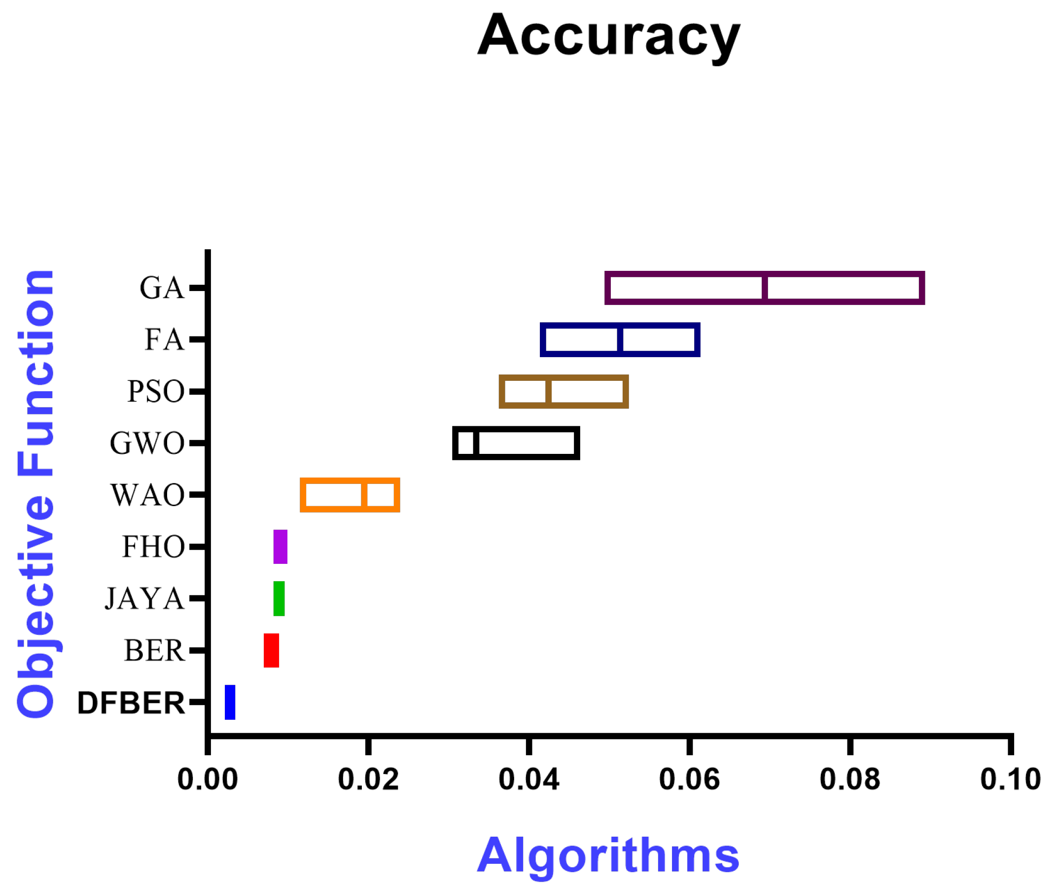
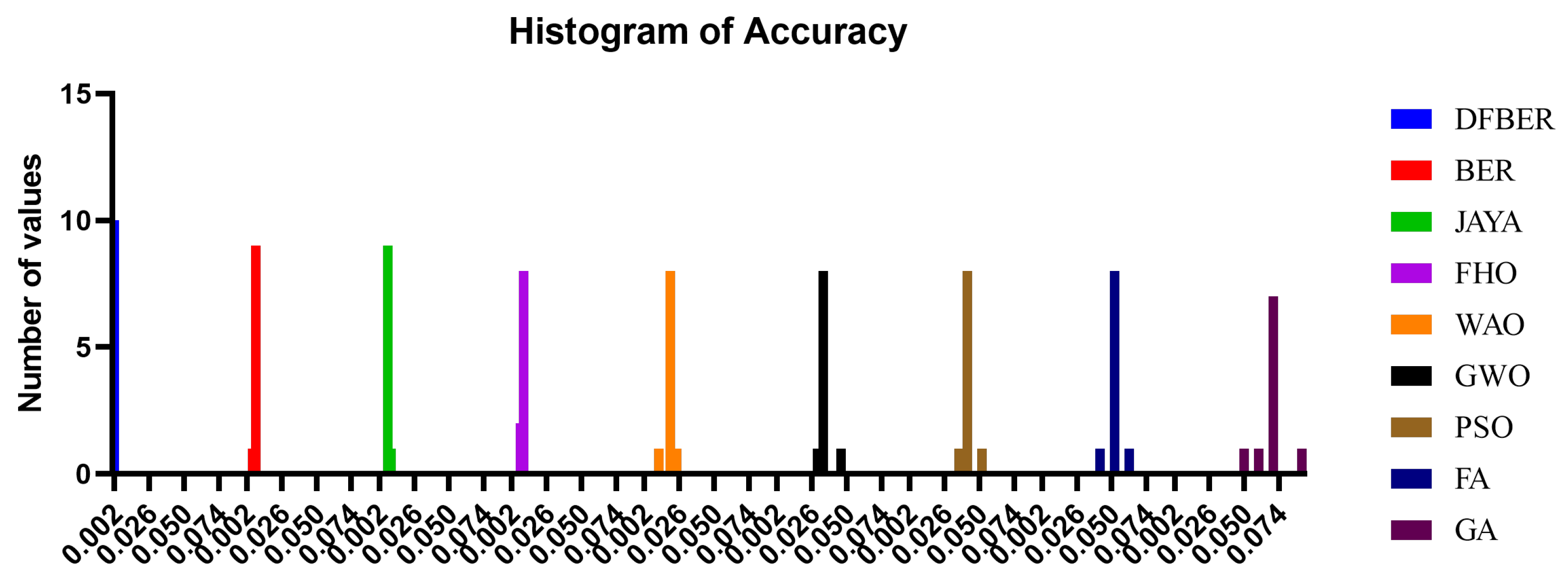
| RNN-DFBER | 0.002843 | 0.000230 | 0.000596 | 0.999325 | 0.999106 | 0.301785 | 0.999106 | 0.998771 |
| RNN-DFBER | RNN-BER | RNN-JAYA | RNN-FHO | RNN-WOA | RNN-GWO | RNN-PSO | RNN-FA | |
|---|---|---|---|---|---|---|---|---|
| Number of values | 10 | 10 | 10 | 10 | 10 | 10 | 10 | 10 |
| Minimum | 0.002643 | 0.006966 | 0.008195 | 0.00815 | 0.01146 | 0.03041 | 0.03624 | 0.04138 |
| Maximum | 0.002943 | 0.008897 | 0.009595 | 0.009498 | 0.02395 | 0.04634 | 0.0524 | 0.06138 |
| Range | 0.0003 | 0.001931 | 0.0014 | 0.001348 | 0.01249 | 0.01593 | 0.01616 | 0.02 |
| Mean | 0.002823 | 0.007959 | 0.00894 | 0.009263 | 0.0191 | 0.0344 | 0.04268 | 0.05138 |
| Std. Deviation | 7.89 × 10⁻⁵ | 0.000455 | 0.000331 | 0.000502 | 0.003035 | 0.004299 | 0.003918 | 0.004714 |
| Std. Error of Mean | 2.49 × 10⁻⁵ | 0.000144 | 0.000105 | 0.000159 | 0.00096 | 0.001359 | 0.001239 | 0.001491 |
| Time(S) | 17.85 | 23.56 | 29.15 | 31.24 | 33.68 | 35.45 | 37.87 | 38.17 |
| SS | DF | MS | F (DFn, DFd) | p Value | |
|---|---|---|---|---|---|
| Treatment (between columns) | 0.04257 | 8 | 0.005321 | F (8, 81) = 290.7 | p < 0.0001 |
| Residual (within columns) | 0.001483 | 81 | 0.0000183 | - | - |
| Total | 0.04405 | 89 | - | - | - |
| DFBER | BER | JAYA | FHO | WOA | GWO | PSO | FA | GA | |
|---|---|---|---|---|---|---|---|---|---|
| Theoretical median | 0 | 0 | 0 | 0 | 0 | 0 | 0 | 0 | 0 |
| Actual median | 0.002843 | 0.007966 | 0.008951 | 0.009498 | 0.01946 | 0.03341 | 0.0424 | 0.05138 | 0.06938 |
| Number of values | 10 | 10 | 10 | 10 | 10 | 10 | 10 | 10 | 10 |
| Wilcoxon Signed Rank Test | |||||||||
| Sum of signed ranks (W) | 55 | 55 | 55 | 55 | 55 | 55 | 55 | 55 | 55 |
| Sum of positive ranks | 55 | 55 | 55 | 55 | 55 | 55 | 55 | 55 | 55 |
| Sum of negative ranks | 0 | 0 | 0 | 0 | 0 | 0 | 0 | 0 | 0 |
| p value (two tailed) | 0.002 | 0.002 | 0.002 | 0.002 | 0.002 | 0.002 | 0.002 | 0.002 | 0.002 |
| Exact or estimate? | Exact | Exact | Exact | Exact | Exact | Exact | Exact | Exact | Exact |
| Significant (alpha = 0.05)? | Yes | Yes | Yes | Yes | Yes | Yes | Yes | Yes | Yes |
| How big is the discrepancy? | |||||||||
| Discrepancy | 0.002843 | 0.007966 | 0.008951 | 0.009498 | 0.01946 | 0.03341 | 0.0424 | 0.05138 | 0.06938 |
Disclaimer/Publisher’s Note: The statements, opinions and data contained in all publications are solely those of the individual author(s) and contributor(s) and not of MDPI and/or the editor(s). MDPI and/or the editor(s) disclaim responsibility for any injury to people or property resulting from any ideas, methods, instructions or products referred to in the content. |
© 2023 by the authors. Licensee MDPI, Basel, Switzerland. This article is an open access article distributed under the terms and conditions of the Creative Commons Attribution (CC BY) license (https://creativecommons.org/licenses/by/4.0/).
Share and Cite
Karim, F.K.; Khafaga, D.S.; Eid, M.M.; Towfek, S.K.; Alkahtani, H.K. A Novel Bio-Inspired Optimization Algorithm Design for Wind Power Engineering Applications Time-Series Forecasting. Biomimetics 2023, 8, 321. https://doi.org/10.3390/biomimetics8030321
Karim FK, Khafaga DS, Eid MM, Towfek SK, Alkahtani HK. A Novel Bio-Inspired Optimization Algorithm Design for Wind Power Engineering Applications Time-Series Forecasting. Biomimetics. 2023; 8(3):321. https://doi.org/10.3390/biomimetics8030321
Chicago/Turabian StyleKarim, Faten Khalid, Doaa Sami Khafaga, Marwa M. Eid, S. K. Towfek, and Hend K. Alkahtani. 2023. "A Novel Bio-Inspired Optimization Algorithm Design for Wind Power Engineering Applications Time-Series Forecasting" Biomimetics 8, no. 3: 321. https://doi.org/10.3390/biomimetics8030321