


Reptile Search Algorithm Considering Different Flight Heights to Solve Engineering Optimization Design Problems
 , ,
, ,
Abstract
:1. Introduction
2. RSA
| Algorithm 1. Pseudo-code of RSA | |
| 1. | Define Dim, UB, LB, Max_Iter(T), Curr_Iter(t), α, β, etc |
| 2. | Initialize the population randomly |
| 3. | while (t < T) do |
| 4. | Evaluate the fitness of each |
| 5. | Find Best solution |
| 6. | Update the ES using Equation (6). |
| 7. | for (i = 1 to m) do |
| 8. | for (j = 1 to n) do |
| 9. | Update the η, R, P and values using Equations (4), (5) and (7), respectively. |
| 10. | If (t ≤ T/4) then |
| 11. | Calculate using Equation (3) |
| 12. | else if (t ≤ 2T/4 and t > T/4) then |
| 13. | Calculate using Equation (3) |
| 14. | else if (t ≤ 3T/4 and t > 2T/4) then |
| 15. | Calculate using Equation (8) |
| 16. | else |
| 17. | Calculate using Equation (8) |
| 19. | end if |
| 20. | end for |
| 21. | end for |
| 22. | t = t+1 |
| 23. | end while |
| 24. | Return the best solution. |
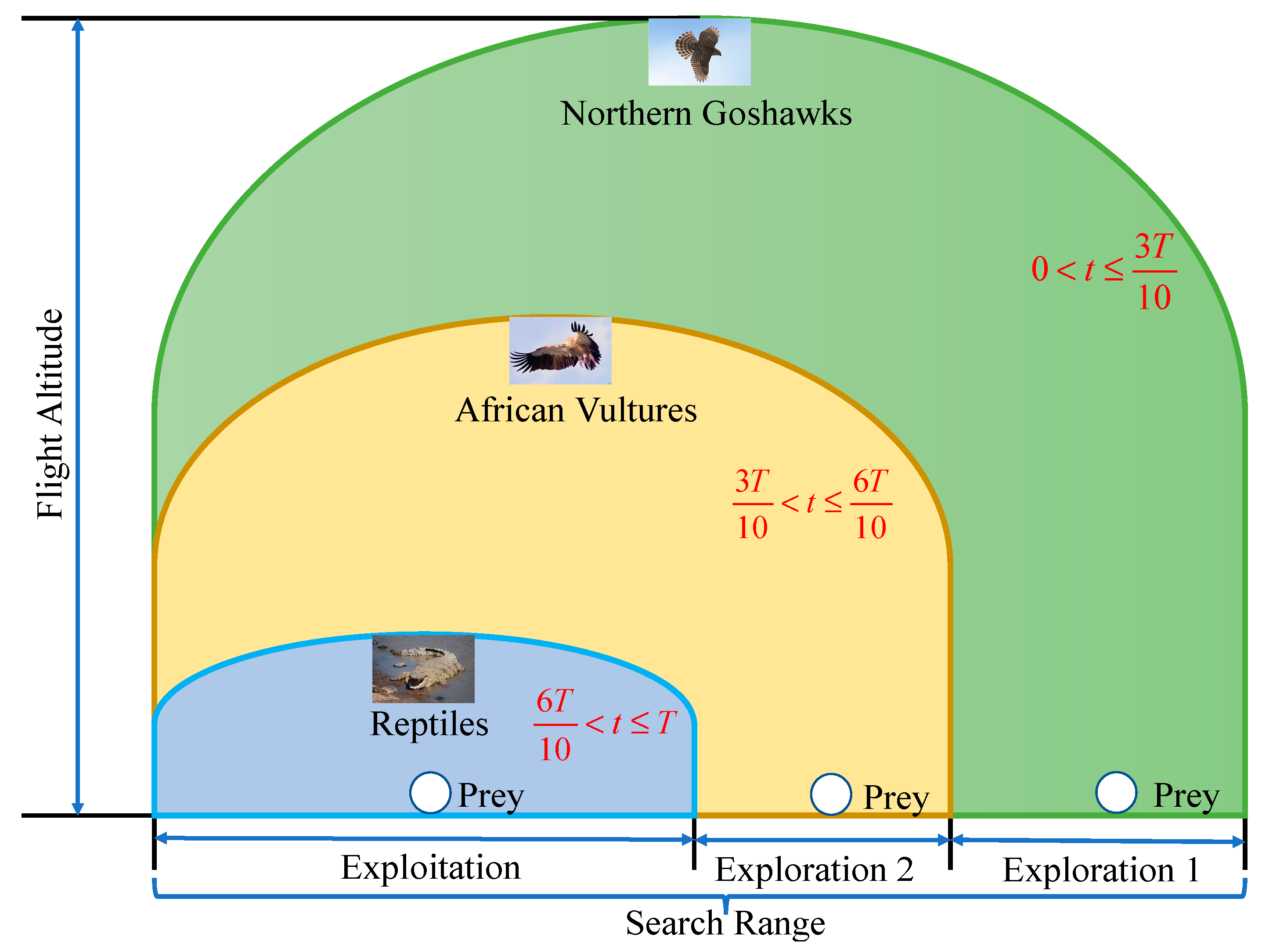
3. Proposed FRSA
3.1. High-Altitude Search Mechanism (Northern Goshawk Exploration)
3.2. Low-Altitude Search Mechanism (African Vulture Exploration)
3.3. Novel Dynamic Factor
| Algorithm 2. Pseudo-code of FRSA | |
| 1. | Define Dim, UB, LB, Max_Iter(T), Curr_Iter(t), α, β, etc |
| 2. | Initialize the population randomly |
| 3. | while (t < T) do |
| 4. | Evaluate the fitness of each |
| 5. | Find Best solution |
| 6. | Update the ES using Equation (6). |
| 7. | for (i = 1 to m) do |
| 8. | for (j = 1 to n) do |
| 9. | Update the η, R, P and values using Equations (4), (5) and (7), respectively. |
| 10. | if (t ≤ 3T/10) then |
| 11. | Calculate using Equation (10) |
| 12. | else if (t ≤ 6T/10 and t > 3T/10) then |
| 13. | Calculate using Equation (14) |
| 14. | else if (t ≤ 8T/10 and t > 6T/10) then |
| 15. | Calculate using Equation (15) |
| 16. | else |
| 17. | Calculate using Equation (15) |
| 18. | end if |
| 19. | end for |
| 20. | end for |
| 21. | t = t + 1 |
| 22. | end while |
| 23. | Return best solution. |
3.4. Computational Time Complexity of the FRSA
4. Analysis of Experiments and Results
4.1. Benchmark Function Sets and Compared Algorithms
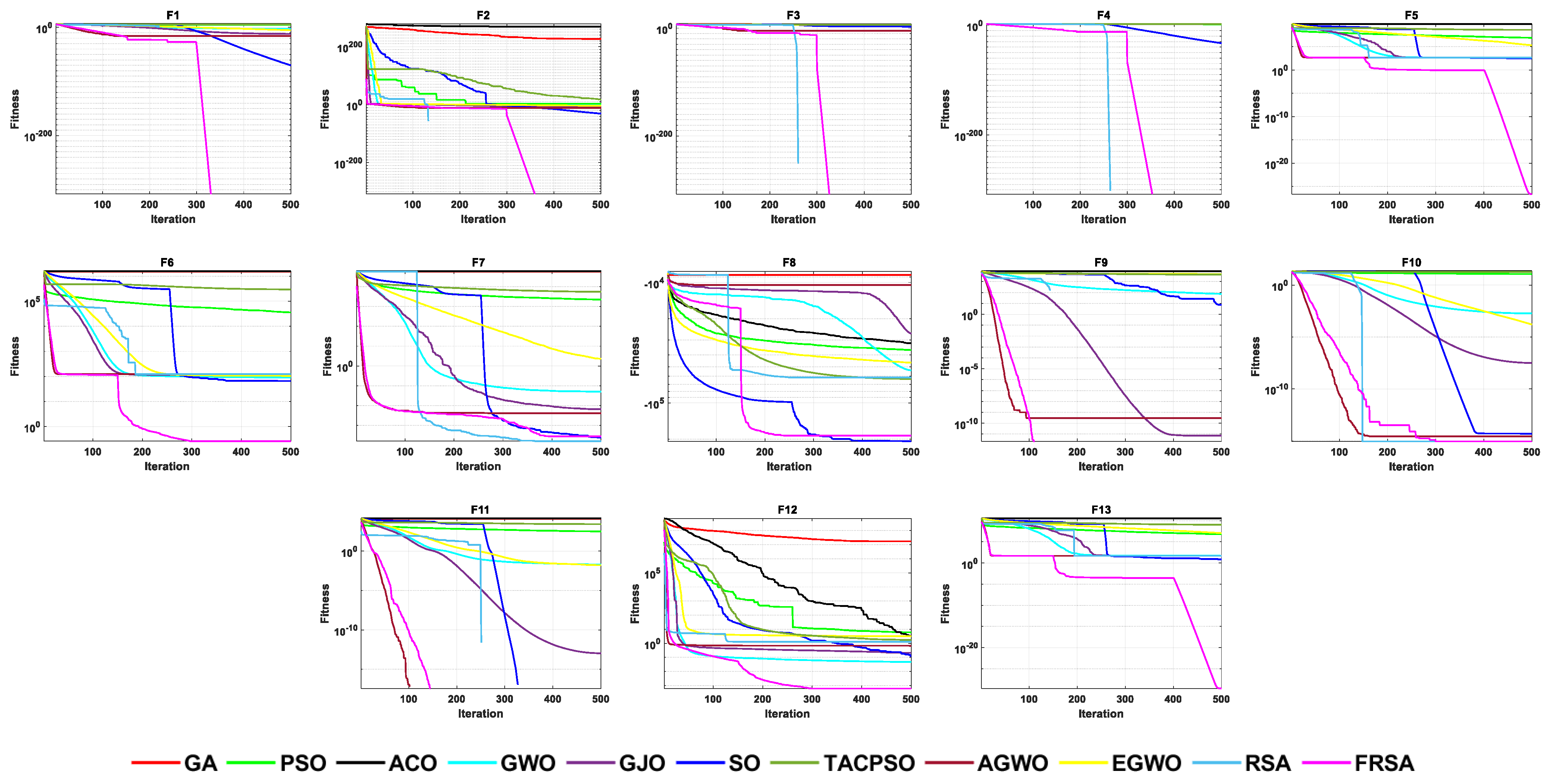
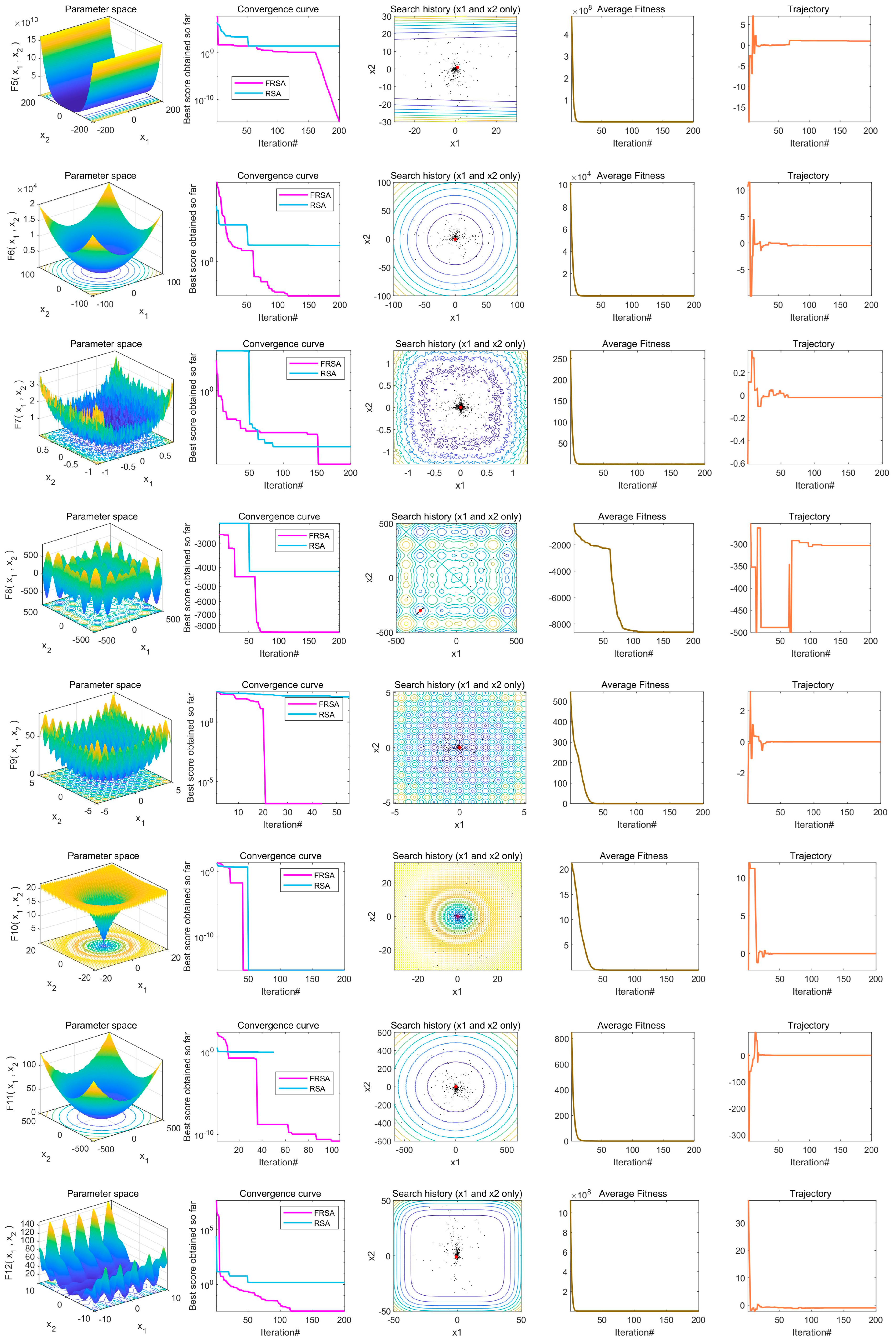
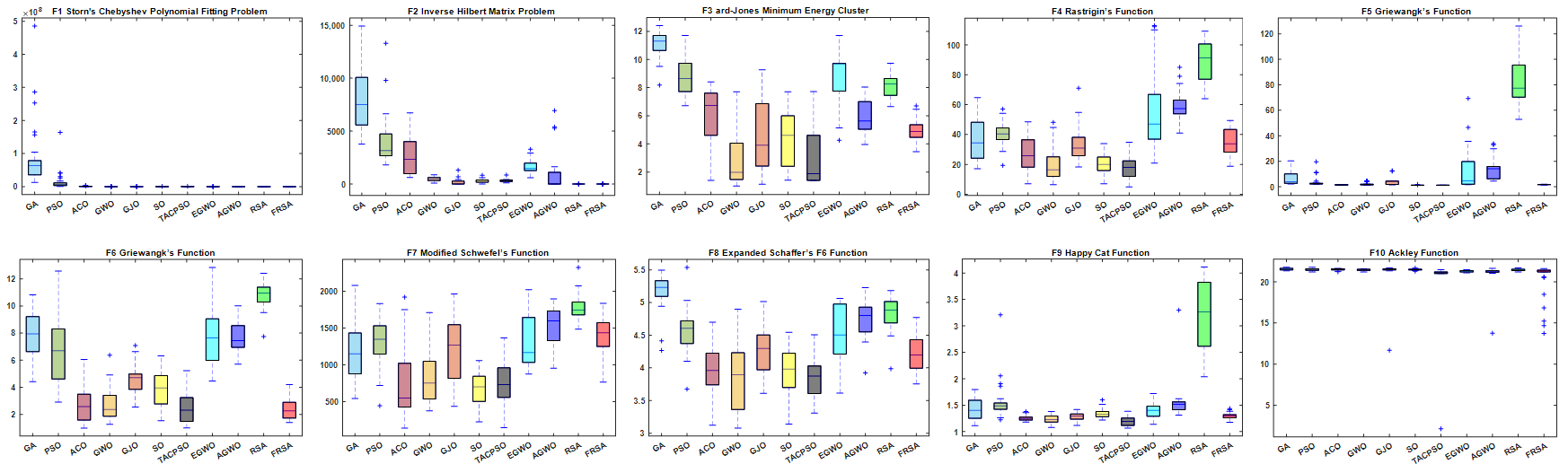
4.2. Results Comparison and Analysis
5. Real-World Engineering Design Problems
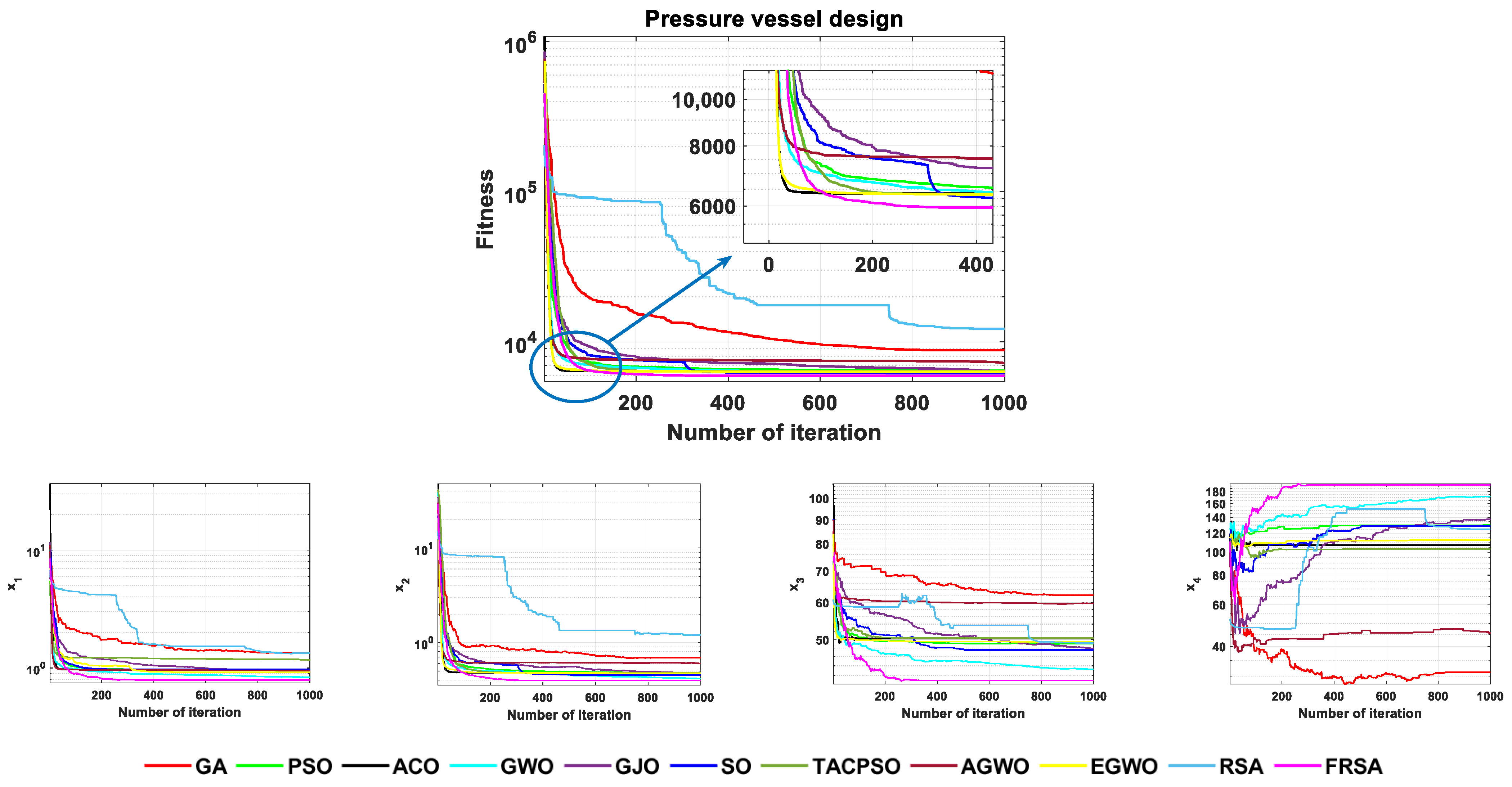
5.1. Pressure Vessel Design
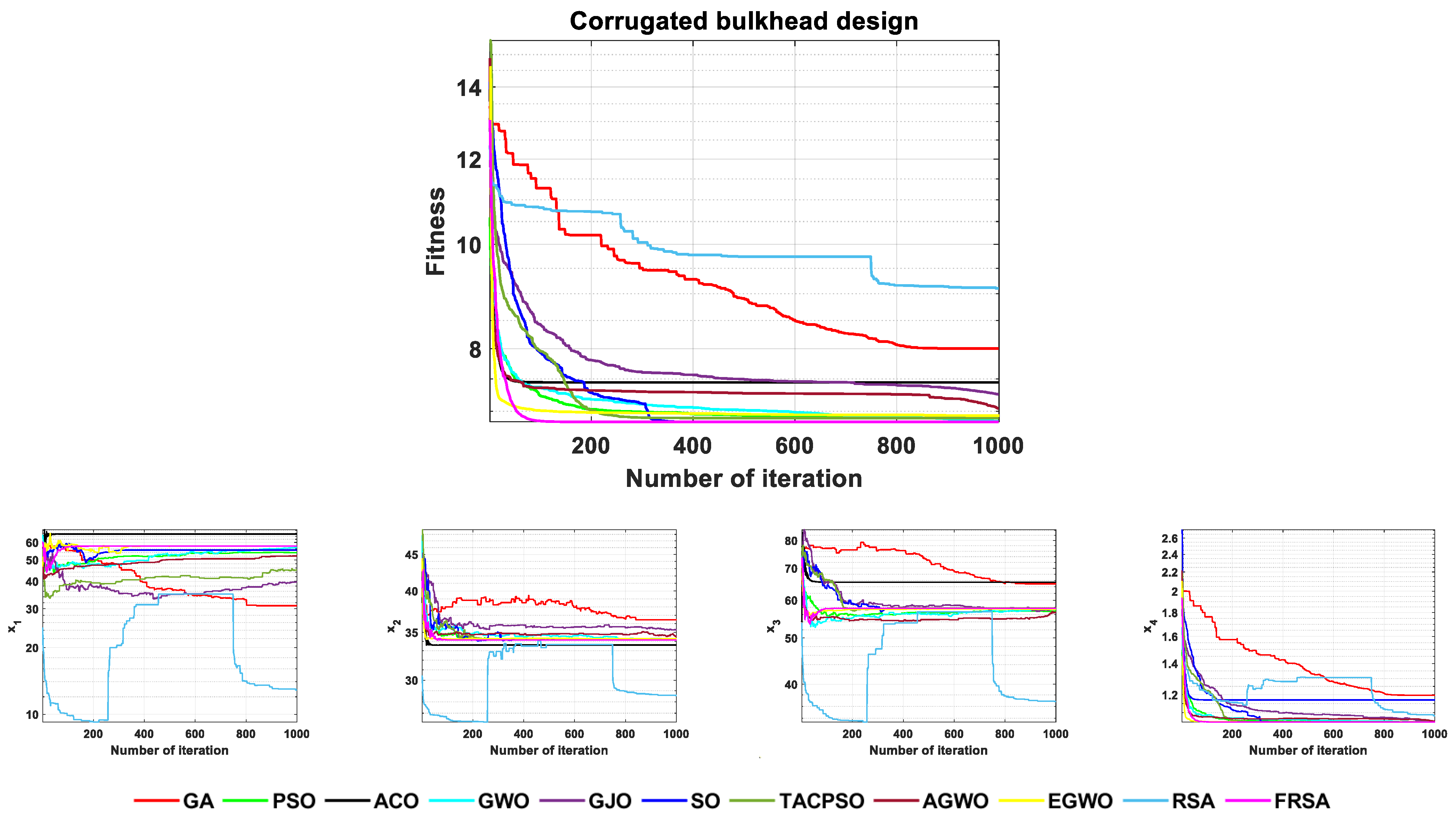
5.2. Corrugated Bulkhead Design
5.3. Welded Beam Design
6. Conclusions and Future Work
Author Contributions
Funding
Institutional Review Board Statement
Informed Consent Statement
Data Availability Statement
Conflicts of Interest
References
- Barkhoda, W.; Sheikhi, H. Immigrant imperialist competitive algorithm to solve the multi-constraint node placement problem in target-based wireless sensor networks. Ad Hoc Netw. 2020, 106, 102183. [Google Scholar] [CrossRef]
- Fu, Z.; Wu, Y.; Liu, X. A tensor-based deep LSTM forecasting model capturing the intrinsic connection in multivariate time series. Appl. Intell. 2022, 53, 15873–15888. [Google Scholar] [CrossRef]
- Liao, C.; Shi, K.; Zhao, X. Predicting the extreme loads in power production of large wind turbines using an improved PSO algorithm. Appl. Sci. 2019, 9, 521. [Google Scholar] [CrossRef] [Green Version]
- Wei, J.; Huang, H.; Yao, L.; Hu, Y.; Fan, Q.; Huang, D. New imbalanced bearing fault diagnosis method based on Sample-characteristic Oversampling TechniquE (SCOTE) and multi-class LS-SVM. Appl. Soft Comput. 2021, 101, 107043. [Google Scholar] [CrossRef]
- Shi, J.; Zhang, G.; Sha, J. Jointly pricing and ordering for a multi-product multi-constraint newsvendor problem with supplier quantity discounts. Appl. Math. Model. 2011, 35, 3001–3011. [Google Scholar] [CrossRef]
- Wu, Y.; Fu, Z.; Liu, X.; Bing, Y. A hybrid stock market prediction model based on GNG and reinforcement learning. Expert Syst. Appl. 2023, 228, 120474. [Google Scholar] [CrossRef]
- Sadollah, A.; Choi, Y.; Kim, J.H. Metaheuristic optimization algorithms for approximate solutions to ordinary differential equations. In Proceedings of the 2015 IEEE Congress on Evolutionary Computation (CEC), Sendai, Japan, 25–28 May 2015; pp. 792–798. [Google Scholar]
- Mahdavi, S.; Shiri, M.E.; Rahnamayan, S. Metaheuristics in large-scale global continues optimization: A survey. Inf. Sci. 2015, 295, 407–428. [Google Scholar] [CrossRef]
- Yang, X.-S. Nature-inspired optimization algorithms: Challenges and open problems. J. Comput. Sci. 2020, 46, 101104. [Google Scholar] [CrossRef] [Green Version]
- Heidari, A.A.; Mirjalili, S.; Faris, H.; Aljarah, I.; Mafarja, M.; Chen, H. Harris hawks optimization: Algorithm and applications. Future Gener. Comput. Syst. 2019, 97, 849–872. [Google Scholar] [CrossRef]
- Mirjalili, S.; Gandomi, A.H.; Mirjalili, S.Z.; Saremi, S.; Faris, H.; Mirjalili, S.M. Salp Swarm Algorithm: A bio-inspired optimizer for engineering design problems. Adv. Eng. Softw. 2017, 114, 163–191. [Google Scholar] [CrossRef]
- Chou, J.-S.; Nguyen, N.-M. FBI inspired meta-optimization. Appl. Soft Comput. 2020, 93, 106339. [Google Scholar] [CrossRef]
- Askari, Q.; Younas, I.; Saeed, M. Political Optimizer: A novel socio-inspired meta-heuristic for global optimization. Knowl.-Based Syst. 2020, 195, 105709. [Google Scholar] [CrossRef]
- Hatamlou, A. Black hole: A new heuristic optimization approach for data clustering. Inf. Sci. 2013, 222, 175–184. [Google Scholar] [CrossRef]
- Abedinpourshotorban, H.; Mariyam Shamsuddin, S.; Beheshti, Z.; Jawawi, D.N.A. Electromagnetic field optimization: A physics-inspired metaheuristic optimization algorithm. Swarm Evol. Comput. 2016, 26, 8–22. [Google Scholar] [CrossRef]
- Holland, J.H. Genetic algorithms. Sci. Am. 1992, 267, 66–73. [Google Scholar] [CrossRef]
- Kennedy, J.; Eberhart, R. Particle swarm optimization. In Proceedings of the IEEE ICNN’95-International Conference on Neural Networks, Perth, WA, Australia, 27 November–1 December 1995; pp. 1942–1948. [Google Scholar]
- Dorigo, M.; Birattari, M.; Stutzle, T. Ant colony optimization. IEEE Comput. Intell. Mag. 2006, 1, 28–39. [Google Scholar] [CrossRef]
- Mirjalili, S.; Mirjalili, S.M.; Lewis, A. Grey wolf optimizer. Adv. Eng. Softw. 2014, 69, 46–61. [Google Scholar] [CrossRef] [Green Version]
- Wolpert, D.H.; Macready, W.G. No free lunch theorems for optimization. IEEE Trans. Evol. Comput. 1997, 1, 67–82. [Google Scholar] [CrossRef] [Green Version]
- Fan, Q.; Huang, H.; Li, Y.; Han, Z.; Hu, Y.; Huang, D. Beetle antenna strategy based grey wolf optimization. Expert Syst. Appl. 2021, 165, 113882. [Google Scholar] [CrossRef]
- Ma, C.; Huang, H.; Fan, Q.; Wei, J.; Du, Y.; Gao, W. Grey wolf optimizer based on Aquila exploration method. Expert Syst. Appl. 2022, 205, 117629. [Google Scholar] [CrossRef]
- Yuan, P.; Zhang, T.; Yao, L.; Lu, Y.; Zhuang, W. A Hybrid Golden Jackal Optimization and Golden Sine Algorithm with Dynamic Lens-Imaging Learning for Global Optimization Problems. Appl. Sci. 2022, 12, 9709. [Google Scholar] [CrossRef]
- Yao, L.; Yuan, P.; Tsai, C.-Y.; Zhang, T.; Lu, Y.; Ding, S. ESO: An enhanced snake optimizer for real-world engineering problems. Expert Syst. Appl. 2023, 230, 120594. [Google Scholar] [CrossRef]
- Abualigah, L.; Elaziz, M.A.; Sumari, P.; Geem, Z.W.; Gandomi, A.H. Reptile Search Algorithm (RSA): A nature-inspired meta-heuristic optimizer. Expert Syst. Appl. 2022, 191, 116158. [Google Scholar] [CrossRef]
- Ervural, B.; Hakli, H. A binary reptile search algorithm based on transfer functions with a new stochastic repair method for 0–1 knapsack problems. Comput. Ind. Eng. 2023, 178, 109080. [Google Scholar] [CrossRef]
- Emam, M.M.; Houssein, E.H.; Ghoniem, R.M. A modified reptile search algorithm for global optimization and image segmentation: Case study brain MRI images. Comput. Biol. Med. 2023, 152, 106404. [Google Scholar] [CrossRef] [PubMed]
- Xiong, J.; Peng, T.; Tao, Z.; Zhang, C.; Song, S.; Nazir, M.S. A dual-scale deep learning model based on ELM-BiLSTM and improved reptile search algorithm for wind power prediction. Energy 2023, 266, 126419. [Google Scholar] [CrossRef]
- Elkholy, M.; Elymany, M.; Yona, A.; Senjyu, T.; Takahashi, H.; Lotfy, M.E. Experimental validation of an AI-embedded FPGA-based Real-Time smart energy management system using Multi-Objective Reptile search algorithm and gorilla troops optimizer. Energy Convers. 2023, 282, 116860. [Google Scholar] [CrossRef]
- Abdollahzadeh, B.; Gharehchopogh, F.S.; Mirjalili, S. African vultures optimization algorithm: A new nature-inspired metaheuristic algorithm for global optimization problems. Comput. Ind. Eng. 2021, 158, 107408. [Google Scholar] [CrossRef]
- Dehghani, M.; Hubálovský, Š.; Trojovský, P. Northern goshawk optimization: A new swarm-based algorithm for solving optimization problems. IEEE Access 2021, 9, 162059–162080. [Google Scholar] [CrossRef]
- Bansal, S. Performance comparison of five metaheuristic nature-inspired algorithms to find near-OGRs for WDM systems. Artif. Intell. Rev. 2020, 53, 5589–5635. [Google Scholar] [CrossRef]
- Chopra, N.; Ansari, M.M. Golden jackal optimization: A novel nature-inspired optimizer for engineering applications. Expert Syst. Appl. 2022, 198, 116924. [Google Scholar] [CrossRef]
- Hashim, F.A.; Hussien, A.G. Snake Optimizer: A novel meta-heuristic optimization algorithm. Knowl.-Based Syst. 2022, 242, 108320. [Google Scholar] [CrossRef]
- Ziyu, T.; Dingxue, Z. A modified particle swarm optimization with an adaptive acceleration coefficients. In Proceedings of the 2009 Asia-Pacific Conference on Information Processing, Shenzhen, China, 18–19 July 2009; pp. 330–332. [Google Scholar]
- Komathi, C.; Umamaheswari, M. Design of gray wolf optimizer algorithm-based fractional order PI controller for power factor correction in SMPS applications. IEEE Trans. Power Electron. 2019, 35, 2100–2118. [Google Scholar] [CrossRef]
- Fan, Q.; Huang, H.; Chen, Q.; Yao, L.; Yang, K.; Huang, D. A modified self-adaptive marine predators algorithm: Framework and engineering applications. Eng. Comput. 2021, 38, 3269–3294. [Google Scholar] [CrossRef]
- Abualigah, L.; Almotairi, K.H.; Al-qaness, M.A.A.; Ewees, A.A.; Yousri, D.; Elaziz, M.A.; Nadimi-Shahraki, M.H. Efficient text document clustering approach using multi-search Arithmetic Optimization Algorithm. Knowl.-Based Syst. 2022, 248, 108833. [Google Scholar] [CrossRef]
- Rosner, B.; Glynn, R.J.; Ting Lee, M.L. Incorporation of clustering effects for the Wilcoxon rank sum test: A large-sample approach. Biometrics 2003, 59, 1089–1098. [Google Scholar] [CrossRef]
- Yang, X.-S.; Huyck, C.R.; Karamanoğlu, M.; Khan, N. True global optimality of the pressure vessel design problem: A benchmark for bio-inspired optimisation algorithms. Int. J. Bio-Inspired Comput. 2014, 5, 329–335. [Google Scholar] [CrossRef]
- Braik, M.S. Chameleon Swarm Algorithm: A bio-inspired optimizer for solving engineering design problems. Expert Syst. Appl. 2021, 174, 114685. [Google Scholar] [CrossRef]
- Ravindran, A.R.; Ragsdell, K.M.; Reklaitis, G.V. Engineering Optimization: Methods and Applications; Wiley: Hoboken, NJ, USA, 1983. [Google Scholar]
- Bayzidi, H.; Talatahari, S.; Saraee, M.; Lamarche, C.-P. Social Network Search for Solving Engineering Optimization Problems. Comput. Intell. Neurosci. 2021, 2021, 8548639. [Google Scholar] [CrossRef]
- Coello Coello, C.A. Use of a self-adaptive penalty approach for engineering optimization problems. Comput. Ind. 2000, 41, 113–127. [Google Scholar] [CrossRef]


| Function | Dim | Range | Type | |
|---|---|---|---|---|
| 30,100,500 | [−100, 100] | 0 | Unimodal | |
| 30,100,500 | [−1.28, 1.28] | 0 | Unimodal | |
| 30,100,500 | [−100, 100] | 0 | Unimodal | |
| 30,100,500 | [−100, 100] | 0 | Unimodal | |
| 30,100,500 | [−30, 30] | 0 | Unimodal | |
| 30,100,500 | [−100, 100] | 0 | Unimodal | |
| 30,100,500 | [−1.28, 1.28] | 0 | Unimodal | |
| 30,100,500 | [−500, 500] | −418.9829 × n | Multimodal | |
| 30,100,500 | [−5.12, 5.12] | 0 | Multimodal | |
| 30,100,500 | [−32, 32] | 0 | Multimodal | |
| 30,100,500 | [−600, 600] | 0 | Multimodal | |
| 30,100,500 | [−50, 50] | 0 | Multimodal | |
| 30,100,500 | [−50, 50] | 0 | Multimodal | |
| 2 | [−65.536, 65.536] | 1 | Multimodal | |
| 4 | [−5, 5] | 0.0003 | Multimodal | |
| 2 | [−5, 5] | −1.0316 | Multimodal | |
| 2 | [−5, 5] | 0.398 | Multimodal | |
| 2 | [−2, 2] | 3 | Multimodal | |
| 3 | [0, 1] | −3.86 | Multimodal | |
| 6 | [0, 1] | −3.32 | Multimodal | |
| 4 | [0, 10] | −10.1532 | Multimodal | |
| 4 | [0, 10] | −10.4029 | Multimodal | |
| 4 | [0, 10] | −10.5364 | Multimodal |
| No. | Functions | Dim | Range | |
|---|---|---|---|---|
| F1 | Storn’s Chebyshev Polynomial Fitting Problem | 9 | [−8192, 8192] | 1 |
| F2 | Inverse Hilbert Matrix Problem | 16 | [−16,384, 16,384] | 1 |
| F3 | Lennard–Jones Minimum Energy Cluster | 18 | [−4, 4] | 1 |
| F4 | Rastrigin’s Function | 10 | [−100, 100] | 1 |
| F5 | Griewangk’s Function | 10 | [−100, 100] | 1 |
| F6 | Weierstrass Function | 10 | [−100, 100] | 1 |
| F7 | Modified Schwefel’s Function | 10 | [−100, 100] | 1 |
| F8 | Expanded Schaffer’s F6 Function | 10 | [−100, 100] | 1 |
| F9 | Happy Cat Function | 10 | [−100, 100] | 1 |
| F10 | Ackley Function | 10 | [−100, 100] | 1 |
| Algorithms | Parameters and Assignments |
|---|---|
| GA | |
| PSO | , , , |
| ACO | |
| GWO | , , |
| GJO | |
| SO | |
| TACPSO | , , , |
| AGWO | , |
| EGWO | , , |
| RSA | |
| FRSA |
| F(x) | GA | PSO | ACO | GWO | GJO | SO | TACPSO | AGWO | EGWO | RSA | FRSA | |
|---|---|---|---|---|---|---|---|---|---|---|---|---|
| F1 | Mean | 2.0706 × 10⁴ | 3.3853 × 10² | 4.5737 × 10⁻³ | 1.0329 × 10⁻²⁷ | 1.7311 × 10−54 | 3.9891 × 10−94 | 1.5111 × 10⁻¹ | 3.2767 × 10−317 | 1.2009 × 10⁻³⁰ | 0.0000 × 100 | 0.0000 × 100 |
| Std | 7.1489 × 10³ | 1.6168 × 10² | 6.7589 × 10⁻³ | 1.0808 × 10⁻²⁷ | 4.1785 × 10−54 | 1.0339 × 10−93 | 2.3348 × 10⁻¹ | 0.0000 × 100 | 3.8756 × 10⁻³⁰ | 0.0000 × 100 | 0.0000 × 100 | |
| F2 | Mean | 5.6471 × 101 | 1.7592 × 101 | 2.5207 × 10⁻³ | 1.0724 × 10⁻¹⁶ | 2.0077 × 10⁻³² | 1.8981 × 10−42 | 1.5195 × 100 | 6.1333 × 10−175 | 8.6619 × 10⁻²⁰ | 0.0000 × 100 | 0.0000 × 100 |
| Std | 9.9694 × 100 | 9.9392 × 100 | 1.9247 × 10⁻³ | 8.1353 × 10⁻¹⁷ | 2.6567 × 10⁻³² | 7.8124 × 10−42 | 3.0452 × 100 | 0.0000 × 100 | 2.0027 × 10⁻¹⁹ | 0.0000 × 100 | 0.0000 × 100 | |
| F3 | Mean | 5.2325 × 10⁴ | 8.7587 × 10³ | 3.2509 × 10⁴ | 1.0617 × 10⁻⁵ | 8.0928 × 10⁻¹⁸ | 8.5384 × 10−56 | 1.1348 × 10³ | 5.2178 × 10−264 | 1.2199 × 10⁻³ | 0.0000 × 100 | 0.0000 × 100 |
| Std | 1.5868 × 10⁴ | 5.3330 × 10³ | 7.1037 × 10³ | 2.7063 × 10⁻⁵ | 2.6301 × 10⁻¹⁷ | 3.6611 × 10−55 | 1.1917 × 10³ | 0.0000 × 100 | 4.0506 × 10⁻³ | 0.0000 × 100 | 0.0000 × 100 | |
| F4 | Mean | 7.0290 × 101 | 1.0057 × 101 | 8.3925 × 101 | 7.6327 × 10⁻⁷ | 5.5119 × 10⁻¹⁶ | 5.6706 × 10−40 | 9.7094 × 100 | 8.5240 × 10−155 | 3.5666 × 10⁻¹ | 0.0000 × 100 | 0.0000 × 100 |
| Std | 7.2884 × 100 | 2.6342 × 100 | 1.1652 × 101 | 8.4243 × 10⁻⁷ | 1.3025 × 10⁻¹⁵ | 1.9765 × 10−39 | 3.4154 × 100 | 4.3706 × 10−154 | 1.3297 × 100 | 0.0000 × 100 | 0.0000 × 100 | |
| F5 | Mean | 2.1143 × 10⁷ | 1.3458 × 10⁴ | 6.3852 × 10² | 2.6950 × 101 | 2.7744 × 101 | 2.0242 × 101 | 4.2784 × 10² | 2.8334 × 101 | 2.7928 × 101 | 1.7547 × 101 | 9.0588 × 10⁻²⁹ |
| Std | 1.5073 × 10⁷ | 9.7957 × 10³ | 9.3899 × 10² | 7.1489 × 10⁻¹ | 7.5092 × 10⁻¹ | 1.1160 × 101 | 9.0541 × 10² | 3.9161 × 10⁻¹ | 8.8237 × 10⁻¹ | 1.4272 × 101 | 1.3586 × 10⁻²⁹ | |
| F6 | Mean | 2.2120 × 10⁴ | 3.3844 × 10² | 2.8991 × 10⁻³ | 6.9336 × 10⁻¹ | 2.5998 × 100 | 7.4686 × 10⁻¹ | 2.8608 × 10⁻¹ | 5.1108 × 100 | 3.1744 × 100 | 6.9887 × 100 | 9.3967 × 10⁻³ |
| Std | 8.1756 × 10³ | 1.3189 × 10² | 4.3952 × 10⁻³ | 3.2769 × 10⁻¹ | 4.5246 × 10⁻¹ | 7.2966 × 10⁻¹ | 7.1367 × 10⁻¹ | 3.2531 × 10⁻¹ | 6.9967 × 10⁻¹ | 4.0996 × 10⁻¹ | 7.3219 × 10⁻³ | |
| F7 | Mean | 1.4246 × 101 | 1.4084 × 100 | 9.2893 × 10⁻² | 2.1075 × 10⁻³ | 5.1434 × 10⁻⁴ | 2.9363 × 10⁻⁴ | 8.4275 × 10⁻² | 1.2253 × 10⁻⁴ | 7.9773 × 10⁻³ | 1.2720 × 10⁻⁴ | 3.2019 × 10⁻⁴ |
| Std | 6.4862 × 100 | 5.8085 × 100 | 3.6308 × 10⁻² | 1.4913 × 10⁻³ | 3.3543 × 10⁻⁴ | 2.2856 × 10⁻⁴ | 3.3336 × 10⁻² | 9.7020 × 10⁻⁵ | 4.0919 × 10⁻³ | 1.4087 × 10⁻⁴ | 3.1313 × 10⁻⁴ | |
| F8 | Mean | −2.1820 × 10³ | −8.0517 × 10³ | −7.2210 × 10³ | −5.8586 × 10³ | −4.3233 × 10³ | −1.248 × 10⁴ | −8.6030 × 10³ | −2.7317 × 10³ | −6.5965 × 10³ | −5.4035 × 10³ | −1.1553 × 10⁴ |
| Std | 4.0040 × 10² | 9.6639 × 10² | 1.0003 × 10³ | 7.5792 × 10² | 1.2048 × 10³ | 2.3899 × 10² | 4.6512 × 10² | 4.6201 × 10² | 7.6715 × 10² | 3.1866 × 10² | 1.6853 × 10³ | |
| F9 | Mean | 2.5863 × 10² | 2.0098 × 10² | 2.4292 × 10² | 1.8876 × 100 | 0.0000 × 100 | 5.2470 × 100 | 7.3533 × 101 | 0.0000 × 100 | 1.5967 × 10² | 0.0000 × 100 | 0.0000 × 100 |
| Std | 4.5208 × 101 | 2.1856 × 101 | 2.2226 × 101 | 2.5924 × 100 | 0.0000 × 100 | 1.2881 × 101 | 1.8901 × 101 | 0.0000 × 100 | 3.8336 × 101 | 0.0000 × 100 | 0.0000 × 100 | |
| F10 | Mean | 1.9867 × 101 | 5.3154 × 100 | 1.2859 × 101 | 1.0297 × 10⁻¹³ | 7.2831 × 10⁻¹⁵ | 2.8853 × 10⁻¹ | 2.2423 × 100 | 1.7171 × 10⁻¹⁵ | 1.9107 × 10⁻¹ | 8.8818 × 10⁻¹⁶ | 8.8818 × 10⁻¹⁶ |
| Std | 4.6960 × 10⁻¹ | 1.0010 × 100 | 9.8810 × 100 | 1.8565 × 10⁻¹⁴ | 1.4454 × 10⁻¹⁵ | 7.5143 × 10⁻¹ | 7.3942 × 10⁻¹ | 1.5283 × 10⁻¹⁵ | 7.3243 × 10⁻¹ | 0.0000 × 100 | 0.0000 × 100 | |
| F11 | Mean | 1.8735 × 10² | 4.0848 × 100 | 1.7211 × 10⁻¹ | 4.9998 × 10⁻³ | 0.0000 × 100 | 9.1944 × 10⁻² | 1.3227 × 10⁻¹ | 0.0000 × 100 | 1.1550 × 10⁻² | 0.0000 × 100 | 0.0000 × 100 |
| Std | 6.6774 × 101 | 1.8224 × 100 | 2.7165 × 10⁻¹ | 8.7540 × 10⁻³ | 0.0000 × 100 | 1.7896 × 10⁻¹ | 1.5411 × 10⁻¹ | 0.0000 × 100 | 2.1161 × 10⁻² | 0.0000 × 100 | 0.0000 × 100 | |
| F12 | Mean | 1.7475 × 10⁷ | 5.9962 × 100 | 3.2016 × 100 | 4.7372 × 10⁻² | 2.1168 × 10⁻¹ | 1.2141 × 10⁻¹ | 1.7178 × 100 | 6.7014 × 10⁻¹ | 3.1555 × 100 | 1.2588 × 100 | 6.1299 × 10⁻⁴ |
| Std | 2.4583 × 10⁷ | 3.0819 × 100 | 5.8093 × 100 | 3.6729 × 10⁻² | 6.8287 × 10⁻² | 2.4035 × 10⁻¹ | 1.6616 × 100 | 1.4300 × 10⁻¹ | 3.1014 × 100 | 3.4982 × 10⁻¹ | 4.8674 × 10⁻⁴ | |
| F13 | Mean | 5.7420 × 10⁷ | 2.8474 × 101 | 2.2313 × 100 | 6.8191 × 10⁻¹ | 1.7212 × 100 | 4.8266 × 10⁻¹ | 4.1897 × 100 | 2.5629 × 100 | 2.6787 × 100 | 4.1579 × 10⁻¹ | 3.8688 × 10⁻³¹ |
| Std | 4.5158 × 10⁷ | 2.9526 × 101 | 5.0535 × 100 | 2.5619 × 10⁻¹ | 2.4044 × 10⁻¹ | 6.9409 × 10⁻¹ | 4.8206 × 100 | 8.7892 × 10⁻² | 5.8772 × 10⁻¹ | 8.3308 × 10⁻¹ | 2.0585 × 10⁻³¹ | |
| Friedman value | 1.0423 × 101 | 9.2692 × 100 | 8.3846 × 100 | 5.1538 × 100 | 4.6923 × 100 | 4.7308 × 100 | 7.5385 × 100 | 3.5385 × 100 | 6.8077 × 100 | 3.2500 × 100 | 2.2115 × 100 | |
| Friedman rank | 11 | 10 | 9 | 6 | 4 | 5 | 8 | 3 | 7 | 2 | 1 | |
| F(x) | GA | PSO | ACO | GWO | GJO | SO | TACPSO | AGWO | EGWO | RSA | FRSA | |
|---|---|---|---|---|---|---|---|---|---|---|---|---|
| F1 | Mean | 2.2803 × 10⁵ | 4.8382 × 10³ | 1.1718 × 10⁵ | 1.2883 × 10⁻¹² | 7.5690 × 10⁻²⁸ | 7.3577 × 10−82 | 6.3258 × 10³ | 2.3337 × 10−244 | 2.9059 × 10⁻¹⁶ | 0.0000 × 100 | 0.0000 × 100 |
| Std | 2.6407 × 10⁴ | 2.6614 × 10³ | 1.2634 × 10⁴ | 7.2714 × 10⁻¹³ | 2.0721 × 10⁻²⁷ | 1.6214 × 10−81 | 1.9044 × 10³ | 0.0000 × 100 | 4.3702 × 10⁻¹⁶ | 0.0000 × 100 | 0.0000 × 100 | |
| F2 | Mean | 1.3878 × 10³ | 7.9551 × 101 | 1.0183 × 1024 | 4.0761 × 10⁻⁸ | 1.7716 × 10⁻¹⁷ | 1.1687 × 10⁻³⁵ | 1.0765 × 10² | 3.5171 × 10−127 | 2.1585 × 10⁻¹⁰ | 0.0000 × 100 | 0.0000 × 100 |
| Std | 6.1674 × 10³ | 2.0688 × 101 | 4.2616 × 1024 | 1.2357 × 10⁻⁸ | 1.9050 × 10⁻¹⁷ | 1.1341 × 10⁻³⁵ | 2.4822 × 101 | 1.9264 × 10−126 | 2.7251 × 10⁻¹⁰ | 0.0000 × 100 | 0.0000 × 100 | |
| F3 | Mean | 6.4151 × 10⁵ | 1.2058 × 10⁵ | 5.4194 × 10⁵ | 5.4654 × 10² | 1.1960 × 100 | 1.9856 × 10⁻²⁷ | 7.9658 × 10⁴ | 9.4366 × 10−220 | 2.3095 × 10⁴ | 0.0000 × 100 | 0.0000 × 100 |
| Std | 1.8635 × 10⁵ | 7.0068 × 10⁴ | 5.8785 × 10⁴ | 5.7433 × 10² | 5.0520 × 100 | 1.0876 × 10⁻²⁶ | 1.7856 × 10⁴ | 0.0000 × 100 | 1.5626 × 10⁴ | 0.0000 × 100 | 0.0000 × 100 | |
| F4 | Mean | 9.4654 × 101 | 2.1438 × 101 | 9.7253 × 101 | 1.3792 × 100 | 5.4031 × 100 | 1.1115 × 10−36 | 4.4837 × 101 | 1.4570 × 10−130 | 7.1629 × 101 | 0.0000 × 100 | 0.0000 × 100 |
| Std | 1.8813 × 100 | 4.9340 × 100 | 1.1638 × 100 | 1.5201 × 100 | 8.6012 × 100 | 1.6885 × 10−36 | 3.1827 × 100 | 5.4253 × 10−130 | 8.6435 × 100 | 0.0000 × 100 | 0.0000 × 100 | |
| F5 | Mean | 8.5046 × 10⁸ | 5.2446 × 10⁵ | 1.0445 × 10⁹ | 9.7690 × 101 | 9.8283 × 101 | 6.4281 × 101 | 3.2768 × 10⁶ | 9.8749 × 101 | 9.8175 × 101 | 9.8988 × 101 | 3.8975 × 10⁻²⁸ |
| Std | 1.4410 × 10⁸ | 4.6652 × 10⁵ | 2.9092 × 10⁸ | 7.8639 × 10⁻¹ | 4.8343 × 10⁻¹ | 4.1497 × 101 | 2.0490 × 10⁶ | 2.4079 × 10⁻¹ | 6.4582 × 10⁻¹ | 3.7169 × 10⁻³ | 2.2620 × 10⁻²⁹ | |
| F6 | Mean | 2.1753 × 10⁵ | 3.9481 × 10³ | 1.1119 × 10⁵ | 1.0013 × 101 | 1.6765 × 101 | 1.4058 × 101 | 6.3639 × 10³ | 2.2476 × 101 | 1.4930 × 101 | 2.4607 × 101 | 4.1033 × 10⁻² |
| Std | 2.1653 × 10⁴ | 1.5048 × 10³ | 1.1425 × 10⁴ | 1.2537 × 100 | 7.1104 × 10⁻¹ | 1.0657 × 101 | 2.8579 × 10³ | 3.1181 × 10⁻¹ | 1.0606 × 100 | 2.0760 × 10⁻¹ | 2.9663 × 10⁻² | |
| F7 | Mean | 1.2316 × 10³ | 5.3044 × 101 | 8.4073 × 10² | 7.4525 × 10⁻³ | 1.2061 × 10⁻³ | 2.2315 × 10⁻⁴ | 8.4554 × 100 | 2.5098 × 10⁻⁴ | 2.9401 × 10⁻² | 1.1850 × 10⁻⁴ | 2.4755 × 10⁻⁴ |
| Std | 2.2446 × 10² | 8.5484 × 101 | 3.3353 × 10² | 2.8388 × 10⁻³ | 5.1273 × 10⁻⁴ | 2.4369 × 10⁻⁴ | 4.9534 × 100 | 2.3744 × 10⁻⁴ | 1.2773 × 10⁻² | 9.1632 × 10⁻⁵ | 2.2133 × 10⁻⁴ | |
| F8 | Mean | −4.1683 × 10³ | −1.5010 × 10⁴ | −1.5812 × 10⁴ | −1.6026 × 10⁴ | −9.1616 × 10³ | −4.1583 × 10⁴ | −2.2513 × 10⁴ | −5.0509 × 10³ | −1.7702 × 10⁴ | −1.7056 × 10⁴ | −3.6466 × 10⁴ |
| Std | 9.7178 × 10² | 2.6230 × 10³ | 2.7296 × 10³ | 2.4537 × 10³ | 4.2288 × 10³ | 5.2761 × 10² | 1.9590 × 10³ | 9.0114 × 10² | 1.4842 × 10³ | 7.6478 × 10² | 7.1490 × 10³ | |
| F9 | Mean | 1.5280 × 10³ | 8.7473 × 10² | 1.3949 × 10³ | 1.0982 × 101 | 1.5158 × 10⁻¹⁴ | 1.4159 × 101 | 4.6367 × 10² | 0.0000 × 100 | 8.3312 × 10² | 0.0000 × 100 | 0.0000 × 100 |
| Std | 6.4386 × 101 | 8.6547 × 101 | 4.5366 × 101 | 8.3224 × 100 | 5.7687 × 10⁻¹⁴ | 3.0090 × 101 | 5.1780 × 101 | 0.0000 × 100 | 1.4958 × 10² | 0.0000 × 100 | 0.0000 × 100 | |
| F10 | Mean | 2.0786 × 101 | 9.0803 × 100 | 2.0778 × 101 | 1.1377 × 10⁻⁷ | 5.0271 × 10⁻¹⁴ | 4.4409 × 10⁻¹⁵ | 1.2679 × 101 | 4.2040 × 10⁻¹⁵ | 8.4006 × 10⁻² | 8.8818 × 10⁻¹⁶ | 8.8818 × 10⁻¹⁶ |
| Std | 1.0176 × 10⁻¹ | 2.4931 × 100 | 4.0391 × 10⁻² | 3.5782 × 10⁻⁸ | 9.8451 × 10⁻¹⁵ | 0.0000 × 100 | 1.0867 × 100 | 9.0135 × 10⁻¹⁶ | 4.6012 × 10⁻¹ | 0.0000 × 100 | 0.0000 × 100 | |
| F11 | Mean | 1.9914 × 10³ | 3.5916 × 101 | 1.0510 × 10³ | 5.6641 × 10⁻³ | 0.0000 × 100 | 0.0000 × 100 | 5.5387 × 101 | 0.0000 × 100 | 5.0051 × 10⁻³ | 0.0000 × 100 | 0.0000 × 100 |
| Std | 2.1758 × 10² | 1.3366 × 101 | 1.1905 × 10² | 1.2302 × 10⁻² | 0.0000 × 100 | 0.0000 × 100 | 1.6313 × 101 | 0.0000 × 100 | 8.8528 × 10⁻³ | 0.0000 × 100 | 0.0000 × 100 | |
| F12 | Mean | 1.7624 × 10⁹ | 2.4562 × 10³ | 3.1606 × 10⁹ | 2.5960 × 10⁻¹ | 6.0942 × 10⁻¹ | 1.7964 × 10⁻¹ | 1.4874 × 10⁵ | 1.0179 × 100 | 1.0922 × 101 | 1.2477 × 100 | 2.3383 × 10⁻⁴ |
| Std | 4.3233 × 10⁸ | 1.3099 × 10⁴ | 3.0994 × 10⁸ | 5.0711 × 10⁻² | 7.7430 × 10⁻² | 3.7770 × 10⁻¹ | 4.4671 × 10⁵ | 6.5885 × 10⁻² | 8.0541 × 100 | 8.0783 × 10⁻² | 2.0208 × 10⁻⁴ | |
| F13 | Mean | 3.4134 × 10⁹ | 4.4552 × 10⁴ | 5.6359 × 10⁹ | 6.8948 × 100 | 8.3742 × 100 | 2.1756 × 100 | 2.4624 × 10⁶ | 9.6505 × 100 | 2.6571 × 101 | 9.6741 × 100 | 6.2822 × 10⁻³¹ |
| Std | 6.5988 × 10⁸ | 8.5336 × 10⁴ | 5.0013 × 10⁸ | 4.6552 × 10⁻¹ | 2.3595 × 10⁻¹ | 3.7113 × 100 | 2.2076 × 10⁶ | 6.1528 × 10⁻² | 3.9839 × 101 | 5.8643 × 10⁻¹ | 1.8088 × 10⁻³¹ | |
| Friedman value | 1.0077 × 101 | 8.4615 × 100 | 9.6923 × 100 | 5.4231 × 100 | 5.0769 × 100 | 3.8077 × 100 | 8.3077 × 100 | 3.5385 × 100 | 6.6923 × 100 | 2.9038 × 100 | 2.0192 × 100 | |
| Friedman rank | 11 | 9 | 10 | 6 | 5 | 4 | 8 | 3 | 7 | 2 | 1 | |
| F(x) | GA | PSO | ACO | GWO | GJO | SO | TACPSO | AGWO | EGWO | RSA | FRSA | |
|---|---|---|---|---|---|---|---|---|---|---|---|---|
| F1 | Mean | 1.5128 × 10⁶ | 3.9219 × 10⁴ | 1.5590 × 10⁶ | 1.8644 × 10⁻³ | 9.6545 × 10⁻¹³ | 7.1375 × 10−71 | 2.9775 × 10⁵ | 1.9542 × 10⁻¹⁶ | 6.1307 × 10⁻⁶ | 0.0000 × 100 | 0.0000 × 100 |
| Std | 3.6434 × 10⁴ | 1.3201 × 10⁴ | 3.6597 × 10⁴ | 7.6449 × 10⁻⁴ | 9.7800 × 10⁻¹³ | 2.4182 × 10−70 | 1.9178 × 10⁴ | 1.0703 × 10⁻¹⁵ | 6.2289 × 10⁻⁶ | 0.0000 × 100 | 0.0000 × 100 | |
| F2 | Mean | 6.0554 × 10226 | 4.5845 × 10² | 4.1585 × 10268 | 1.0881 × 10⁻² | 6.4312 × 10⁻⁹ | 1.2654 × 10⁻³¹ | 6.3084 × 10¹⁷ | 9.6613 × 10⁻¹² | 1.8407 × 10⁻⁴ | 0.0000 × 100 | 0.0000 × 100 |
| Std | Inf | 1.2379 × 10² | Inf | 1.7840 × 10⁻³ | 4.2103 × 10⁻⁹ | 1.7875 × 10⁻³¹ | 3.4548 × 10¹⁸ | 5.2623 × 10⁻¹¹ | 1.4881 × 10⁻⁴ | 0.0000 × 100 | 0.0000 × 100 | |
| F3 | Mean | 2.1316 × 10⁷ | 2.8293 × 10⁶ | 1.3418 × 10⁷ | 3.1425 × 10⁵ | 5.1301 × 10⁴ | 8.2145 × 10² | 2.0650 × 10⁶ | 1.2415 × 10⁻⁵ | 1.5987 × 10⁶ | 0.0000 × 100 | 0.0000 × 100 |
| Std | 6.9901 × 10⁶ | 1.4370 × 10⁶ | 1.3908 × 10⁶ | 7.7943 × 10⁴ | 5.3267 × 10⁴ | 4.4993 × 10³ | 4.4012 × 10⁵ | 4.9557 × 10⁻⁵ | 2.9634 × 10⁵ | 0.0000 × 100 | 0.0000 × 100 | |
| F4 | Mean | 9.9161 × 101 | 3.5159 × 101 | 9.9451 × 101 | 6.5006 × 101 | 8.2792 × 101 | 1.4350 × 10⁻³³ | 7.0229 × 101 | 9.2608 × 101 | 9.6997 × 101 | 0.0000 × 100 | 0.0000 × 100 |
| Std | 2.3489 × 10⁻¹ | 5.2254 × 100 | 1.9881 × 10⁻¹ | 4.1463 × 100 | 4.3209 × 100 | 1.9441 × 10⁻³³ | 2.9160 × 100 | 2.5175 × 101 | 9.6498 × 10⁻¹ | 0.0000 × 100 | 0.0000 × 100 | |
| F5 | Mean | 6.7974 × 10⁹ | 8.5251 × 10⁶ | 7.3446 × 10⁹ | 4.9803 × 10² | 4.9826 × 10² | 3.3551 × 10² | 4.1692 × 10⁸ | 4.9892 × 10² | 2.0683 × 10⁵ | 4.9899 × 10² | 2.3167 × 10⁻²⁷ |
| Std | 2.6217 × 10⁸ | 5.6668 × 10⁶ | 3.3600 × 10⁸ | 3.5404 × 10⁻¹ | 1.4870 × 10⁻¹ | 2.1069 × 10² | 3.9772 × 10⁷ | 6.8551 × 10⁻² | 3.5928 × 10⁵ | 6.2629 × 10⁻³ | 6.3915 × 10⁻²⁹ | |
| F6 | Mean | 1.5114 × 10⁶ | 3.5914 × 10⁴ | 1.5648 × 10⁶ | 9.1100 × 101 | 1.1002 × 10² | 6.6077 × 101 | 2.9553 × 10⁵ | 1.2326 × 10² | 1.0553 × 10² | 1.2463 × 10² | 2.6280 × 10⁻¹ |
| Std | 3.8311 × 10⁴ | 1.7013 × 10⁴ | 3.9734 × 10⁴ | 1.8331 × 100 | 1.2181 × 100 | 5.6041 × 101 | 1.6752 × 10⁴ | 4.2145 × 10⁻¹ | 1.6851 × 100 | 2.1010 × 10⁻¹ | 2.2051 × 10⁻¹ | |
| F7 | Mean | 5.6877 × 10⁴ | 2.2092 × 10³ | 5.9688 × 10⁴ | 5.1280 × 10⁻² | 6.5673 × 10⁻³ | 2.4772 × 10⁻⁴ | 5.5137 × 10³ | 4.1447 × 10⁻³ | 2.2992 × 100 | 1.6209 × 10⁻⁴ | 2.8637 × 10⁻⁴ |
| Std | 1.7801 × 10³ | 1.1383 × 10³ | 2.5418 × 10³ | 1.2074 × 10⁻² | 3.9213 × 10⁻³ | 1.6724 × 10⁻⁴ | 1.0697 × 10³ | 2.4388 × 10⁻³ | 2.0536 × 100 | 1.9236 × 10⁻⁴ | 2.5568 × 10⁻⁴ | |
| F8 | Mean | −8.6802 × 10³ | −3.6383 × 10⁴ | −3.1971 × 10⁴ | −5.3591 × 10⁴ | −2.6579 × 10⁴ | −2.0786 × 10⁵ | −6.3227 × 10⁴ | −1.0502 × 10⁴ | −4.6206 × 10⁴ | −6.1323 × 10⁴ | −1.8676 × 10⁵ |
| Std | 1.6314 × 10³ | 5.2307 × 10³ | 6.0899 × 10³ | 1.3793 × 10⁴ | 1.4002 × 10⁴ | 3.1591 × 10³ | 2.8055 × 10³ | 1.2858 × 10³ | 2.9204 × 10³ | 5.3327 × 10³ | 3.2489 × 10⁴ | |
| F9 | Mean | 8.6929 × 10³ | 4.4339 × 10³ | 8.8775 × 10³ | 7.5607 × 101 | 7.3063 × 10⁻¹² | 7.3183 × 100 | 4.4337 × 10³ | 3.0028 × 10⁻¹⁰ | 5.0232 × 10³ | 0.0000 × 100 | 0.0000 × 100 |
| Std | 1.2985 × 10² | 5.4177 × 10² | 1.0714 × 10² | 2.1468 × 101 | 2.8809 × 10⁻¹² | 3.9910 × 101 | 1.3537 × 10² | 1.6447 × 10⁻⁹ | 1.1423 × 10³ | 0.0000 × 100 | 0.0000 × 100 | |
| F10 | Mean | 2.1105 × 101 | 1.1398 × 101 | 2.1018 × 101 | 1.8561 × 10⁻³ | 3.1785 × 10⁻⁸ | 4.9146 × 10⁻¹⁵ | 1.8242 × 101 | 2.6645 × 10⁻¹⁵ | 1.5959 × 10⁻⁴ | 8.8818 × 10⁻¹⁶ | 8.8818 × 10⁻¹⁶ |
| Std | 2.8935 × 10⁻² | 3.5690 × 100 | 1.0087 × 10⁻² | 3.7330 × 10⁻⁴ | 1.5956 × 10⁻⁸ | 1.2283 × 10⁻¹⁵ | 1.9259 × 10⁻¹ | 1.8067 × 10⁻¹⁵ | 9.5884 × 10⁻⁵ | 0.0000 × 100 | 0.0000 × 100 | |
| F11 | Mean | 1.3426 × 10⁴ | 3.0914 × 10² | 1.4057 × 10⁴ | 2.0278 × 10⁻² | 1.0707 × 10⁻¹³ | 0.0000 × 100 | 2.6951 × 10³ | 0.0000 × 100 | 1.6181 × 10⁻² | 0.0000 × 100 | 0.0000 × 100 |
| Std | 3.5235 × 10² | 9.0526 × 101 | 3.4112 × 10² | 4.1331 × 10⁻² | 9.3215 × 10⁻¹⁴ | 0.0000 × 100 | 1.5936 × 10² | 0.0000 × 100 | 3.4848 × 10⁻² | 0.0000 × 100 | 0.0000 × 100 | |
| F12 | Mean | 1.7068 × 10¹⁰ | 2.0914 × 10⁵ | 1.8490 × 10¹⁰ | 7.6115 × 10⁻¹ | 9.3858 × 10⁻¹ | 5.1918 × 10⁻² | 3.4826 × 10⁸ | 1.1681 × 100 | 5.9375 × 10⁷ | 1.2016 × 100 | 2.1631 × 10⁻⁴ |
| Std | 7.0596 × 10⁸ | 3.1495 × 10⁵ | 6.2478 × 10⁸ | 7.5436 × 10⁻² | 2.6207 × 10⁻² | 2.0980 × 10⁻¹ | 7.1676 × 10⁷ | 1.0173 × 10⁻² | 6.2911 × 10⁷ | 2.9273 × 10⁻³ | 2.1681 × 10⁻⁴ | |
| F13 | Mean | 3.1399 × 10¹⁰ | 6.4059 × 10⁶ | 3.3112 × 10¹⁰ | 5.0441 × 101 | 4.7911 × 101 | 7.2088 × 100 | 1.1450 × 10⁹ | 4.9797 × 101 | 1.1536 × 10⁷ | 4.9921 × 101 | 2.0996 × 10⁻³⁰ |
| Std | 1.3772 × 10⁹ | 8.1295 × 10⁶ | 1.3777 × 10⁹ | 1.4970 × 100 | 3.2400 × 10⁻¹ | 1.4763 × 101 | 1.5104 × 10⁸ | 4.1931 × 10⁻² | 1.7631 × 10⁷ | 3.9674 × 10⁻² | 9.4926 × 10⁻³² | |
| Friedman value | 9.6346 × 100 | 8.0385 × 100 | 9.9808 × 100 | 5.9231 × 100 | 5.1154 × 100 | 3.5000 × 100 | 8.1538 × 100 | 4.3077 × 100 | 6.7692 × 100 | 2.6154 × 100 | 1.9615 × 100 | |
| Friedman rank | 10 | 8 | 11 | 6 | 5 | 3 | 9 | 4 | 7 | 2 | 1 | |
| F(x) | GA | PSO | ACO | GWO | GJO | SO | TACPSO | AGWO | EGWO | RSA | FRSA | |
|---|---|---|---|---|---|---|---|---|---|---|---|---|
| F14 | Mean | 1.1036 × 100 | 9.9800 × 10⁻¹ | 2.8537 × 100 | 5.0796 × 100 | 5.3036 × 100 | 1.0022 × 100 | 1.0311 × 100 | 6.4801 × 100 | 7.7381 × 100 | 4.1376 × 100 | 9.9823 × 10⁻¹ |
| Std | 3.3201 × 10⁻¹ | 2.1481 × 10⁻¹⁰ | 3.8575 × 100 | 4.1695 × 100 | 4.4384 × 100 | 2.0981 × 10⁻² | 1.8148 × 10⁻¹ | 4.3221 × 100 | 4.4611 × 100 | 3.1646 × 100 | 1.2224 × 10⁻³ | |
| F15 | Mean | 1.3902 × 10⁻² | 1.0272 × 10⁻² | 5.3931 × 10⁻³ | 3.0739 × 10⁻³ | 8.5798 × 10⁻⁴ | 6.0445 × 10⁻⁴ | 5.2544 × 10⁻⁴ | 1.4132 × 10⁻³ | 1.0979 × 10⁻² | 1.7245 × 10⁻³ | 4.1525 × 10⁻⁴ |
| Std | 1.0043 × 10⁻² | 1.0209 × 10⁻² | 8.4021 × 10⁻³ | 6.8994 × 10⁻³ | 2.0507 × 10⁻³ | 3.3346 × 10⁻⁴ | 4.1271 × 10⁻⁴ | 2.7639 × 10⁻³ | 2.3937 × 10⁻² | 1.4282 × 10⁻³ | 8.1372 × 10⁻⁵ | |
| F16 | Mean | −9.4538 × 10⁻¹ | −1.0316 × 100 | −1.0316 × 100 | −1.0316 × 100 | −1.0316 × 100 | −1.0316 × 100 | −1.0316 × 100 | −1.0306 × 100 | −1.0316 × 100 | −1.0305 × 100 | −1.0316 × 100 |
| Std | 1.1796 × 10⁻¹ | 1.5212 × 10⁻⁵ | 6.7752 × 10⁻¹⁶ | 1.8976 × 10⁻⁸ | 2.5177 × 10⁻⁷ | 5.2964 × 10⁻¹⁶ | 5.9036 × 10⁻¹⁶ | 5.7742 × 10⁻³ | 5.6187 × 10⁻⁹ | 1.4232 × 10⁻³ | 1.8373 × 10⁻¹³ | |
| F17 | Mean | 4.0005 × 10⁻¹ | 3.9789 × 10⁻¹ | 3.9789 × 10⁻¹ | 3.9789 × 10⁻¹ | 3.9789 × 10⁻¹ | 3.9789 × 10⁻¹ | 3.9789 × 10⁻¹ | 3.9794 × 10⁻¹ | 3.9789 × 10⁻¹ | 4.1970 × 10⁻¹ | 3.9789 × 10⁻¹ |
| Std | 4.0846 × 10⁻³ | 1.4541 × 10⁻⁵ | 0.0000 × 100 | 7.2876 × 10⁻⁷ | 9.0667 × 10⁻⁶ | 0.0000 × 100 | 0.0000 × 100 | 5.3183 × 10⁻⁵ | 5.9598 × 10⁻⁷ | 2.4368 × 10⁻² | 0.0000 × 100 | |
| F18 | Mean | 1.0596 × 101 | 3.0002 × 100 | 3.0000 × 100 | 3.0000 × 100 | 3.0000 × 100 | 3.0000 × 100 | 3.0000 × 100 | 3.0000 × 100 | 3.9001 × 100 | 4.0014 × 100 | 3.0000 × 100 |
| Std | 1.1443 × 101 | 2.8621 × 10⁻⁴ | 6.6995 × 10⁻¹⁶ | 4.8544 × 10⁻⁵ | 8.5395 × 10⁻⁶ | 2.7088 × 10⁻¹⁵ | 2.1599 × 10⁻¹⁵ | 1.8450 × 10⁻⁶ | 4.9295 × 100 | 5.4822 × 100 | 3.7510 × 10⁻¹⁵ | |
| F19 | Mean | −3.2754 × 100 | −3.8614 × 100 | −3.8628 × 100 | −3.8612 × 100 | −3.8581 × 100 | −3.8370 × 100 | −3.8628 × 100 | −3.8569 × 100 | −3.8618 × 100 | −3.7992 × 100 | −3.8628 × 100 |
| Std | 3.2324 × 10⁻¹ | 2.9771 × 10⁻³ | 2.7101 × 10⁻¹⁵ | 2.6343 × 10⁻³ | 3.7740 × 10⁻³ | 1.4113 × 10⁻¹ | 2.6117 × 10⁻¹⁵ | 2.6408 × 10⁻³ | 2.6029 × 10⁻³ | 6.3061 × 10⁻² | 2.0748 × 10⁻¹⁵ | |
| F20 | Mean | −1.4764 × 100 | −3.0759 × 100 | −3.2467 × 100 | −3.2796 × 100 | −3.0914 × 100 | −3.2982 × 100 | −3.2665 × 100 | −3.1263 × 100 | −3.2177 × 100 | −2.7566 × 100 | −3.3213 × 100 |
| Std | 4.8085 × 10⁻¹ | 1.9536 × 10⁻¹ | 5.8273 × 10⁻² | 6.9288 × 10⁻² | 1.3582 × 10⁻¹ | 4.8370 × 10⁻² | 6.0328 × 10⁻² | 1.0519 × 10⁻¹ | 9.9155 × 10⁻² | 3.4506 × 10⁻¹ | 2.7018 × 10⁻³ | |
| F21 | Mean | −8.5022 × 10⁻¹ | −9.0585 × 100 | −5.9936 × 100 | −9.0574 × 100 | −7.7219 × 100 | −1.0138 × 101 | −6.8143 × 100 | −7.3462 × 100 | −6.2985 × 100 | −5.0552 × 100 | −1.0105 × 101 |
| Std | 5.1246 × 10⁻¹ | 2.0337 × 100 | 3.7255 × 100 | 2.2621 × 100 | 2.9320 × 100 | 3.4059 × 10⁻² | 3.4941 × 100 | 2.9488 × 100 | 3.1346 × 100 | 3.1204 × 10⁻⁷ | 7.9343 × 10⁻² | |
| F22 | Mean | −1.0336 × 100 | −9.0891 × 100 | −7.4926 × 100 | −1.0401 × 101 | −9.8499 × 100 | −1.0290 × 101 | −7.1316 × 100 | −8.5041 × 100 | −7.1293 × 100 | −5.0877 × 100 | −1.0402 × 101 |
| Std | 4.4156 × 10⁻¹ | 2.6893 × 100 | 3.6556 × 100 | 1.2043 × 10⁻³ | 1.6359 × 100 | 2.5749 × 10⁻¹ | 3.4330 × 100 | 2.5694 × 100 | 3.6624 × 100 | 8.0616 × 10⁻⁷ | 4.1384 × 10⁻³ | |
| F23 | Mean | −1.2002 × 100 | −9.0372 × 100 | −7.2815 × 100 | −9.9938 × 100 | −9.6040 × 100 | −1.0469 × 101 | −9.4877 × 100 | −8.6658 × 100 | −6.4546 × 100 | −5.1314 × 100 | −1.0525 × 101 |
| Std | 3.9772 × 10⁻¹ | 2.6192 × 100 | 3.8049 × 100 | 2.0583 × 100 | 2.4090 × 100 | 1.4991 × 10⁻¹ | 2.4300 × 100 | 2.5916 × 100 | 3.8996 × 100 | 1.6091 × 10⁻² | 3.3992 × 10⁻² | |
| Friedman value | 9.2000 × 100 | 6.4000 × 100 | 5.8250 × 100 | 5.1500 × 100 | 6.2000 × 100 | 3.4250 × 100 | 4.5250 × 100 | 7.3000 × 100 | 7.8500 × 100 | 7.8000 × 100 | 2.3250 × 100 | |
| Friedman rank | 11 | 7 | 5 | 4 | 6 | 2 | 3 | 8 | 10 | 9 | 1 | |
| F(x) | Dim | GA | PSO | ACO | GWO | GJO | SO | TACPSO | AGWO | EGWO | RSA | Total |
|---|---|---|---|---|---|---|---|---|---|---|---|---|
| F1 | 30 | 1.2118 × 10⁻¹² | 1.2118 × 10⁻¹² | 1.2118 × 10⁻¹² | 1.2118 × 10⁻¹² | 1.2118 × 10⁻¹² | 1.2118 × 10⁻¹² | 1.2118 × 10⁻¹² | 1.2118 × 10⁻¹² | 1.2118 × 10⁻¹² | NaN | 9/1/0 |
| 100 | 1.2118 × 10⁻¹² | 1.2118 × 10⁻¹² | 1.2118 × 10⁻¹² | 1.2118 × 10⁻¹² | 1.2118 × 10⁻¹² | 1.2118 × 10⁻¹² | 1.2118 × 10⁻¹² | 1.2118 × 10⁻¹² | 1.9346 × 10⁻¹⁰ | NaN | 9/1/0 | |
| 500 | 1.2118 × 10⁻¹² | 1.2118 × 10⁻¹² | 1.2118 × 10⁻¹² | 1.2118 × 10⁻¹² | 1.2118 × 10⁻¹² | 1.2118 × 10⁻¹² | 1.2118 × 10⁻¹² | 1.2118 × 10⁻¹² | 1.2118 × 10⁻¹² | NaN | 9/1/0 | |
| F2 | 30 | 1.2118 × 10⁻¹² | 1.2118 × 10⁻¹² | 1.2118 × 10⁻¹² | 1.2118 × 10⁻¹² | 1.2118 × 10⁻¹² | 1.2118 × 10⁻¹² | 1.2118 × 10⁻¹² | 1.2118 × 10⁻¹² | 1.2118 × 10⁻¹² | NaN | 9/1/0 |
| 100 | 1.2118 × 10⁻¹² | 1.2118 × 10⁻¹² | 1.2118 × 10⁻¹² | 1.2118 × 10⁻¹² | 1.2118 × 10⁻¹² | 1.2118 × 10⁻¹² | 1.2118 × 10⁻¹² | 1.2118 × 10⁻¹² | 1.2118 × 10⁻¹² | NaN | 9/1/0 | |
| 500 | 1.2118 × 10⁻¹² | 1.2118 × 10⁻¹² | 1.2118 × 10⁻¹² | 1.2118 × 10⁻¹² | 1.2118 × 10⁻¹² | 1.2118 × 10⁻¹² | 1.2118 × 10⁻¹² | 1.2118 × 10⁻¹² | 1.2118 × 10⁻¹² | NaN | 9/1/0 | |
| F3 | 30 | 1.2118 × 10⁻¹² | 1.2118 × 10⁻¹² | 1.2118 × 10⁻¹² | 1.2118 × 10⁻¹² | 1.2118 × 10⁻¹² | 1.2118 × 10⁻¹² | 1.2118 × 10⁻¹² | 1.2118 × 10⁻¹² | 1.2118 × 10⁻¹² | NaN | 9/1/0 |
| 100 | 1.2118 × 10⁻¹² | 1.2118 × 10⁻¹² | 1.2118 × 10⁻¹² | 1.2118 × 10⁻¹² | 1.2118 × 10⁻¹² | 1.2118 × 10⁻¹² | 1.2118 × 10⁻¹² | 1.2118 × 10⁻¹² | 4.5736 × 10⁻¹² | NaN | 9/1/0 | |
| 500 | 1.2118 × 10⁻¹² | 1.2118 × 10⁻¹² | 1.2118 × 10⁻¹² | 1.2118 × 10⁻¹² | 1.2118 × 10⁻¹² | 1.2118 × 10⁻¹² | 1.2118 × 10⁻¹² | 1.2118 × 10⁻¹² | 1.2118 × 10⁻¹² | NaN | 9/1/0 | |
| F4 | 30 | 1.2118 × 10⁻¹² | 1.2118 × 10⁻¹² | 1.2118 × 10⁻¹² | 1.2118 × 10⁻¹² | 1.2118 × 10⁻¹² | 1.2118 × 10⁻¹² | 1.2118 × 10⁻¹² | 1.2118 × 10⁻¹² | 1.2118 × 10⁻¹² | NaN | 9/1/0 |
| 100 | 1.2118 × 10⁻¹² | 1.2118 × 10⁻¹² | 1.2118 × 10⁻¹² | 1.2118 × 10⁻¹² | 1.2118 × 10⁻¹² | 1.2118 × 10⁻¹² | 1.2118 × 10⁻¹² | 1.2118 × 10⁻¹² | 1.2118 × 10⁻¹² | NaN | 9/1/0 | |
| 500 | 1.2118 × 10⁻¹² | 1.2118 × 10⁻¹² | 1.2118 × 10⁻¹² | 1.2118 × 10⁻¹² | 1.2118 × 10⁻¹² | 1.2118 × 10⁻¹² | 1.2118 × 10⁻¹² | 1.2118 × 10⁻¹² | 1.2118 × 10⁻¹² | NaN | 9/1/0 | |
| F5 | 30 | 3.0161 × 10⁻¹¹ | 3.0161 × 10⁻¹¹ | 3.0161 × 10⁻¹¹ | 3.0161 × 10⁻¹¹ | 3.0161 × 10⁻¹¹ | 3.0161 × 10⁻¹¹ | 3.0161 × 10⁻¹¹ | 3.0161 × 10⁻¹¹ | 3.0161 × 10⁻¹¹ | 3.0161 × 10⁻¹¹ | 10/0/0 |
| 100 | 3.0161 × 10⁻¹¹ | 3.0161 × 10⁻¹¹ | 3.0161 × 10⁻¹¹ | 3.0161 × 10⁻¹¹ | 3.0161 × 10⁻¹¹ | 3.0161 × 10⁻¹¹ | 3.0161 × 10⁻¹¹ | 3.0161 × 10⁻¹¹ | 3.0161 × 10⁻¹¹ | 3.0161 × 10⁻¹¹ | 10/0/0 | |
| 500 | 3.0199 × 10⁻¹¹ | 3.0199 × 10⁻¹¹ | 3.0199 × 10⁻¹¹ | 3.0199 × 10⁻¹¹ | 3.0199 × 10⁻¹¹ | 3.0199 × 10⁻¹¹ | 3.0199 × 10⁻¹¹ | 3.0199 × 10⁻¹¹ | 3.0199 × 10⁻¹¹ | 3.0199 × 10⁻¹¹ | 10/0/0 | |
| F6 | 30 | 3.0199 × 10⁻¹¹ | 3.0199 × 10⁻¹¹ | 2.3168 × 10⁻⁶ | 3.0199 × 10⁻¹¹ | 3.0199 × 10⁻¹¹ | 1.0937 × 10⁻¹⁰ | 3.1573 × 10⁻⁵ | 3.0199 × 10⁻¹¹ | 3.0199 × 10⁻¹¹ | 3.0199 × 10⁻¹¹ | 9/0/1 |
| 100 | 3.0161 × 10⁻¹¹ | 3.0161 × 10⁻¹¹ | 3.0161 × 10⁻¹¹ | 3.0161 × 10⁻¹¹ | 3.0161 × 10⁻¹¹ | 8.9934 × 10⁻¹¹ | 3.0161 × 10⁻¹¹ | 3.0161 × 10⁻¹¹ | 3.0161 × 10⁻¹¹ | 3.0161 × 10⁻¹¹ | 10/0/0 | |
| 500 | 3.0199 × 10⁻¹¹ | 3.0199 × 10⁻¹¹ | 3.0199 × 10⁻¹¹ | 3.0199 × 10⁻¹¹ | 3.0199 × 10⁻¹¹ | 4.9752 × 10⁻¹¹ | 3.0199 × 10⁻¹¹ | 3.0199 × 10⁻¹¹ | 3.0199 × 10⁻¹¹ | 3.0199 × 10⁻¹¹ | 10/0/0 | |
| F7 | 30 | 3.0199 × 10⁻¹¹ | 3.0199 × 10⁻¹¹ | 3.0199 × 10⁻¹¹ | 1.2057 × 10⁻¹⁰ | 1.0315 × 10⁻² | 9.8231 × 10⁻¹ | 3.0199 × 10⁻¹¹ | 3.3384 × 10⁻¹¹ | 3.5010 × 10⁻³ | 1.7666 × 10⁻³ | 7/1/2 |
| 100 | 3.0161 × 10⁻¹¹ | 3.0161 × 10⁻¹¹ | 3.0161 × 10⁻¹¹ | 3.0161 × 10⁻¹¹ | 7.3803 × 10⁻¹⁰ | 6.7350 × 10⁻¹ | 3.0199 × 10⁻¹¹ | 3.0199 × 10⁻¹¹ | 7.0617 × 10⁻¹ | 2.4157 × 10⁻² | 7/2/1 | |
| 500 | 3.0199 × 10⁻¹¹ | 3.0199 × 10⁻¹¹ | 3.0199 × 10⁻¹¹ | 3.0199 × 10⁻¹¹ | 3.0199 × 10⁻¹¹ | 9.8231 × 10⁻¹ | 3.0199 × 10⁻¹¹ | 3.0199 × 10⁻¹¹ | 3.4742 × 10⁻¹⁰ | 4.3584 × 10⁻² | 8/1/1 | |
| F8 | 30 | 3.0199 × 10⁻¹¹ | 1.2541 × 10⁻⁷ | 2.1947 × 10⁻⁸ | 4.1997 × 10⁻¹⁰ | 7.3891 × 10⁻¹¹ | 1.3017 × 10⁻³ | 3.3681 × 10⁻⁵ | 2.2273 × 10⁻⁹ | 3.0199 × 10⁻¹¹ | 2.6099 × 10⁻¹⁰ | 9/0/1 |
| 100 | 3.0161 × 10⁻¹¹ | 3.0161 × 10⁻¹¹ | 3.0161 × 10⁻¹¹ | 3.0161 × 10⁻¹¹ | 3.0161 × 10⁻¹¹ | 4.5146 × 10⁻² | 1.4110 × 10⁻⁹ | 3.0199 × 10⁻¹¹ | 3.0199 × 10⁻¹¹ | 2.9878 × 10⁻¹¹ | 9/0/1 | |
| 500 | 3.0199 × 10⁻¹¹ | 3.0199 × 10⁻¹¹ | 3.0199 × 10⁻¹¹ | 3.0199 × 10⁻¹¹ | 3.0199 × 10⁻¹¹ | 4.0595 × 10⁻² | 3.0199 × 10⁻¹¹ | 3.0199 × 10⁻¹¹ | 3.0199 × 10⁻¹¹ | 3.0199 × 10⁻¹¹ | 9/0/1 | |
| F9 | 30 | 1.2118 × 10⁻¹² | 1.2118 × 10⁻¹² | 1.2118 × 10⁻¹² | 1.1378 × 10⁻¹² | NaN | 1.9457 × 10⁻⁹ | 1.2118 × 10⁻¹² | 1.2118 × 10⁻¹² | NaN | NaN | 7/3/0 |
| 100 | 1.2118 × 10⁻¹² | 1.2118 × 10⁻¹² | 1.2118 × 10⁻¹² | 1.2118 × 10⁻¹² | 1.6074 × 10⁻¹ | 5.3750 × 10⁻⁶ | 1.2118 × 10⁻¹² | 1.2118 × 10⁻¹² | NaN | NaN | 7/3/0 | |
| 500 | 1.2118 × 10⁻¹² | 1.2118 × 10⁻¹² | 1.2118 × 10⁻¹² | 1.2118 × 10⁻¹² | 1.0956 × 10⁻¹² | 4.1926 × 10⁻² | 1.2118 × 10⁻¹² | 1.2118 × 10⁻¹² | 3.3371 × 10⁻¹ | NaN | 8/2/0 | |
| F10 | 30 | 1.2118 × 10⁻¹² | 1.2118 × 10⁻¹² | 1.2118 × 10⁻¹² | 1.1001 × 10⁻¹² | 1.5479 × 10⁻¹³ | 1.2003 × 10⁻¹³ | 1.2118 × 10⁻¹² | 5.3025 × 10⁻¹³ | 5.4660 × 10⁻³ | NaN | 9/1/0 |
| 100 | 1.2118 × 10⁻¹² | 1.2118 × 10⁻¹² | 1.2118 × 10⁻¹² | 1.2118 × 10⁻¹² | 1.0171 × 10⁻¹² | 1.6853 × 10⁻¹⁴ | 1.2118 × 10⁻¹² | 1.2118 × 10⁻¹² | 7.1518 × 10⁻¹³ | NaN | 9/1/0 | |
| 500 | 1.2118 × 10⁻¹² | 1.2118 × 10⁻¹² | 1.2118 × 10⁻¹² | 1.2118 × 10⁻¹² | 1.2118 × 10⁻¹² | 8.6442 × 10⁻¹⁴ | 1.2118 × 10⁻¹² | 1.2118 × 10⁻¹² | 9.6506 × 10⁻⁶ | NaN | 9/1/0 | |
| F11 | 30 | 1.2118 × 10⁻¹² | 1.2118 × 10⁻¹² | 1.2118 × 10⁻¹² | 2.7880 × 10⁻³ | NaN | 1.3702 × 10⁻³ | 1.2118 × 10⁻¹² | 2.9343 × 10⁻⁵ | NaN | NaN | 8/2/0 |
| 100 | 1.2118 × 10⁻¹² | 1.2118 × 10⁻¹² | 1.2118 × 10⁻¹² | 1.2118 × 10⁻¹² | NaN | NaN | 1.2118 × 10⁻¹² | 5.8153 × 10⁻⁹ | NaN | NaN | 6/4/0 | |
| 500 | 1.2118 × 10⁻¹² | 1.2118 × 10⁻¹² | 1.2118 × 10⁻¹² | 1.2118 × 10⁻¹² | 1.2118 × 10⁻¹² | NaN | 1.2118 × 10⁻¹² | 1.2118 × 10⁻¹² | NaN | NaN | 7/3/0 | |
| F12 | 30 | 1.5099 × 10⁻¹¹ | 3.0199 × 10⁻¹¹ | 3.0199 × 10⁻¹¹ | 3.0199 × 10⁻¹¹ | 3.0199 × 10⁻¹¹ | 2.3897 × 10⁻⁸ | 3.0199 × 10⁻¹¹ | 3.0199 × 10⁻¹¹ | 3.0199 × 10⁻¹¹ | 3.0199 × 10⁻¹¹ | 10/0/0 |
| 100 | 3.0199 × 10⁻¹¹ | 3.0199 × 10⁻¹¹ | 3.0199 × 10⁻¹¹ | 3.0199 × 10⁻¹¹ | 3.0199 × 10⁻¹¹ | 6.5183 × 10⁻⁹ | 3.0199 × 10⁻¹¹ | 3.0199 × 10⁻¹¹ | 3.0199 × 10⁻¹¹ | 3.0199 × 10⁻¹¹ | 10/0/0 | |
| 500 | 3.0199 × 10⁻¹¹ | 3.0199 × 10⁻¹¹ | 3.0199 × 10⁻¹¹ | 3.0199 × 10⁻¹¹ | 3.0199 × 10⁻¹¹ | 2.0338 × 10⁻⁹ | 3.0199 × 10⁻¹¹ | 3.0199 × 10⁻¹¹ | 3.0199 × 10⁻¹¹ | 3.0199 × 10⁻¹¹ | 10/0/0 | |
| F13 | 30 | 3.0029 × 10⁻¹¹ | 3.0029 × 10⁻¹¹ | 3.0029 × 10⁻¹¹ | 3.0029 × 10⁻¹¹ | 3.0029 × 10⁻¹¹ | 3.0029 × 10⁻¹¹ | 3.0029 × 10⁻¹¹ | 3.0029 × 10⁻¹¹ | 3.0029 × 10⁻¹¹ | 3.0029 × 10⁻¹¹ | 10/0/0 |
| 100 | 3.0142 × 10⁻¹¹ | 3.0142 × 10⁻¹¹ | 3.0142 × 10⁻¹¹ | 3.0142 × 10⁻¹¹ | 3.0142 × 10⁻¹¹ | 3.0142 × 10⁻¹¹ | 3.0142 × 10⁻¹¹ | 3.0142 × 10⁻¹¹ | 3.0142 × 10⁻¹¹ | 3.0142 × 10⁻¹¹ | 10/0/0 | |
| 500 | 3.0123 × 10⁻¹¹ | 3.0123 × 10⁻¹¹ | 3.0123 × 10⁻¹¹ | 3.0123 × 10⁻¹¹ | 3.0123 × 10⁻¹¹ | 3.0123 × 10⁻¹¹ | 3.0123 × 10⁻¹¹ | 3.0123 × 10⁻¹¹ | 3.0123 × 10⁻¹¹ | 3.0123 × 10⁻¹¹ | 10/0/0 | |
| F14 | 2 | 1.4532 × 10⁻¹ | 1.3853 × 10⁻⁶ | 1.8070 × 10⁻¹ | 6.2828 × 10⁻⁶ | 2.8790 × 10⁻⁶ | 1.7486 × 10⁻⁴ | 1.4435 × 10⁻¹⁰ | 5.4485 × 10⁻⁹ | 3.8202 × 10⁻¹⁰ | 3.0199 × 10⁻¹¹ | 5/2/3 |
| F15 | 4 | 3.0199 × 10⁻¹¹ | 3.0199 × 10⁻¹¹ | 3.0180 × 10⁻¹¹ | 8.4180 × 10⁻¹ | 5.5546 × 10⁻² | 6.3533 × 10⁻² | 3.9874 × 10⁻⁴ | 6.1452 × 10⁻² | 1.6813 × 10⁻⁴ | 3.0199 × 10⁻¹¹ | 5/4/1 |
| F16 | 2 | 1.2624 × 10⁻¹¹ | 1.2624 × 10⁻¹¹ | 7.2549 × 10⁻¹¹ | 1.2624 × 10⁻¹¹ | 1.2624 × 10⁻¹¹ | 1.3070 × 10⁻² | 1.0374 × 10⁻⁴ | 1.2624 × 10⁻¹¹ | 1.2624 × 10⁻¹¹ | 1.2624 × 10⁻¹¹ | 7/3/0 |
| F17 | 2 | 1.2118 × 10⁻¹² | 1.2118 × 10⁻¹² | NaN | 1.2118 × 10⁻¹² | 1.2118 × 10⁻¹² | NaN | NaN | 1.2118 × 10⁻¹² | 1.2118 × 10⁻¹² | 1.2118 × 10⁻¹² | 7/3/0 |
| F18 | 2 | 2.9561 × 10⁻¹¹ | 2.9561 × 10⁻¹¹ | 9.1184 × 10⁻¹² | 2.9561 × 10⁻¹¹ | 2.9561 × 10⁻¹¹ | 1.6701 × 10⁻² | 5.1977 × 10⁻⁷ | 2.9561 × 10⁻¹¹ | 2.9561 × 10⁻¹¹ | 2.9561 × 10⁻¹¹ | 7/0/3 |
| F19 | 3 | 1.2007 × 10⁻¹¹ | 1.2007 × 10⁻¹¹ | 3.6197 × 10⁻¹³ | 1.2007 × 10⁻¹¹ | 1.2007 × 10⁻¹¹ | 3.7428 × 10⁻⁵ | 1.1707 × 10⁻⁹ | 1.2007 × 10⁻¹¹ | 1.2007 × 10⁻¹¹ | 1.2007 × 10⁻¹¹ | 7/0/3 |
| F20 | 6 | 3.0199 × 10⁻¹¹ | 1.7769 × 10⁻¹⁰ | 7.2389 × 10⁻² | 4.0840 × 10⁻⁵ | 5.4941 × 10⁻¹¹ | 8.0429 × 10⁻⁵ | 6.5763 × 10⁻¹ | 9.8329 × 10⁻⁸ | 3.0199 × 10⁻¹¹ | 3.0199 × 10⁻¹¹ | 7/2/1 |
| F21 | 4 | 3.0199 × 10⁻¹¹ | 1.6225 × 10⁻¹ | 3.7558 × 10⁻¹ | 7.9782 × 10⁻² | 4.0840 × 10⁻⁵ | 3.4362 × 10⁻⁵ | 1.0000 × 100 | 2.2780 × 10⁻⁵ | 9.7555 × 10⁻¹⁰ | 3.0199 × 10⁻¹¹ | 5/4/1 |
| F22 | 4 | 3.0199 × 10⁻¹¹ | 4.6558 × 10⁻⁷ | 1.8361 × 10⁻¹ | 1.1937 × 10⁻⁶ | 4.1997 × 10⁻¹⁰ | 2.6947 × 10⁻¹ | 1.0000 × 100 | 3.3520 × 10⁻⁸ | 3.3384 × 10⁻¹¹ | 3.0199 × 10⁻¹¹ | 7/3/0 |
| F23 | 4 | 3.0199 × 10⁻¹¹ | 1.0154 × 10⁻⁶ | 3.7432 × 10⁻¹ | 7.2208 × 10⁻⁶ | 3.0103 × 10⁻⁷ | 3.2458 × 10⁻¹ | 7.7028 × 10⁻⁶ | 2.8314 × 10⁻⁸ | 3.3384 × 10⁻¹¹ | 3.0199 × 10⁻¹¹ | 7/2/1 |
| F(x) | GA | PSO | ACO | GWO | GJO | SO | TACPSO | AGWO | EGWO | RSA | FRSA | |
|---|---|---|---|---|---|---|---|---|---|---|---|---|
| F1 | Mean | 8.8777 × 10⁷ | 1.4936 × 10⁷ | 1.0333 × 10⁶ | 2.7611 × 10⁴ | 7.4643 × 10³ | 7.7800 × 10⁴ | 2.1715 × 10⁵ | 1.0000 × 100 | 4.8953 × 10⁴ | 1.0000 × 100 | 1.0000 × 100 |
| Std | 9.8039 × 10⁷ | 3.0138 × 10⁷ | 8.6424 × 10⁵ | 8.1437 × 10⁴ | 3.0692 × 10⁴ | 1.4879 × 10⁵ | 2.3490 × 10⁵ | 0.0000 × 100 | 1.3274 × 10⁵ | 0.0000 × 100 | 0.0000 × 100 | |
| F2 | Mean | 7.7940 × 10³ | 4.1175 × 10³ | 2.6302 × 10³ | 4.7378 × 10² | 1.6396 × 10² | 2.8924 × 10² | 3.3182 × 10² | 8.2891 × 10² | 1.6188 × 10³ | 4.9991 × 100 | 4.9473 × 100 |
| Std | 2.5938 × 10³ | 2.4895 × 10³ | 1.7641 × 10³ | 2.2747 × 10² | 2.7699 × 10² | 1.7559 × 10² | 1.3204 × 10² | 1.7985 × 10³ | 6.1388 × 10² | 5.0323 × 10⁻³ | 1.0717 × 10⁻¹ | |
| F3 | Mean | 1.1095 × 101 | 8.7904 × 100 | 5.9218 × 100 | 2.9330 × 100 | 4.4288 × 100 | 4.4866 × 100 | 2.9652 × 100 | 5.9654 × 100 | 9.0727 × 100 | 8.0766 × 100 | 4.9149 × 100 |
| Std | 9.1758 × 10⁻¹ | 1.2335 × 100 | 2.1958 × 100 | 2.0613 × 100 | 2.5341 × 100 | 1.9873 × 100 | 1.8614 × 100 | 1.1606 × 100 | 1.9015 × 100 | 7.9195 × 10⁻¹ | 7.9953 × 10⁻¹ | |
| F4 | Mean | 3.6379 × 101 | 4.0010 × 101 | 2.7100 × 101 | 1.9449 × 101 | 3.2685 × 101 | 2.0590 × 101 | 1.8148 × 101 | 5.8095 × 101 | 5.6902 × 101 | 8.9836 × 101 | 3.4525 × 101 |
| Std | 1.3237 × 101 | 7.7174 × 100 | 1.1349 × 101 | 1.1020 × 101 | 1.1314 × 101 | 6.0431 × 100 | 7.9248 × 100 | 1.0062 × 101 | 2.6763 × 101 | 1.3727 × 101 | 8.6094 × 100 | |
| F5 | Mean | 6.4731 × 100 | 3.9550 × 100 | 1.4494 × 100 | 2.1800 × 100 | 3.8695 × 100 | 1.1470 × 100 | 1.1306 × 100 | 1.3549 × 101 | 1.3395 × 101 | 8.1605 × 101 | 1.6984 × 100 |
| Std | 5.5146 × 100 | 3.9669 × 100 | 2.2462 × 10⁻¹ | 1.1006 × 100 | 2.6155 × 100 | 1.5675 × 10⁻¹ | 7.2699 × 10⁻² | 7.7538 × 100 | 1.6464 × 101 | 1.8506 × 101 | 1.8171 × 10⁻¹ | |
| F6 | Mean | 7.8132 × 100 | 6.6746 × 100 | 2.9025 × 100 | 2.7449 × 100 | 4.5758 × 100 | 3.8464 × 100 | 2.5324 × 100 | 7.6616 × 100 | 7.7690 × 100 | 1.0850 × 101 | 2.4455 × 100 |
| Std | 1.6857 × 100 | 2.3143 × 100 | 1.3796 × 100 | 1.2443 × 100 | 1.1042 × 100 | 1.2605 × 100 | 1.2228 × 100 | 1.1028 × 100 | 2.1973 × 100 | 9.5171 × 10⁻¹ | 7.5682 × 10⁻¹ | |
| F7 | Mean | 1.1598 × 10³ | 1.2966 × 10³ | 7.5342 × 10² | 8.1406 × 10² | 1.2074 × 10³ | 6.9743 × 10² | 7.4926 × 10² | 1.5199 × 10³ | 1.2985 × 10³ | 1.7713 × 10³ | 1.3839 × 10³ |
| Std | 3.7858 × 10² | 3.3549 × 10² | 4.9219 × 10² | 3.2861 × 10² | 4.4397 × 10² | 2.1649 × 10² | 3.1405 × 10² | 2.4732 × 10² | 3.4208 × 10² | 1.8725 × 10² | 2.8138 × 10² | |
| F8 | Mean | 5.1737 × 100 | 4.5708 × 100 | 3.9766 × 100 | 3.8578 × 100 | 4.2642 × 100 | 3.9505 × 100 | 3.8528 × 100 | 4.7386 × 100 | 4.4702 × 100 | 4.8492 × 100 | 4.2121 × 100 |
| Std | 2.7203 × 10⁻¹ | 3.3748 × 10⁻¹ | 4.1346 × 10⁻¹ | 4.8374 × 10⁻¹ | 3.3761 × 10⁻¹ | 3.3910 × 10⁻¹ | 3.0223 × 10⁻¹ | 2.7315 × 10⁻¹ | 4.2299 × 10⁻¹ | 2.4832 × 10⁻¹ | 2.6721 × 10⁻¹ | |
| F9 | Mean | 1.4357 × 100 | 1.5591 × 100 | 1.2542 × 100 | 1.2314 × 100 | 1.2813 × 100 | 1.3432 × 100 | 1.1940 × 100 | 1.5505 × 100 | 1.3960 × 100 | 3.2085 × 100 | 1.2964 × 100 |
| Std | 1.9960 × 10⁻¹ | 3.5904 × 10⁻¹ | 5.2841 × 10⁻² | 7.6053 × 10⁻² | 7.8476 × 10⁻² | 8.8253 × 10⁻² | 8.5805 × 10⁻² | 3.4225 × 10⁻¹ | 1.3667 × 10⁻¹ | 6.4471 × 10⁻¹ | 6.0916 × 10⁻² | |
| F10 | Mean | 2.1548 × 101 | 2.1479 × 101 | 2.1494 × 101 | 2.1445 × 101 | 2.1172 × 101 | 2.1477 × 101 | 2.0500 × 101 | 2.1011 × 101 | 2.1279 × 101 | 2.1425 × 101 | 2.0393 × 101 |
| Std | 1.1314 × 10⁻¹ | 1.5156 × 10⁻¹ | 1.0565 × 10⁻¹ | 9.7992 × 10⁻² | 1.7941 × 100 | 8.0458 × 10⁻² | 3.4673 × 100 | 1.3787 × 100 | 1.1003 × 10⁻¹ | 1.2053 × 10⁻¹ | 2.2190 × 100 | |
| Friedman value | 8.4500 × 100 | 8.0000 × 100 | 6.3000 × 100 | 4.7500 × 100 | 5.7500 × 100 | 4.4500 × 100 | 3.8500 × 100 | 6.5500 × 100 | 7.9000 × 100 | 6.4500 × 100 | 3.5500 × 100 | |
| Friedman rank | 11 | 10 | 6 | 4 | 5 | 3 | 2 | 8 | 9 | 7 | 1 | |
| F(x) | Dim | GA | PSO | ACO | GWO | GJO | SO | TACPSO | AGWO | EGWO | RSA | Total |
|---|---|---|---|---|---|---|---|---|---|---|---|---|
| F1 | 9 | 1.2118 × 10⁻¹² | 1.2118 × 10⁻¹² | 1.2118 × 10⁻¹² | 1.2118 × 10⁻¹² | 1.2118 × 10⁻¹² | 1.2118 × 10⁻¹² | 1.2118 × 10⁻¹² | 1.2118 × 10⁻¹² | NaN | NaN | 8/2/0 |
| F2 | 16 | 2.5206 × 10⁻¹¹ | 2.5206 × 10⁻¹¹ | 2.5206 × 10⁻¹¹ | 2.5206 × 10⁻¹¹ | 6.2862 × 10⁻⁸ | 2.5206 × 10⁻¹¹ | 2.5206 × 10⁻¹¹ | 2.5206 × 10⁻¹¹ | 9.0983 × 10⁻² | 3.0922 × 10⁻⁴ | 9/1/0 |
| F3 | 18 | 3.0199 × 10⁻¹¹ | 3.0199 × 10⁻¹¹ | 3.3386 × 10⁻³ | 2.1327 × 10⁻⁵ | 3.2651 × 10⁻² | 2.2823 × 10⁻¹ | 4.7445 × 10⁻⁶ | 2.4386 × 10⁻⁹ | 5.2640 × 10⁻⁴ | 3.6897 × 10⁻¹¹ | 6/1/3 |
| F4 | 10 | 9.7052 × 10⁻¹ | 3.4029 × 10⁻¹ | 2.3985 × 10⁻¹ | 4.1127 × 10⁻⁷ | 4.3584 × 10⁻² | 3.5201 × 10⁻⁷ | 1.5964 × 10⁻⁷ | 2.3885 × 10⁻⁴ | 3.4971 × 10⁻⁹ | 3.0199 × 10⁻¹¹ | 3/3/4 |
| F5 | 10 | 3.0199 × 10⁻¹¹ | 3.3384 × 10⁻¹¹ | 7.1988 × 10⁻⁵ | 5.2978 × 10⁻¹ | 2.3768 × 10⁻⁷ | 3.4742 × 10⁻¹⁰ | 3.0199 × 10⁻¹¹ | 4.4440 × 10⁻⁷ | 3.0199 × 10⁻¹¹ | 3.0199 × 10⁻¹¹ | 6/1/3 |
| F6 | 10 | 3.0199 × 10⁻¹¹ | 8.9934 × 10⁻¹¹ | 3.5545 × 10⁻¹ | 6.9522 × 10⁻¹ | 3.4971 × 10⁻⁹ | 2.4327 × 10⁻⁵ | 6.6273 × 10⁻¹ | 3.0199 × 10⁻¹¹ | 3.0199 × 10⁻¹¹ | 3.0199 × 10⁻¹¹ | 7/3/0 |
| F7 | 10 | 1.0315 × 10⁻² | 3.2553 × 10⁻¹ | 5.8587 × 10⁻⁶ | 1.0666 × 10⁻⁷ | 1.3732 × 10⁻¹ | 8.8910 × 10⁻¹⁰ | 7.7725 × 10⁻⁹ | 1.9073 × 10⁻¹ | 7.4827 × 10⁻² | 1.2541 × 10⁻⁷ | 1/4/5 |
| F8 | 10 | 3.3384 × 10⁻¹¹ | 7.2951 × 10⁻⁴ | 1.8916 × 10⁻⁴ | 2.8389 × 10⁻⁴ | 2.8378 × 10⁻¹ | 6.3772 × 10⁻³ | 4.4272 × 10⁻³ | 9.0688 × 10⁻³ | 8.1200 × 10⁻⁴ | 1.3289 × 10⁻¹⁰ | 5/1/4 |
| F9 | 10 | 4.2259 × 10⁻³ | 2.0283 × 10⁻⁷ | 6.0971 × 10⁻³ | 1.8575 × 10⁻³ | 5.9969 × 10⁻¹ | 4.8413 × 10⁻² | 6.2828 × 10⁻⁶ | 1.2362 × 10⁻³ | 1.4110 × 10⁻⁹ | 3.0199 × 10⁻¹¹ | 6/1/3 |
| F10 | 10 | 6.2027 × 10⁻⁴ | 9.5207 × 10⁻⁴ | 1.6813 × 10⁻⁴ | 4.4272 × 10⁻³ | 2.4157 × 10⁻² | 2.2360 × 10⁻² | 1.0188 × 10⁻⁵ | 2.7548 × 10⁻³ | 1.0547 × 10⁻¹ | 3.3874 × 10⁻² | 7/1/2 |
| Algorithms | Best Value | ||||
|---|---|---|---|---|---|
| GA | 1.1943 × 100 | 5.6359 × 10⁻¹ | 5.6935 × 101 | 5.4332 × 101 | 7.4044 × 10³ |
| PSO | 7.7876 × 10⁻¹ | 3.8637 × 10⁻¹ | 4.0333 × 101 | 2.0000 × 10² | 5.8969 × 10³ |
| ACO | 7.8298 × 10⁻¹ | 3.8703 × 10⁻¹ | 4.0569 × 101 | 1.9656 × 10² | 5.8936 × 10³ |
| GWO | 7.7826 × 10⁻¹ | 3.8541 × 10⁻¹ | 4.0323 × 101 | 1.9996 × 10² | 5.8878 × 10³ |
| GJO | 7.8054 × 10⁻¹ | 3.8666 × 10⁻¹ | 4.0404 × 101 | 1.9884 × 10² | 5.8972 × 10³ |
| SO | 7.7817 × 10⁻¹ | 3.8482 × 10⁻¹ | 4.0320 × 101 | 2.0000 × 10² | 5.8858 × 10³ |
| TACPSO | 7.8287 × 10⁻¹ | 3.8697 × 10⁻¹ | 4.0563 × 101 | 1.9664 × 10² | 5.8934 × 10³ |
| AGWO | 8.0092 × 10⁻¹ | 4.5311 × 10⁻¹ | 4.1339 × 101 | 1.8843 × 10² | 6.1686 × 10³ |
| EGWO | 7.7834 × 10⁻¹ | 3.8642 × 10⁻¹ | 4.0325 × 101 | 1.9995 × 10² | 5.8915 × 10³ |
| RSA | 1.0018 × 100 | 5.1922 × 10⁻¹ | 4.2327 × 101 | 1.7775 × 10² | 7.7528 × 10³ |
| FRSA | 7.7817 × 10⁻¹ | 3.8465 × 10⁻¹ | 4.0320 × 101 | 2.0000 × 10² | 5.8854 × 10³ |
| Algorithms | Best | Mean | Std | Worst | Time | p-Value | |
|---|---|---|---|---|---|---|---|
| GA | 7.4044 × 10³ | 8.8011 × 10³ | 8.6900 × 10² | 1.1360 × 10⁴ | 1.7213 × 10⁻¹ | 3.0199 × 10⁻¹¹ | + |
| PSO | 5.8969 × 10³ | 6.4337 × 10³ | 6.7244 × 10² | 7.5156 × 10³ | 1.2070 × 10⁻¹ | 3.7704 × 10⁻⁴ | + |
| ACO | 5.8936 × 10³ | 6.3715 × 10³ | 4.8457 × 10² | 7.3190 × 10³ | 5.0267 × 10⁻¹ | 1.4733 × 10⁻⁷ | + |
| GWO | 5.8878 × 10³ | 6.0336 × 10³ | 3.2292 × 10² | 7.2513 × 10³ | 1.3380 × 10⁻¹ | 3.6322 × 10⁻¹ | = |
| GJO | 5.8972 × 10³ | 6.3251 × 10³ | 5.9094 × 10² | 7.3194 × 10³ | 2.1300 × 10⁻¹ | 2.2658 × 10⁻³ | + |
| SO | 5.8858 × 10³ | 6.2189 × 10³ | 3.3475 × 10² | 7.1860 × 10³ | 1.4087 × 10⁻¹ | 9.2113 × 10⁻⁵ | + |
| TACPSO | 5.8934 × 10³ | 6.3585 × 10³ | 3.8150 × 10² | 7.2734 × 10³ | 1.2773 × 10⁻¹ | 1.8500 × 10⁻⁸ | + |
| AGWO | 6.1686 × 10³ | 7.2195 × 10³ | 4.6584 × 10² | 7.7575 × 10³ | 6.5110 × 10⁻¹ | 3.0199 × 10⁻¹¹ | + |
| EGWO | 5.8915 × 10³ | 6.3177 × 10³ | 3.7542 × 10² | 7.3258 × 10³ | 1.6837 × 10⁻¹ | 3.0939 × 10⁻⁶ | + |
| RSA | 7.7528 × 10³ | 1.2201 × 10⁴ | 3.2025 × 10³ | 2.0883 × 10⁴ | 3.1713 × 10⁻¹ | 3.0199 × 10⁻¹¹ | + |
| FRSA | 5.8854 × 10³ | 5.9418 × 10³ | 7.0609 × 101 | 6.1543 × 10³ | 4.0080 × 10⁻¹ |
| Algorithms | Best Value | ||||
|---|---|---|---|---|---|
| GA | 4.9344 × 101 | 3.4325 × 101 | 5.3525 × 101 | 1.0744 × 100 | 7.1939 × 100 |
| PSO | 5.6734 × 101 | 3.4160 × 101 | 5.7676 × 101 | 1.0502 × 100 | 6.8516 × 100 |
| ACO | 5.7692 × 101 | 3.4148 × 101 | 5.7692 × 101 | 1.0500 × 100 | 6.8430 × 100 |
| GWO | 5.7597 × 101 | 3.4138 × 101 | 5.7631 × 101 | 1.0500 × 100 | 6.8446 × 100 |
| GJO | 5.7444 × 101 | 3.4160 × 101 | 5.7589 × 101 | 1.0502 × 100 | 6.8486 × 100 |
| SO | 5.7692 × 101 | 3.4148 × 101 | 5.7692 × 101 | 1.0500 × 100 | 6.8430 × 100 |
| TACPSO | 5.7692 × 101 | 3.4148 × 101 | 5.7692 × 101 | 1.0500 × 100 | 6.8430 × 100 |
| AGWO | 5.6150 × 101 | 3.4178 × 101 | 5.7086 × 101 | 1.0514 × 100 | 6.8776 × 100 |
| EGWO | 5.7645 × 101 | 3.4159 × 101 | 5.7672 × 101 | 1.0500 × 100 | 6.8444 × 100 |
| RSA | 1.0786 × 101 | 3.4025 × 101 | 5.0382 × 101 | 1.0613 × 100 | 7.9687 × 100 |
| FRSA | 5.7692 × 101 | 3.4148 × 101 | 5.7692 × 101 | 1.0500 × 100 | 6.8430 × 100 |
| Algorithms | Best | Mean | Std | Worst | Time | p-Value | |
| GA | 7.1939 × 100 | 8.0055 × 100 | 6.3630 × 10⁻¹ | 1.0132 × 101 | 1.0340 × 10⁻¹ | 1.4157 × 10⁻⁹ | + |
| PSO | 6.8516 × 100 | 6.8989 × 100 | 3.1823 × 10⁻² | 6.9810 × 100 | 4.4200 × 10⁻² | 1.4157 × 10⁻⁹ | + |
| ACO | 6.8430 × 100 | 7.4451 × 100 | 8.3118 × 10⁻¹ | 1.0239 × 101 | 4.1200 × 10⁻¹ | 2.5585 × 10⁻² | + |
| GWO | 6.8446 × 100 | 6.8501 × 100 | 5.4757 × 10⁻³ | 6.8650 × 100 | 5.8440 × 10⁻² | 1.4157 × 10⁻⁹ | + |
| GJO | 6.8486 × 100 | 7.2569 × 100 | 6.4078 × 10⁻¹ | 8.2682 × 100 | 1.3556 × 10⁻¹ | 1.4157 × 10⁻⁹ | + |
| SO | 6.8430 × 100 | 6.8432 × 100 | 7.1300 × 10⁻⁴ | 6.8460 × 100 | 6.1040 × 10⁻² | 1.2780 × 10⁻³ | + |
| TACPSO | 6.8430 × 100 | 6.9001 × 100 | 2.8554 × 10⁻¹ | 8.2707 × 100 | 4.8960 × 10⁻² | 2.1634 × 10⁻⁸ | - |
| AGWO | 6.8776 × 100 | 7.0434 × 100 | 2.5644 × 10⁻¹ | 8.1805 × 100 | 4.8984 × 10⁻¹ | 1.4157 × 10⁻⁹ | + |
| EGWO | 6.8444 × 100 | 6.9353 × 100 | 2.8175 × 10⁻¹ | 8.1632 × 100 | 8.8400 × 10⁻² | 1.4157 × 10⁻⁹ | + |
| RSA | 7.9687 × 100 | 9.1028 × 100 | 8.3088 × 10⁻¹ | 1.0716 × 101 | 2.1428 × 10⁻¹ | 1.4157 × 10⁻⁹ | + |
| FRSA | 6.8430 × 100 | 6.8430 × 100 | 1.0000 × 10⁻⁷ | 6.8430 × 100 | 1.8084 × 10⁻¹ |
| Algorithms | Best Value | ||||
|---|---|---|---|---|---|
| GA | 1.7200 × 10⁻¹ | 4.7314 × 100 | 8.7256 × 100 | 2.2693 × 10⁻¹ | 1.9390 × 100 |
| PSO | 2.0560 × 10⁻¹ | 3.4728 × 100 | 9.0405 × 100 | 2.0588 × 10⁻¹ | 1.7268 × 100 |
| ACO | 2.0632 × 10⁻¹ | 3.4629 × 100 | 9.0235 × 100 | 2.0633 × 10⁻¹ | 1.7270 × 100 |
| GWO | 2.0547 × 10⁻¹ | 3.4781 × 100 | 9.0365 × 100 | 2.0574 × 10⁻¹ | 1.7256 × 100 |
| GJO | 2.0557 × 10⁻¹ | 3.4733 × 100 | 9.0418 × 100 | 2.0573 × 10⁻¹ | 1.7259 × 100 |
| SO | 2.0573 × 10⁻¹ | 3.4705 × 100 | 9.0368 × 100 | 2.0573 × 10⁻¹ | 1.7249 × 100 |
| TACPSO | 2.0573 × 10⁻¹ | 3.4705 × 100 | 9.0366 × 100 | 2.0573 × 10⁻¹ | 1.7249 × 100 |
| AGWO | 2.0261 × 10⁻¹ | 3.5867 × 100 | 9.0420 × 100 | 2.0573 × 10⁻¹ | 1.7366 × 100 |
| EGWO | 2.0538 × 10⁻¹ | 3.4793 × 100 | 9.0370 × 100 | 2.0573 × 10⁻¹ | 1.7256 × 100 |
| RSA | 2.0413 × 10⁻¹ | 3.3786 × 100 | 1.0000 × 101 | 2.0723 × 10⁻¹ | 1.8881 × 100 |
| FRSA | 2.0573 × 10⁻¹ | 3.4705 × 100 | 9.0366 × 100 | 2.0573 × 10⁻¹ | 1.7249 × 100 |
| Algorithms | Best | Mean | Std | Worst | Time | p-Value | |
|---|---|---|---|---|---|---|---|
| GA | 1.9390 × 100 | 3.2100 × 100 | 9.8809 × 10⁻¹ | 5.6391 × 100 | 2.0927 × 10⁻¹ | 3.0199 × 10⁻¹¹ | + |
| PSO | 1.7268 × 100 | 1.8233 × 100 | 2.1321 × 10⁻¹ | 2.4983 × 100 | 1.5083 × 10⁻¹ | 3.0199 × 10⁻¹¹ | + |
| ACO | 1.7270 × 100 | 2.1779 × 100 | 4.3684 × 10⁻¹ | 3.7688 × 100 | 5.3960 × 10⁻¹ | 3.0199 × 10⁻¹¹ | + |
| GWO | 1.7256 × 100 | 1.7281 × 100 | 2.9589 × 10⁻³ | 1.7368 × 100 | 1.6927 × 10⁻¹ | 3.0199 × 10⁻¹¹ | + |
| GJO | 1.7259 × 100 | 1.7303 × 100 | 4.2440 × 10⁻³ | 1.7429 × 100 | 2.4570 × 10⁻¹ | 3.0199 × 10⁻¹¹ | + |
| SO | 1.7249 × 100 | 1.7278 × 100 | 6.9340 × 10⁻³ | 1.7533 × 100 | 1.7103 × 10⁻¹ | 1.8608 × 10⁻⁶ | + |
| TACPSO | 1.7249 × 100 | 1.7504 × 100 | 5.3535 × 10⁻² | 1.9215 × 100 | 1.5860 × 10⁻¹ | 4.2039 × 10⁻¹ | = |
| AGWO | 1.7366 × 100 | 1.7725 × 100 | 1.8314 × 10⁻² | 1.8307 × 100 | 6.9630 × 10⁻¹ | 3.0199 × 10⁻¹¹ | + |
| EGWO | 1.7256 × 100 | 1.7305 × 100 | 4.7509 × 10⁻³ | 1.7462 × 100 | 2.0027 × 10⁻¹ | 3.0199 × 10⁻¹¹ | + |
| RSA | 1.8881 × 100 | 2.1518 × 100 | 1.6396 × 10⁻¹ | 2.6872 × 100 | 3.5377 × 10⁻¹ | 3.0199 × 10⁻¹¹ | + |
| FRSA | 1.7249 × 100 | 1.7249 × 100 | 5.6900 × 10⁻⁵ | 1.7252 × 100 | 4.8907 × 10⁻¹ |
Disclaimer/Publisher’s Note: The statements, opinions and data contained in all publications are solely those of the individual author(s) and contributor(s) and not of MDPI and/or the editor(s). MDPI and/or the editor(s) disclaim responsibility for any injury to people or property resulting from any ideas, methods, instructions or products referred to in the content. |
© 2023 by the authors. Licensee MDPI, Basel, Switzerland. This article is an open access article distributed under the terms and conditions of the Creative Commons Attribution (CC BY) license (https://creativecommons.org/licenses/by/4.0/).
Share and Cite
Yao, L.; Li, G.; Yuan, P.; Yang, J.; Tian, D.; Zhang, T. Reptile Search Algorithm Considering Different Flight Heights to Solve Engineering Optimization Design Problems. Biomimetics 2023, 8, 305. https://doi.org/10.3390/biomimetics8030305
Yao L, Li G, Yuan P, Yang J, Tian D, Zhang T. Reptile Search Algorithm Considering Different Flight Heights to Solve Engineering Optimization Design Problems. Biomimetics. 2023; 8(3):305. https://doi.org/10.3390/biomimetics8030305
Chicago/Turabian StyleYao, Liguo, Guanghui Li, Panliang Yuan, Jun Yang, Dongbin Tian, and Taihua Zhang. 2023. "Reptile Search Algorithm Considering Different Flight Heights to Solve Engineering Optimization Design Problems" Biomimetics 8, no. 3: 305. https://doi.org/10.3390/biomimetics8030305