1. Introduction
The humanoid bipedal robot has the advantages of a small footprint and a large range of motion due to its discrete contact with the ground. In addition to ordinary planar operations, it can also adapt to complex and low regularity scenes. Since the birth of robotics research, it has been a hot topic in various fields of research. At present, most of the existing bipedal robots are series mechanisms, such as HRP-5P [
1] from Japan’s National Institute of Advanced Industrial Science and Technology and HUBO [
2] from Korea’s Institute of Advanced Science and Technology. This type of robot designed with series mechanical legs has a simple leg configuration, but it has shortcomings, such as a large inertia of mechanism motion and large accumulated errors between each motion pair. At present, a few hybrid design mechanical legs, such as WL-16 RIV [
3] of Waseda University in Japan and LARM bot [
4] of Cassino University in Italy, have problems; these include the large size of their mechanism, their complex structure, low simulation of motion performance and insufficient step length. Therefore, researchers began to study series parallel hybrid mechanisms to solve the problem of defects in a single mechanism, while combining the advantages of both to enable the feet to more realistically simulate the driving mode of various joint muscles in the human leg, thereby achieving the effect of steady walking. At present, the SAFFiR robot [
5], THOR robot [
6], and 7-degree of freedom hybrid mechanical legs have all simulated real walking situations well and have a high degree of bionics.
The biped robot is a strong coupling, nonlinear multi-degree of freedom complex dynamic system, usually using the D-H parameter method, screw theory and other methods for kinematics analysis [
7]. The kinematics analysis of the hybrid mechanism is generally based on the Paden Kahan subproblem and screw theory. Different derivation methods present consistent results, but there are differences in the expression complexity, computational accuracy, and processing time. At present, the dynamic analysis of hybrid mechanisms requires selecting appropriate derivation methods based on the characteristics of different mechanisms.
There are generally three ways to plan the gait of a bipedal robot walking: offline planning, online planning, and online correction after offline planning [
8,
9,
10]. Offline planning is based on the motion requirements of robots, which involves planning the motion trajectories of each joint in advance and is easy to implement. The online gait planning has strong flexibility and a very high level of environmental adaptation, but it requires the robot sensors and control systems to have an extremely high real-time accuracy, making it the most difficult to achieve [
11]. Therefore, it is currently difficult to widely apply. In offline planning, there are, generally, the model method [
12], the bionics method [
13], intelligent algorithm generation [
14], motion divergence component dynamics [
15] and other planning methods. The model method is a commonly used method for the gait planning of bipedal robots, and constrains the corresponding motion conditions on a simplified model based on the characteristics of the robot and establishes gait planning based on motion requirements. It has strong universality and low computational difficulty [
16]. However, due to the limited configuration design of hybrid mechanical legs, there are few reports on their gait planning research.
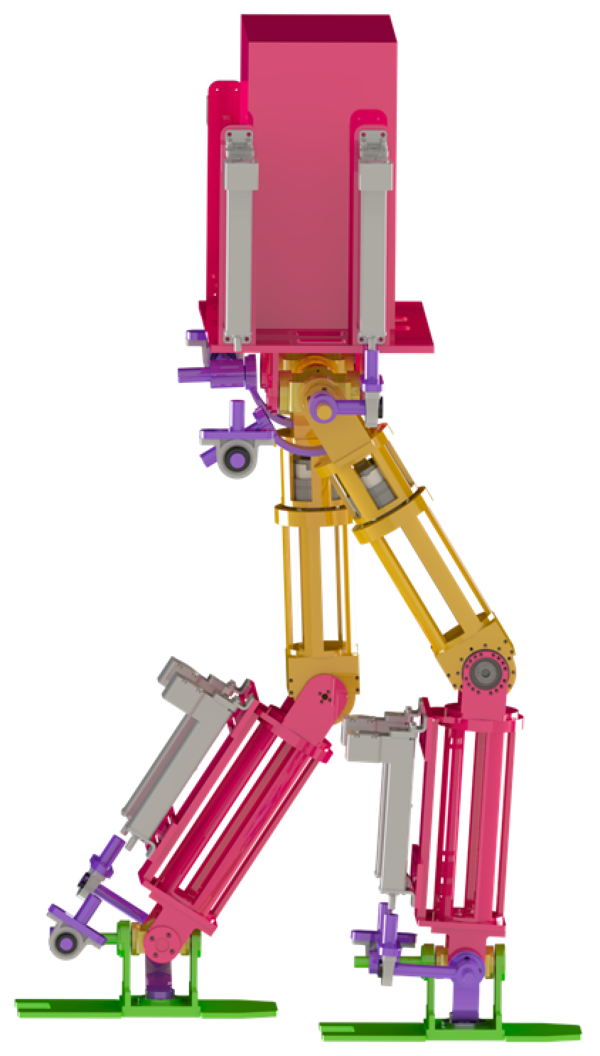
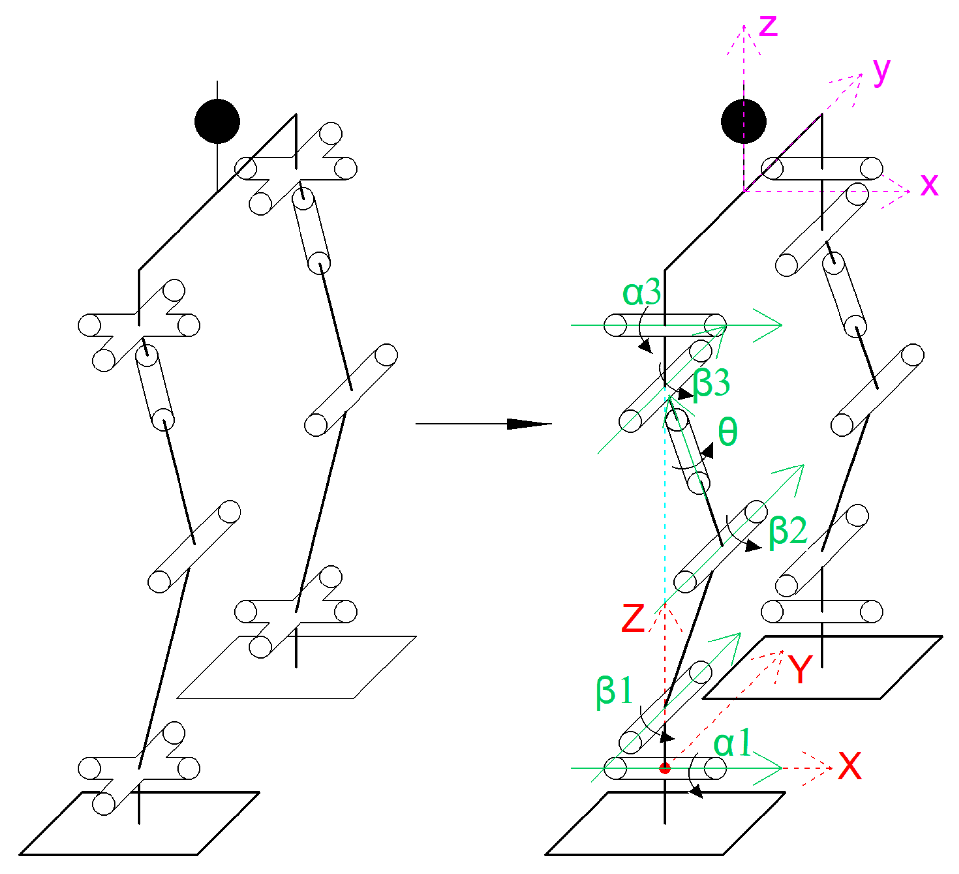
In this paper, the forward and inverse kinematics models of the new hybrid mechanical leg is established, based on screw theory and the POE formula. In the case of offline planning, the linear inverted pendulum model is used to plan the trajectories of different gait stages [
17]. The calculation trajectory is derived using MATLAB software v.2023a, and the dynamics simulation is carried out using Adams software to verify the rationality of the mechanical leg configuration design, kinematics and dynamics models, and the robot gait planning, providing reference for the subsequent motor selection and optimization of the actual prototype.
4. Planar Walking Gait Planning
Current gait planning methods are mainly applicable to mechanical legs comprising series or parallel mechanisms, and there is no extensive research on hybrid structures. Due to the concentration of the robot mass in the upper half, the leg mass can be ignored and considered as an inverted pendulum model centered on the ankle joint. By using an inverted pendulum model, inertia can be fully exploited, making the robot’s gait more natural and reasonable. At the same time, it can reduce the effect of the driving torque of the ankle joint on the walking stability of the robot [
19,
20]. The smaller the torque of the ankle joint, the larger the stability margin of the robot’s gait and the more stable the gait. The ankle joint has two degrees of freedom in motion, so planning around it requires finding the trajectories of the forward and lateral gait separately. The forward gait includes the trajectories of three mechanisms, hip, knee and ankle, while the lateral gait includes the trajectories of two mechanisms, hip and ankle.
A complete gait pattern comprises an initial phase, an intermediate phase and a stopping phase. The mid-stage is periodic, while the start and stop stages require the speed of the swinging leg during lifting and falling to not be too high, in order to avoid excessive impact force on contact with the ground, causing jerking and affecting stability. Therefore, the gait is planned in three phases.
4.1. Mid-Step Gait Planning Based on Linear Inverted Pendulum
During robot movement, it can be simplified as a pendulum rod centered around the ankle joint of the supporting leg, ignoring the mass of the swinging leg. In a linear inverted pendulum, the center of mass does not move in the Z direction and always moves parallel to the ground. Therefore, only the coordinate changes in the center of mass in the X and Y directions can be solved.
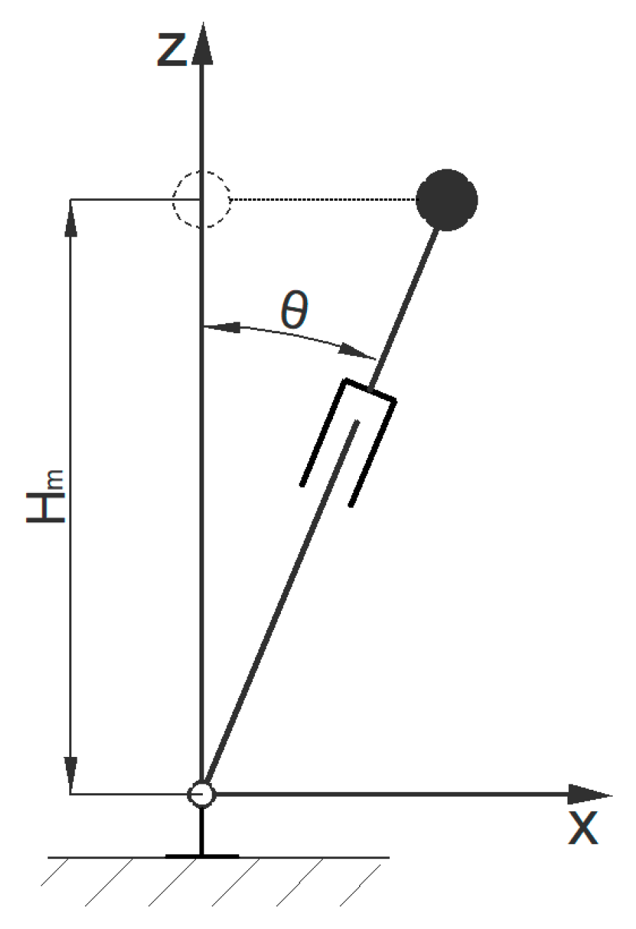
4.1.1. Forward Gait Planning of The Centroid
The forward gait model is shown in
Figure 3.
The equation of motion for an inverted pendulum is as follows:
The general solution of this equation is as follows:
According to the model, the relationship equation between the center of gravity coordinate and the length of the inverted pendulum can be obtained:
The single-step length in the periodic gait is set to
s, the time required for a single step is set to
Ts, and the bipedal support time is set to
Td =
Ts/4. The height of the overall center of mass relative to the ankle joint is
h. During the walking process of a bipedal robot, the motion of the legs is periodic and symmetrical; therefore, there are motion constraints:
Assuming that the moment when the centroid passes through the vertical axis is
Tm, the following can be obtained:
Based on these equations, the equations for the trajectory of the center of mass in the X direction are solved.
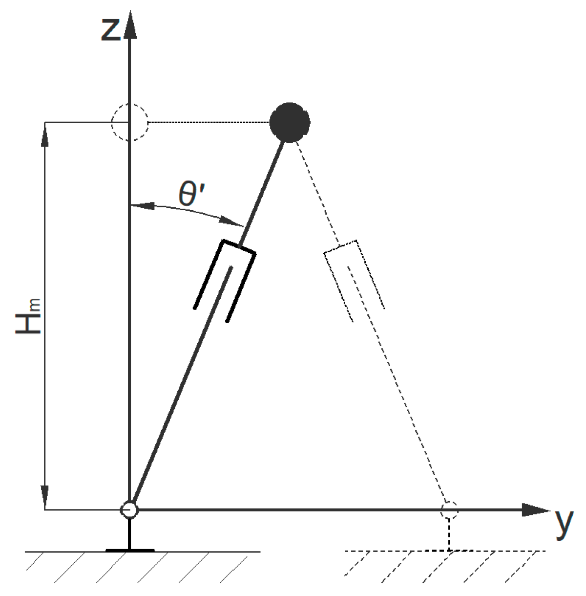
4.1.2. Lateral Gait Planning of The Centroid
In a lateral gait, there are alternating transformations in the inverted pendulum model. When the swinging leg and the supporting leg are in the same plane, the center of mass passes directly above the supporting leg, and it is specified that the lateral motion system time
t = 0 (when the lateral model system time is 0, there is a difference of one
Ts/2 from the forward model system time of zero). In lateral motion, the velocity of the center of mass is 0. When the system time
t =
Ts/2, the inverted pendulum model is in the state shown in
Figure 4.
According to the geometric relationship of the model, the motion constraints are set as follows:
When the system time is [
Ts/2,
T], the inverted pendulum model changes from the position shown in
Figure 4, and the supporting leg and swinging leg alternate. The displacement change in the center of mass is symmetrical with the motion state within [0,
Ts/2].
The equations of motion for the lateral model can be obtained from Formula (4) in the same way. Based on the equations of motion with the above constraints, the equation of the trajectory of the center of mass in the Y direction can be solved.
4.1.3. Forward Gait Planning of The Swinging Leg
The trajectory planning of the swinging legs is usually represented by the trajectory of the ankle position. Landing on the foot will cause some degree of impact and affect stability. Polynomial interpolation is used in the calculation to avoid the risk of impact and to ensure a smooth velocity change curve.
In the mid-stride phase, there is an alternation between the single and bipedal support. In general, the swinging leg lands and the start of the mid-stride cycle is when it enters bipedal support. At this point, the forward gait system time t = 0 is taken as the bipedal support phase time Td of the single-step cycle. Due to the symmetry of the leg movements, it is only necessary to plan a single-step gait to obtain a full-cycle gait. An XYZ coordinate system is set up at the projection point of the ankle joint of the support leg, with the X axis as the forward direction and the Z axis vertically upwards.
During the bipedal support period, if the position of the swinging leg remains unchanged in the
X direction, the motion constraints within the system time [0,
Td] can be obtained as follows:
During the single-leg support period, i.e., within the system time [
Td,
Ts], according to the motion conditions and positional requirements of the swinging leg, its motion constraints can be expressed as follows:
Based on the above equation, the equation for the trajectory of
x can be solved as follows:
In the Z direction, the sole must reach its highest point in the middle of a single step. Due to the symmetry of the single-step motion trajectory in the Z direction, the trajectory during the single-step support period is divided into two stages for planning, namely lifting and falling, from the moment at which the swinging leg passes the highest point.
During the bipedal support period, the swinging leg does not change in the
Z direction, i.e., within the system time [0,
Td], the following relationship can be obtained:
When the swinging leg is in the lifting process, i.e., [
Td,
Tm], the motion constraints can be obtained as follows:
When the motion constraint relationship of the swinging leg is opposite during the falling process, the trajectory of the change in the Z-coordinate of the swinging leg can be obtained:
4.1.4. Calculation of Joint Angles Based on a Generalized Coordinate System
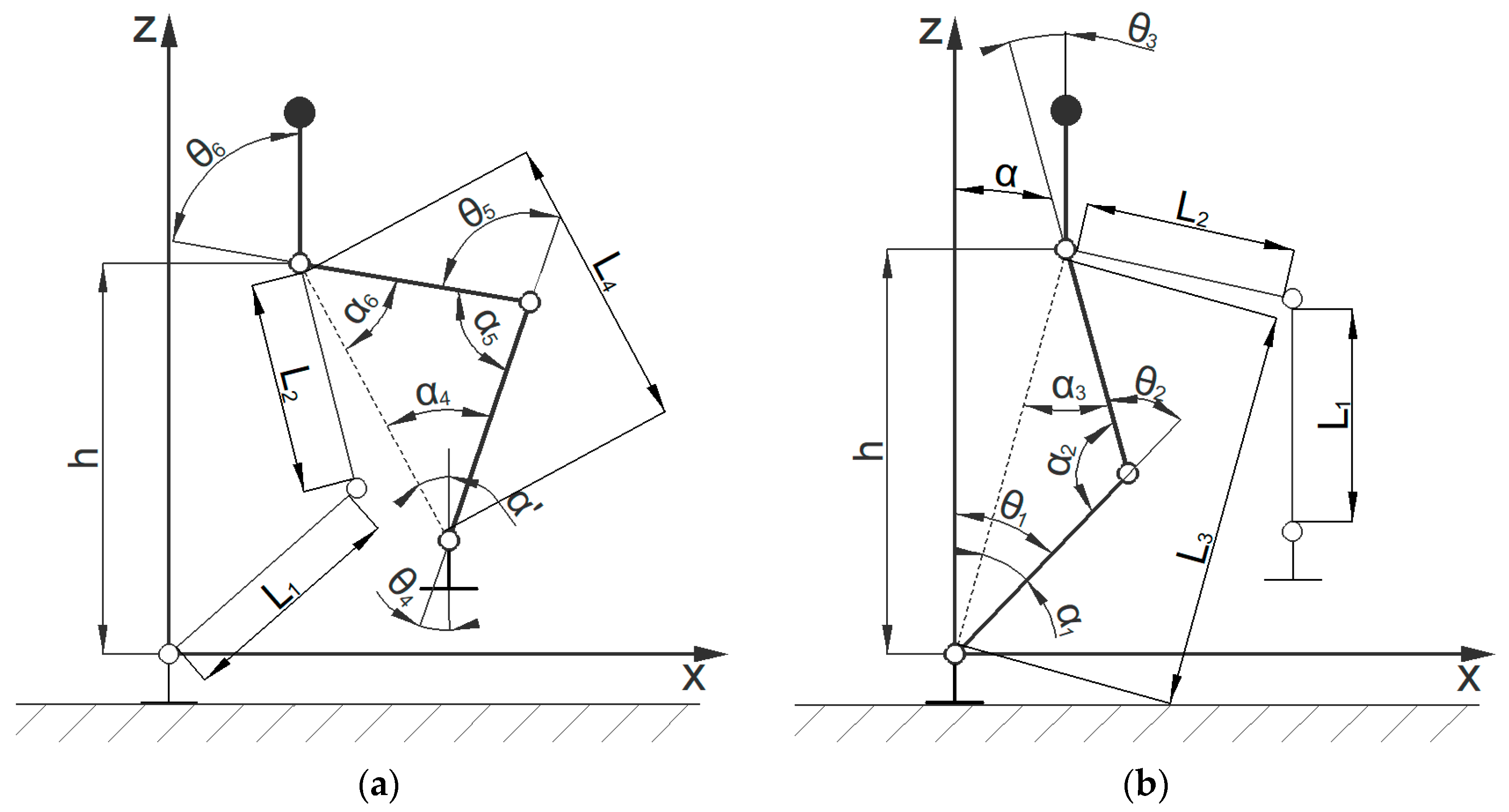
After obtaining the centroid motion trajectory and swinging leg motion trajectory, the angle changes in each joint can be obtained based on generalized coordinates. Based on the structural characteristics of the bipedal robot, the state of the legs at a certain moment in the mid-step gait is simplified to obtain the angle states of each joint between the swinging leg and the supporting leg, as shown in
Figure 5.
Given the centroid trajectory (
xm,
zm), let the distance from the centroid of the bipedal robot to the hip joint be
lm, with a thigh length of
l2, and a calf length of
l1. According to the geometric relationship in the figure above, the following equation can be obtained:
The angle relationship of each joint can be obtained via the generalized coordinate system, as follows:
Similarly, based on the relationship between the ankle joint motion trajectory (
x,
z) and the centroid motion trajectory (
xm,
zm), the following equation can be derived:
The trajectory of each joint of the swinging leg can be derived as follows:
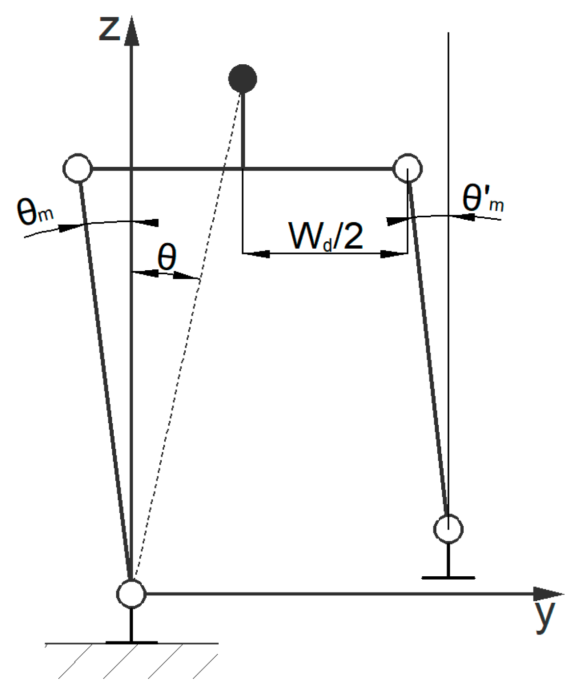
In a lateral gait, the robot’s upper body and foot soles are always parallel to the ground, and the knee joints have no lateral motion degrees of freedom, which can simplify the robot model, as shown in
Figure 6.
The generalized coordinate trajectory of the center of mass is (
ym,
zm), the vertical distance between the center of mass and the hip joint is
lm, and the distance between the centers of the two soles of the bipedal robot is
Wd. Based on the geometric relationship, the following equation can be obtained:
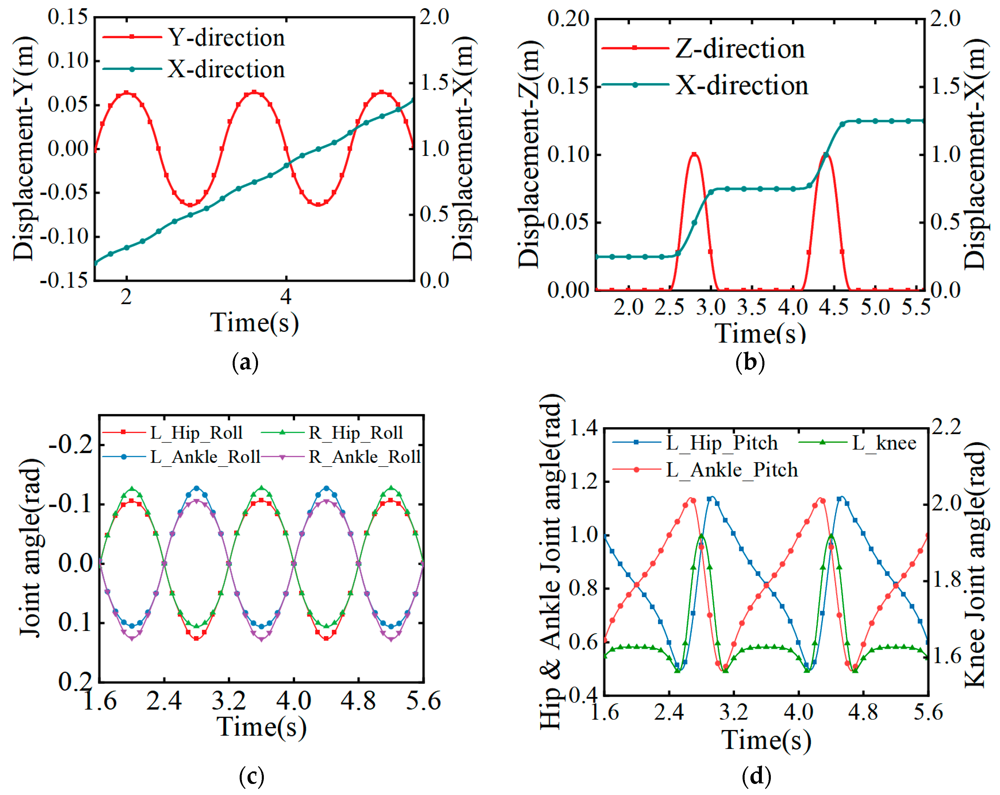
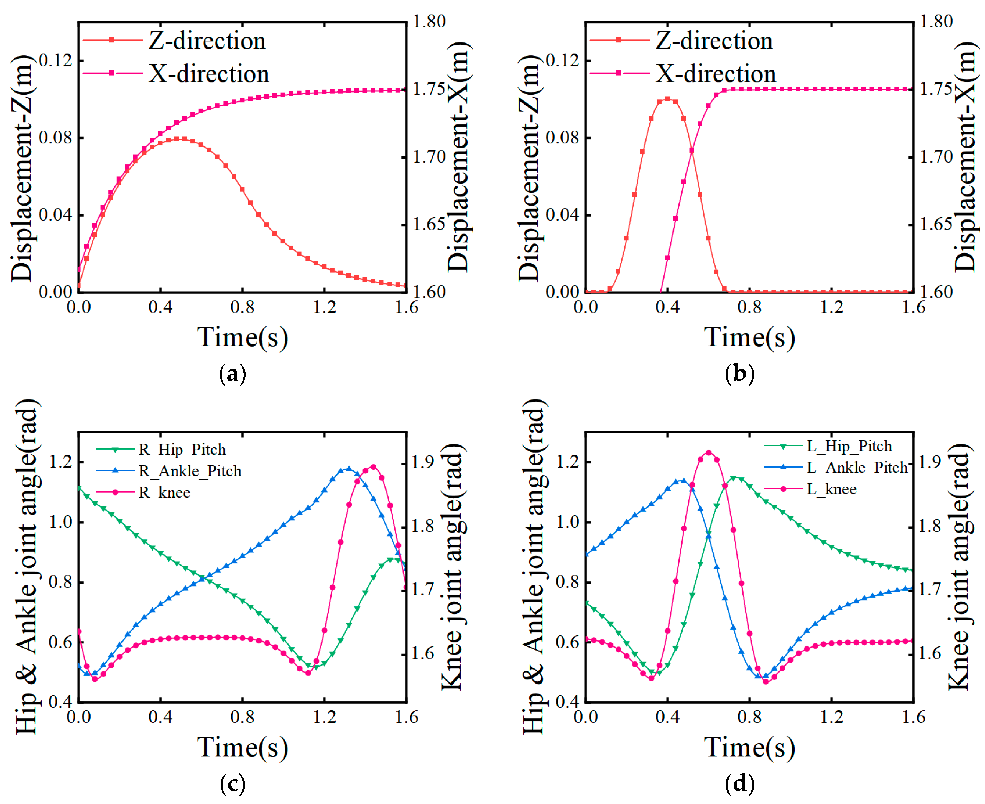
4.1.5. Mid-Step Gait Planning Results
In summary, the gait of a bipedal robot in a periodic mid-step gait can be obtained as, shown in
Figure 7.
4.2. Starting Gait Planning
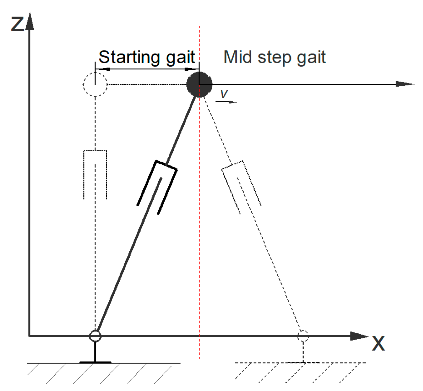
4.2.1. Trajectory Planning of The Centroid
The starting stage is a transition state from the static to the intermediate stage, from static balance with zero displacement and zero speed to dynamic balance. The attitude during the transition is shown in
Figure 8. According to the travel requirements of a linear inverted pendulum, and considering the energy loss caused by joint gaps, accuracy, and other factors, it is necessary to reduce the center of gravity to allow the robot enough space to adjust its joint angles during travel. Due to the differences between the robot’s motion model and the inverted pendulum model during this process, dynamic relationships are used to plan the starting stage.
In the
X direction, the motion of the center of mass deviates significantly and there is a possibility of instability. Therefore, in order to ensure a smooth connection between position and speed, the following motion constraints exist for the
X direction:
In order to maintain the balance of the motion process, when the deviation in the projection point of the center of gravity increases, the acceleration should also increase. Therefore, the acceleration in the
X direction is planned by using a quadratic function. When
t =
Ts, the center of gravity deviates the most severely, thus assuming the following:
According to the ZMP calculation formula, the following equation can be obtained:
Based on the above equation, the equation for the trajectory of
X can be solved as follows:
The lateral model motion state in the start phase also has similarities to the mid-step phase, so it is only necessary to use a correction function for the lateral joint angle change in the mid-step phase.
4.2.2. Trajectory Planning of Swinging Leg
The motion posture of the swinging leg during the starting stage is similar to that of the mid-step stage, with an initial bipedal support period. The difference is that the initial position of the swinging leg is different, and the starting point of the system time is different. Therefore, within the system time [0,
Td], there are the following motion constraints:
Within the system time [
Td,
Ts], there are the following motion constraints:
Based on the above equation, the equation for the trajectory of
X can be solved as follows:
The change in the trajectory of the swinging leg in the
Z direction during the starting phase can be obtained via polynomial interpolation (see
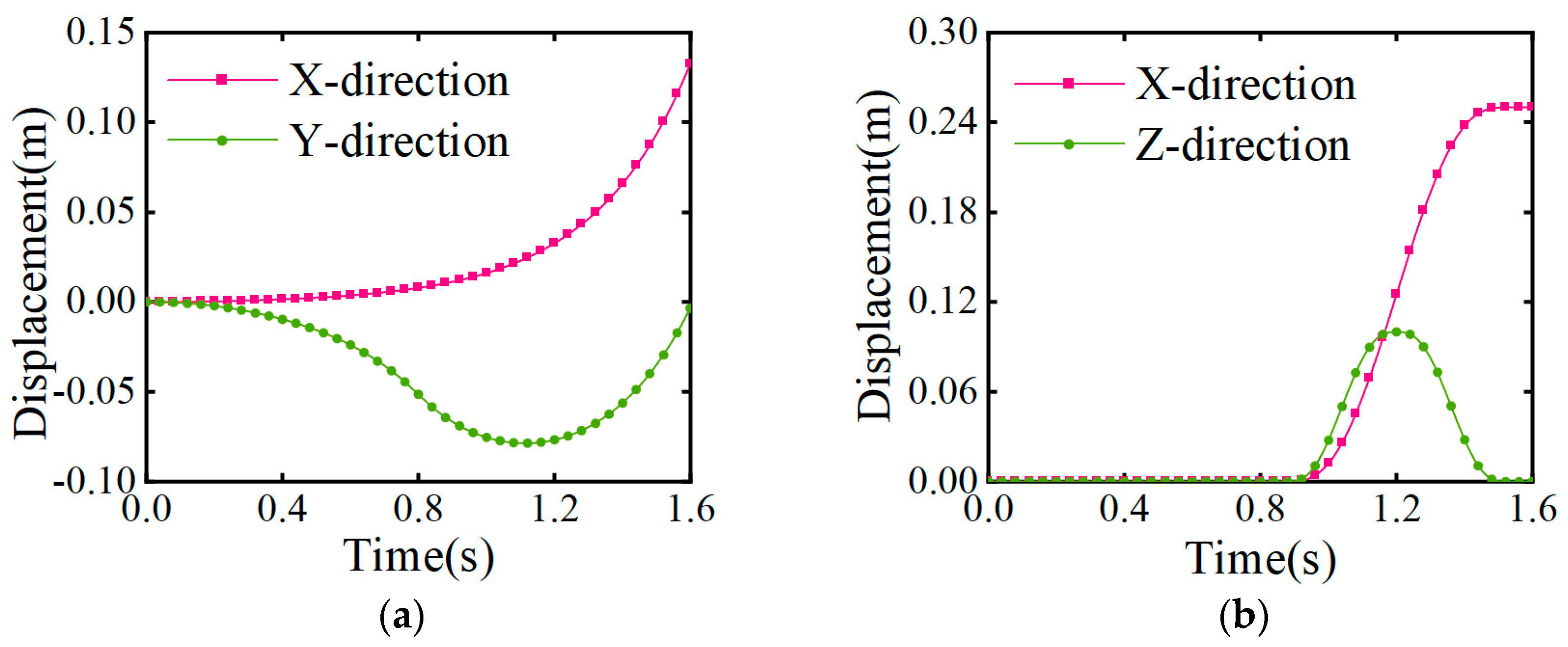
Section 4.1.3). In summary, the center of mass and the swinging leg motion trajectory during the starting stage can be obtained, as shown in
Figure 9.
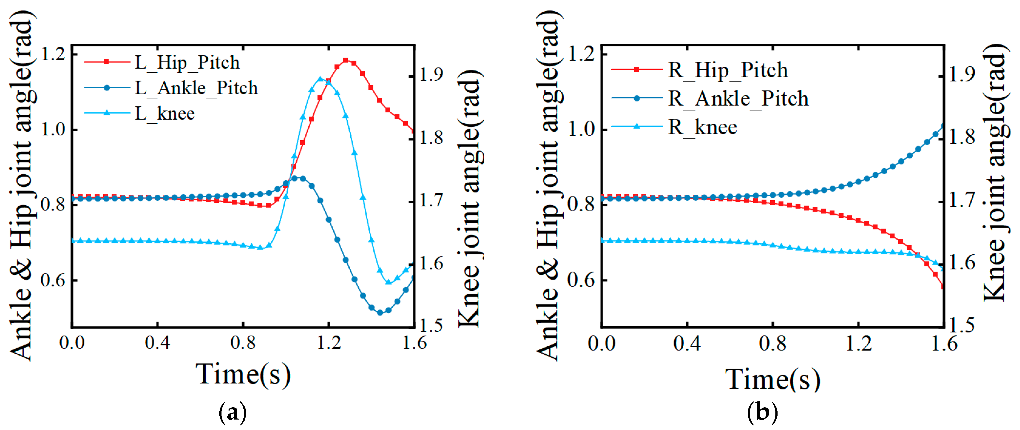
According to the generalized coordinate trajectory calculation of the joints of the support leg and swinging leg in the forward gait mentioned earlier, the motion trajectory of the joint angles of the support leg and swinging leg in the starting stage can be obtained, as shown in
Figure 10.
4.3. Stopping Gait Planning
The motion characteristics of the stopping stage are similar to those of the starting stage, with the difference being that their initial and ending states alternate with each other. Therefore, based on the symmetry of bipedal walking, the motion constraints of the stopping stage can be inferred from the gait of the starting stage. From this, the trajectory of the center of mass during the stopping stage can be obtained, as shown in
Figure 11.
5. Results and Discussion
As shown in
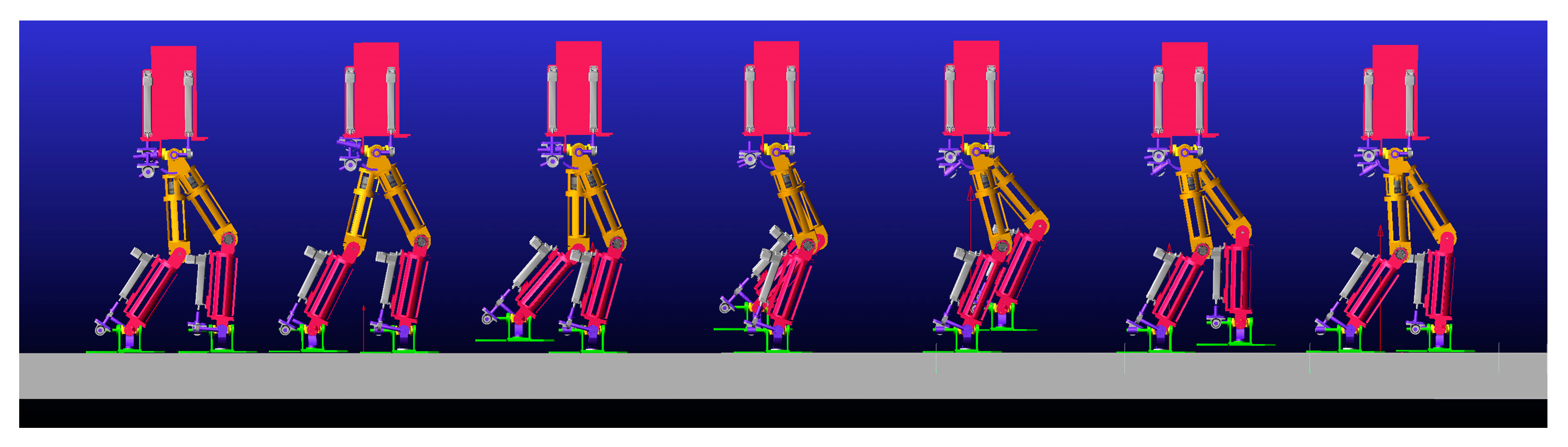
Figure 10, simulation experiments were carried out in Adams software for a bipedal robot walking on flat ground. According to the design requirements, the overall mass of the robot was 100 kg. The two simulation experiments were conducted by importing the discrete points of the robot joint angle trajectory curve via simulation software. The first simulation had a single-step length of
s = 0.25 m, a single-step period of
t = 0.8 s, and a simulation end time of 8 s. The second simulation had a single-step length of 0.5 m, while the rest remained unchanged. The robot walking sequence is shown in
Figure 12.
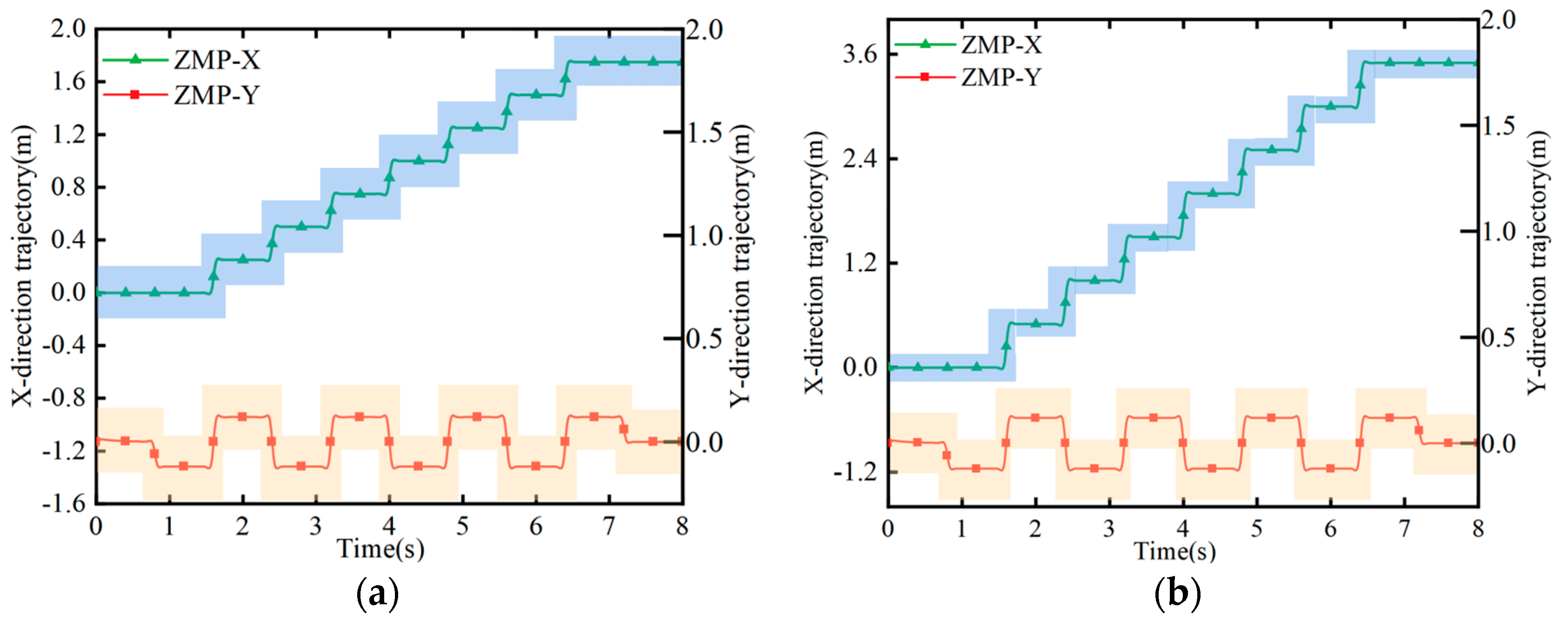
According to the simulation, the actual ZMP trajectory was obtained, as shown in
Figure 13. ZMP is a commonly used method for determining the stable state of the walking motion of bipedal robots. The definition of ZMP can be obtained from the literature [
21,
22]. Usually, when the ZMP is in the sole support region of a bipedal robot, the motion state of the robot can be considered stable. In theory, the trajectory of the ZMP is stepwise. However, according to the observation in the figure, the actual ZMP curve formed a smooth curve. In actual walking, if the ZMP is always in the position of the bipedal support domain, the robot’s walking is stable and will not overturn [
23].
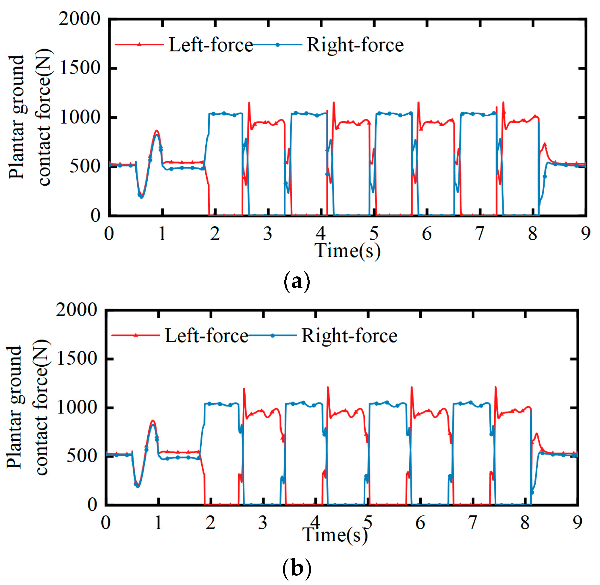
At the same time, the change in the contact force between the soles of the bipedal robot and the ground during the simulation process was obtained, as shown in
Figure 14. The change in the contact force was measured before the bipedal robot started squatting, and a slow squatting motion was completed within 0–1 s in order to achieve the required position of the center of mass. The contact force changed due to the acceleration and deceleration process of the center of mass. Within 1–2.6 s, due to the lack of Z direction movement in the center of mass, there was no significant change in the contact force within 1–1.8 s, followed by a left-foot start. In the mid-step gait, there was a significant alternating change in the contact force at the bottom of the feet. During the bipedal support stage of the mid-step, the two decreased and increased, respectively. When the contact force underwent a sudden change, it was the swinging leg landing and hitting the ground that met expectations and fluctuated within a reasonable range.
6. Conclusions and Future Work
This paper mainly analyzes the kinematics and dynamics modelling of the mechanical leg of a new hybrid bipedal humanoid robot, and plans and simulates the gait of the robot walking on the ground. The main results are as follows:
- (1)
Based on the new hybrid humanoid robotic leg, motion analysis was performed and kinematics and dynamics models were established, which enabled the planning of the gait, and laid the foundation for the subsequent application and research of the humanoid robotic leg.
- (2)
Gait planning of the robot walking on flat ground was performed, and the linear inverted pendulum model was used to plan the trajectory of the robot’s center of mass motion. The joint trajectory of the swinging leg was fitted using a quintic polynomial interpolation method to obtain a stable gait for each stage of the complete walking cycle.
- (3)
Using MATLAB and Adams to simulate a bipedal robot, the feasibility of the hybrid mechanical leg configuration design and gait planning was verified, laying the foundation for real machine experiments and providing a reference basis for the optimization of subsequent prototype structures, the selection of drive motors, sensor layout, etc.
The proposed gait planning method is suitable for robot walking at low speeds (less than 2–3 km/h). Future research should establish a set of control methods to prevent errors between the reference and actual trajectory from developing, considering the potential effects of unmodeled errors and floor unevenness.


