1. Introduction
In the field of autonomous underwater vehicles (AUVs), bio-inspired solutions have been sought in the last three decades as a source of improvement in terms of propulsive efficiency and maneuverability. As a matter of fact, fishes and marine mammals are faster and nimbler than their robotic counterparts: AUVs turnabout radius is normally a multiple of the robot hull length, namely from two to six times, whereas a biological swimmer is capable to reverse its course without breaking, with a radius of curvature of the order of one third of its body length. The cost of transport, which measures the energy spent to cruise at a given speed, is also significantly lower for aquatic animals when compared to the state-of-the-art of modern nautical technology [
1]. Therefore, several prototypes of swimming robots have been manufactured by researchers worldwide in the last thirty years, and an extensive review is provided in [
2].
Despite the efforts made to pursue the considerable potential payoffs of marine animals’ locomotion, the performance of biological systems are still far to reach. Indeed, the possibility to emulate effectively the swimming modes developed by aquatic animals over thousands of years of evolution depends from the understanding of the fluid mechanics principles of swimming locomotion. In order to address this very ambitious objective, computational fluid dynamics (CFD) analysis represents an invaluable tool to investigate the propulsive performances of biological and bio-inspired thrusters.
According to swim mechanics, thrust force originates from the momentum transfer due to the interaction between the fish body and the surrounding water [
3]. Particularly, body and caudal fin (BCF) swimmers generate thrust by bending their tails and caudal fins following specific undulation patterns. BCF locomotion is further expanded in five swimming modes characterized by the percentage of the body involved in the tail undulations. Thus, carangiform and subcarangiform swimmers generate thrust by bending respectively half and the last third of their tails. The motion law commonly adopted by biologists and roboticists to model the shape of the tail as a function of time is Lighthill’s travelling wave, an harmonic function whose amplitude increases moving towards the caudal fin [
4]. On the other hand, in thunniform locomotion, thrust generation is mainly due to the caudal fin motion, where tail motion is mostly confined. Here, the fin traces an undulating path to adjust its angle of attack and prevent flow separation [
5]. Indeed, thunniform locomotion is the most efficient swimming mode in BCF locomotion.
As stated before, several prototypes of bio-inspired underwater robots propelled both by carangiform and thunniform locomotion have been designed by researchers in the last thirty years. In the literature, the most common solution adopted to manufacture a carangiform swimming robot consists of a sealed forebody hinged to a piecewise flexible tail embodying a multi-joint, open-chain mechanism driven by dedicated servomotors or by a single rotary actuator [
6,
7,
8]. A similar architecture has been employed to drive the caudal fins of thunniform swimming robots [
9]. When a multi-joint mechanism is adopted to approximate the tail undulation patterns of the aforementioned swimming modes, it results easy to prove that the links of the system oscillate following an harmonic motion law. As a result, the caudal fin, which coincides with the tail linkage end effector, performs an harmonic roto-translation called flapping, where the individual components of the resulting motion are oscillation functions characterized by different amplitudes but the same frequency, and a constant phase shift. When a flapping caudal fin is employed as the thruster of a bio-inspired underwater robot, the quantification of its performance in terms of thrust generation and propulsive efficiency is a fundamental issue in the design process. As a matter of fact, in order to size the robot actuation system, the propulsive loads generated by the fin must be known as a function of the geometric and kinematic parameters of flapping motion.
To this end, this paper presents a detailed investigation of the dynamic performance of a roto-translating foil predicted by means of computational fluid dynamics. Here, the fin is simulated as a stand-alone thruster and the numerical predictions allow a complete characterization of its propulsive behavior. Aside from comparative considerations, the analysis results can be also exploited to compute the dynamics of a swimming robot and size its driving systems [
8]. CFD analysis has been extensively employed in the field of biomimetics. In [
10], the authors performed a two-dimensional analysis on the base ornithopter configuration of an insect flying robot using commercial CFD codes: the results have yielded deeper insights regarding the influence of varying flapping frequency on critical flow metrics regarding adequate lift and thrust generation. Flying systems have been investigated also in [
11], where CFD methods have been employed to model the transitional aerodynamics of the variable camber morphing wing. Numerical simulations have been also exploited in the marine field to model the hydrodynamic performance of manta-like flapping [
12].
Unlike other papers on the subject, the goal here is to provide a comprehensive performance-oriented manual on rigid flapping thrusters, which could be exploited as a design tool. Moreover, this work advances novel considerations on the physical effects of each kinematic parameter and proposes new perspectives on the cause-and-effect relationships between the wake structure and the propulsive performance, under a broad range of kinematic conditions. The heave amplitude, in particular, was varied in an interval that has seldom been studied in the past.
The paper is organized in the following way:
Section 2 outlines the kinematics, introducing the fundamental expressions of the flapping motion and the parameters of interest. In
Section 3 the numerical setup of the simulations is presented, including the spatial and temporal discretization schemes, the turbulence model implemented and the special treatment reserved to moving boundaries. The results are collected in
Section 4, preceded by a brief description of the mesh and the definition of the main propulsive performance indicators. Finally, the most significant conclusions are drawn in
Section 5.
2. Motion Kinematics
Fishes and aquatic mammals arrived to their current locomotion capabilities through a process of biological optimization, driven by natural selection. As a result, a wide and complex variety of swimming behaviors have developed, usually classified into (i) undulatory, (ii) oscillatory, (iii) pulsatile jet-based and (iv) drag-based motions. For a detailed explanation of each class the interested reader can refer to Smits’ well-known review [
13]. The species adopting motion behaviors that fall within one or another of these categories further exhibit peculiar body shapes, with geometries and mass distributions that coupled with the adopted swimming configuration have the effect of optimizing their underwater motion.
A complete and exact representation of such a rich variety of configurations, if possible, would require the adoption of prohibitively complex models, rendering computational simulations unfeasible. However, it has been showed how for the oscillatory configurations, which include BCF swimmers, significant simplifications may be adopted and still derive a model retaining relevant information about the physics of the problem. For instance, various experimental investigations [
5,
14,
15,
16] showed that the approximation of the oscillatory regime through a flapping hydrofoil predicts the maximum efficiency in the same range of kinematic configurations found for cetaceans and carangiform fishes.
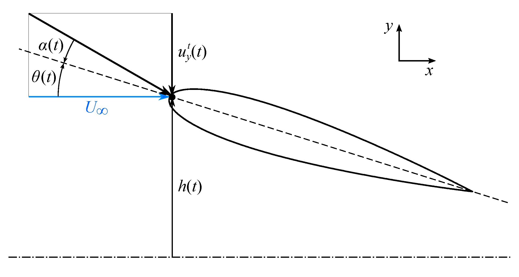
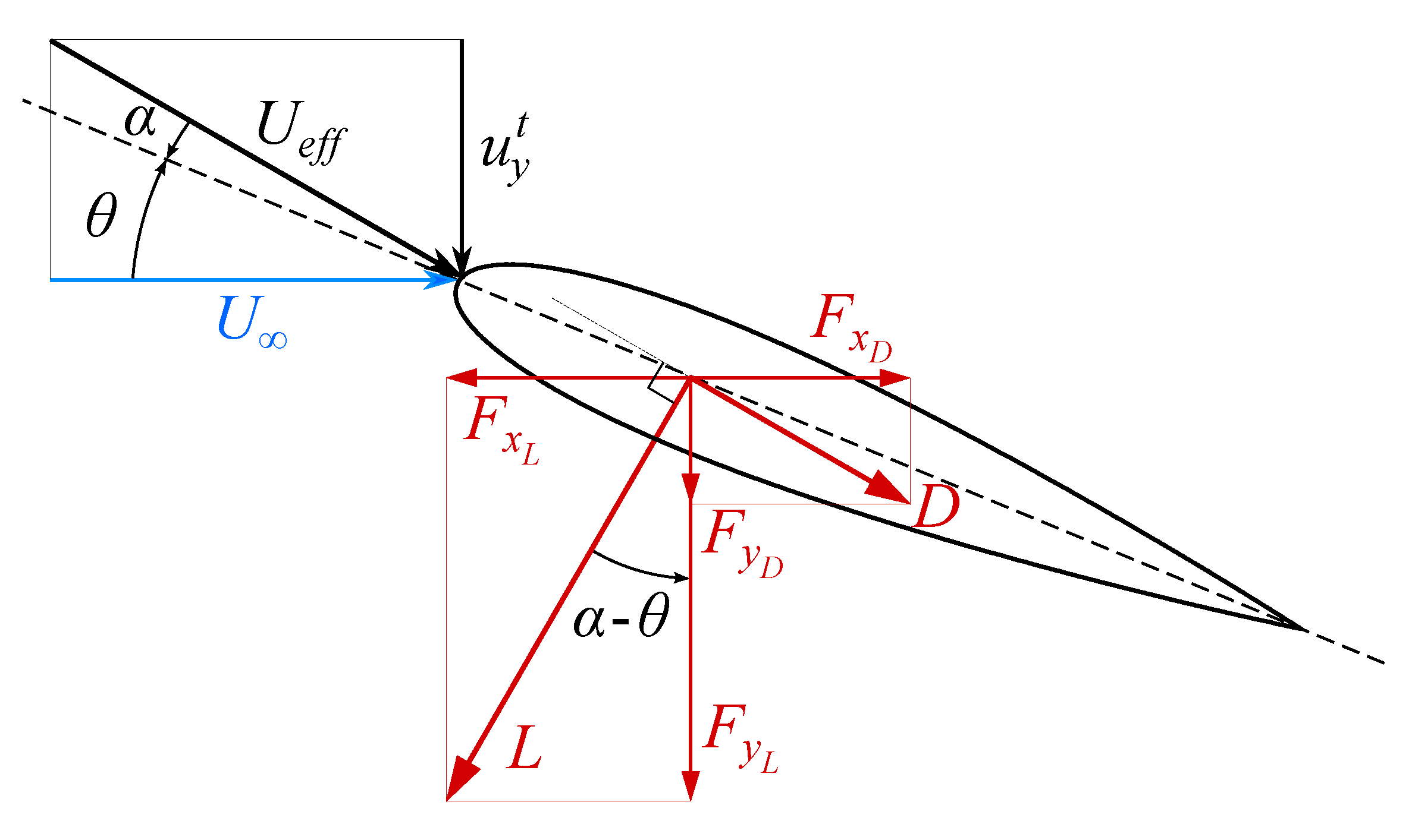
Within the flapping foil approximation, the body inertia contribution in the propulsion generation is discarded, with the motion assumed to be concentrated at the body end, namely at the propeller tail. The latter is then suitably approximated via hydrofoil profiles, moving according to kinematic laws approximating their natural motion. The analysis has here been restrained to a two-dimensional case, with the propeller approximated using a symmetric NACA0015 profile, whose schematic representation is given in
Figure 1 together with some relevant kinematic parameters.
The profile is hence prescribed to move according to an harmonic law composed of a rotation around a pivotal point and a vertical translation, following the parametrization presented below:
According to Equation (
1), pitch amplitude and vertical displacement follow a sinusoidal variation with frequency
f. The pitching motion occurs around a fixed center of rotation, with the maximum angular displacement given by
. The simultaneous heaving motion is characterized by an amplitude
and present, with respect to the periodic rotation, a constant phase shift
.
From the above relations, the vertical and rotational velocities may be read as:
where the superscript ‘
t’ identifies the components representing the relative motion between the inertial and the moving reference frames. The velocity induced by the profile vertical motion affects the instantaneous, effective angle of attack, that according to the convention exposed in
Figure 1 may be expressed as follows:
with
being the horizontal free-stream velocity. The maximum value reached by
in the harmonic period is indicated by
.
A global description of the profile kinematics widely adopted in the topic of flapping hydrofoils is provided via the Strouhal number
This non-dimensional parameter groups together the profile oscillation frequency with a length scale that best characterizes the flow. In the context of flapping foils the characteristic length may be associated to the wake width A, here approximated by the total heave amplitude .
The predominance of heaving or pitching in the foil motion can be quantified by means of the dimensionless heave ratio, defined by Akoz et al. [
17] as
where
is the time instant at which the trailing edge (TE) reaches its highest vertical position and
is the total vertical excursion of the TE. The motion is heave-dominated when
, while
identifies a pitch-dominated kinematics.
In order to provide a comprehensive analysis of the propulsive performance related to the flapping motion, a wide range of kinematic configurations have been explored. Thrust and efficiency have been computed for several combinations of , , and , which have been extensively recognized as the major kinematic factors influencing the propulsive capabilities of the foil.
3. Simulation Setup
As far as the numerical framework is concerned, the simulations were carried out adopting an incompressible, high-order discontinuous Galerkin (DG) solver. This DG solver was extensively validated over the years for a broad variety of fluid dynamics applications [
18,
19,
20,
21]. The current implementation with a moving reference frame was validated in [
22] for a flow past a transversely oscillating cylinder, where the numerical resuts were compared with well established reference data.
The problem has been modelled adopting as governing equations the fully turbulent Unsteady Reynolds-Averaged Navier-Stokes equations (URANS), equipped with the Spalart-Allmaras [
23] one equation model for the turbulent viscosity-like variable
. Such choice has been motivated by the widely demonstrated efficacy of this particular one-equation model in aerodynamic flow predictions, also showed in the framework of oscillating foil, reported for example in [
24,
25]. The validity of the Spalart-Allmaras turbulence model to simulate oscillating foils in a DG environment was addressed in a recent paper [
26], where the numerical results showed good agreement with the experimental data available in literature.
To avoid dealing with moving meshes a relative reference frame, fixed with the NACA profile, is introduced. The governing equations are then formulated expressing the velocity components
defined in the absolute (inertial) frame described in terms of the coordinates in the moving frame [
27,
28]. The relative motion between the two frames is then represented by an inter-frame velocity vector
. The vectors
and
, introduced in Equation (
2), are now to be intended as expressed in terms of the foil-fixed relative frame coordinates, with
representing the distance vector from the rotation point and
being the Levi-Civita tensor. In this way it is easy to see that
exactly identifies the profile velocity, as seen from the inertial frame, projected onto the relative one.
Exploiting the solenoidality of the velocity field
, the equations of motion assume the following form:
where the working variable for the pressure is to be intended as the specific pressure
and
d is the minimum distance from the wall. The effective turbulent viscosity is derived as
, with
, as well as
and
, being a closure function that, together with the constants
,
,
and
, defines the Spalart-Allmaras model. The interested reader may find a comprehensive description of the previously cited terms in [
23].
The numerical scheme is constructed starting from a suitable partition of the physical domain
, where the exact solution of the above model lives, into a set of
non overlapping elements
:
The DG discretization is then obtained by considering an element based, modal expansion for the solution vector making use of base functions made up by hierarchical, orthonormal polynomials up to order n. The analytical solution is hence locally approximated via a finite-dimensional, piecewise-continuous polynomial, possibly discontinuous across element interfaces.
For the sake of compactness the state variables are collected in a solution vector
so that the equations above may be represented in the following matrix notation:
Here the term
, where
denotes a single entry matrix, has been introduced to cancel the time derivative of pressure in the continuity equation, keeping the model consistent with the representation provided in Equation (
6). Finally,
and
identify the convective and diffusive flux tensors, both function of time and system state, while the vector
, introduced to collect the source terms, contains the contributions of the non-inertial components arising from the inter-frame formulation.
In this way, the modal Galerkin expansion for the vector
reads:
where
defines the number of degrees of freedom, the function
identifies the
i-th component of the polynomial base, and
collects the corresponding degrees of freedom of the solution vector. The index
k, instead, takes into account the element-based character of the method, with the base functions
having compact support.
Having a local approximations of the solution vector living in the polynomial space ensures a space accuracy of order for the velocity and eddy viscosity-like, and order of accuracy n for the pressure.
The numerical scheme is then constructed passing through the variational formulation of the above system of partial differential equations. Defining a test function
, living in the same finite-dimensional vector space of the solution vector, the weak formulation is obtained imposing an orthogonality condition among
and the governing equations and integrating by parts:
where the element index,
k, in the integrand functions has been dropped.
One of the key features of a DG method consists in the evaluation of a uniquely defined, normal, numerical fluxes
, depending on the adjacent elemental states and gradients. The convective flux,
, is here treated using the artificial compressibility flux method reported in [
29], while for the viscous contribution,
, the well-known BR2 discretization scheme of Bassi and Rebay [
30] is implemented.
Introducing in Equation (
10) the previously defined
n-th order modal expansion for
finally yields a system of linear ordinary differential equations (ODEs) for the global degrees of freedom (d.o.f.) vector
Q:
where
is a modified global, block diagonal mass matrix, characterized by null entries at the pressure degrees of freedom,
is the global solution vector containing the solution d.o.f. and
is the residual vector, containing the surface and volume contribution of flux tensors and non−inertial source terms.
The system is discretized in time using a three-stages, third-order accurate Rosenbrock-type Runge-Kutta scheme ROS3P [
31]. The latter is of linearly-implicit type, it allows the construction of the new time solution
by freezing the Jacobian matrix
computation at each time step, avoiding hence any non-linear resolution procedure. The linear system arising from time discretization of Equation (
11) is finally resolved using a flexible generalized minimal residual (GMRES) solver preconditioned by a highly parallel efficient
p-multigrid algorithm, described in [
32]. It should be underlined that due to the inter-frame velocity formulation, the boundary condition are non-homogeneous and the system is in turn non-autonomous, with a d.o.f. time dynamics that results to be function of not only the state vector but also, explicitly, of time.
4. Results
This section gives a brief description of the computational grid and introduces the main results in terms of flow fields and propulsive performance plots. The latter have to be intended as an integration of what was partially presented in the CFD analysis contained within the multiphysics study performed by Costa et al. [
8].
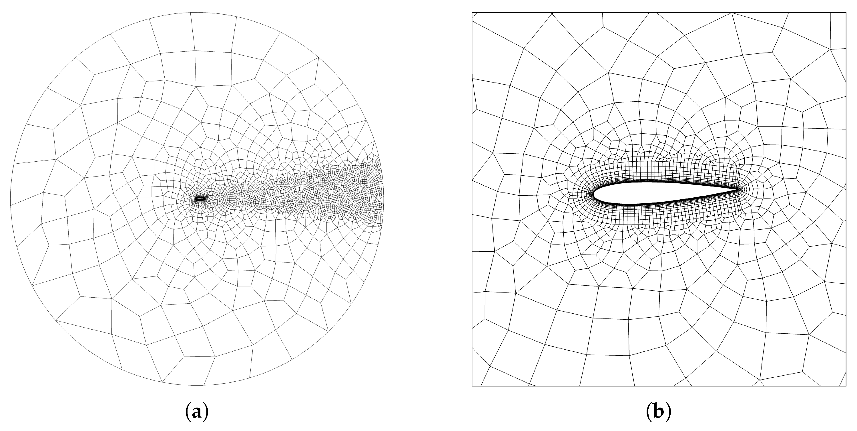
The fluid domain is a circle of radius
, where
c is the foil chord length, discretized by means of an unstructured mesh with
quadrangular elements, as illustrated in
Figure 2a. The Open Source software employed for the mesh generation is GMSH [
33]. The cells nearby the boundary of the profile are structured-like and adequately curved so to wrap around the foil curvature, as shown in
Figure 2b. The face of these cells is approximated using a piecewise third order polynomial. The cells in contact with the profile have a height
and get progressively inflated outwards for a total of 19 layers. The region behind the foil is refined to enable an accurate study of the wake, which is directly correlated to the propulsive features of the flapping motion. In particular, it is well known that the forward motion of a flapping foil is characterized by counter-rotating eddies forming a jet-like wake, typically denoted as reverse Von Kármán vortex street [
34]. In order to verify the independence of the results upon the mesh we did not follow a grid refinement procedure, typical of low-order methods, but rather a check increasing the polynomial degree of the solver, as done in [
26], which is known to be a viable alternative for high-order schemes. Simulations were carried out up to
.
The reason was just to ensure the convergence of the results, as a matter of fact the propulsive performances remained practically the same once
was reached, see for example the performance data reported in
Figure 3a. The time integration was done with a step size ranging from
to
. The choice was driven by the need to obtain a satisfactory trade-off between numerical stability and computational expense.
For the sake of generality, the forces in
x and
y-direction, i.e.,
and
, and the torque
exerted on the foil are normalized, ending up with the drag, lift and moment coefficients below
where
is the fluid density and
b is the (unit) span. It should be noted that the force components
and
, together with the torque
, are to be intended as expressed in the absolute reference frame, meaning that the referred
x and
y-direction coincide with the two coordinate axis of the inertial frame.
The propulsive performance associated to the oscillating motion is evaluated in terms of mean thrust coefficient
and propulsive efficiency
. Essentially, the assessment is based on the amount of propelling force that the foil is able to produce per unit period and on the effectiveness of this production mechanism in relation to the power spent to activate the body. In mathematical form the two quantities can be defined as
where
is the mean power coefficient
while
and
T represent the number of cycles selected for the average and the period, respectively.
All the kinematic configurations addressed in this paper are featured by a Reynolds number
. As reported in [
26] this value is enough to employ a fully turbulent model, as for flapping foils the latter provides results analogous to those obtained using an algebraic transition model. This holds true as long as there is no combination of extremely small
and high
, which is not present in any of the simulated cases. The center of rotation of the foil is located inside the profile, along the chord line, at
from the leading edge. Since the aim was to analyze the sensitivity of the propulsive performance to the kinematic variables discussed in
Section 2, a series of tests were performed by changing just one parameter and keeping all the others constant. The choice of the test cases was made starting from a known efficient flapping configuration typical of BCF swimmers, characterized by
,
,
and
. The kinematic parameters in play were then varied between lower and higher values for a reasonably extended interval, in order to include a representative number of operational conditions.
Table 1 collects the complete list of cases and the resulting propulsive efficiency and mean thrust coefficient. The graphical version is given by
Figure 3,
Figure 4 and
Figure 5. Moreover,
Figure 6,
Figure 7 and
Figure 8 depict the vorticity fields of the majority of the cases contained in
Table 1. Indeed, despite someone remarks that there is no one-to-one connection between the wake morphology and the propulsive performance [
13], the visualization of the vortical structures surely helps in understanding the physical mechanisms that improve thrust and/or efficiency. Some of the kinematic configurations have been also animated over few cycles, in order to study the shedding of the vortices during upstroke and downstroke with greater detail. These animations are provided as
Supplementary Materials.
In the following paragraphs the effect of each kinematic parameter is isolated and dissected.
4.1. Angle of Attack and Dynamic Stall
Numerous works recognized the angle of attack as a crucial parameter to control the propulsive performance of a flapping foil [
15,
35,
36].
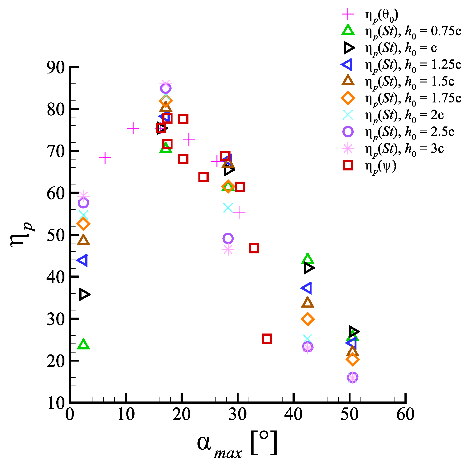
Figure 9 presents a compact portrait of the entire space of configurations simulated, plotted in terms of propulsive efficiency against maximum angle of attack.
Even though efficiency is affected by the interplay of all kinematic parameters, a global optimum is always identifiable, for the explored configurations, in correspondence of those generating
between
and
. This is in fair accordance with what reported in [
36], but even so high values of efficiency are still found for
values falling well above the static stall condition.
Due to the circulation-based aspects of the considered propulsion mechanism, the persistence of high efficiency at elevated
suggests the presence of a continuous production of lift that might be traced back to the onset of dynamic stall process [
37,
38]. Dynamic stall is a complex phenomenon affecting airfoils in conditions of unsteady motion. It determines a delay in severe separation, enabling the profile to produce lift up to angles of attack well above the static, stall-inducing value. Within the considered framework of flapping kinematics, the contribution coming from the aforementioned unsteady motion manifests as a time-dependent rate of change in the angle of attack
. With its shape and magnitude intimately dependent upon the tested motion parameters, such quantity proved to be of fundamental relevance, being involved, in particular, in the control of some of the dynamic stall aspects critically affecting the profile propulsive performances, see
Section 4.3.
As the dynamic stall regime sets in, imposing a dynamic delay of stall-like separation, a lift increasing tendency along with
is observed. This follows a rather complex behavior and is eventually characterized, for the larger values of
, by sudden increments owed to the arise of local separation phenomena and the subsequent vorticity organization at the solid boundary. These coherent structures, arising over the suction surface of the foil, are usually referred to as leading edge vortex (LEV), or also as dynamic stall vortex (DSV) in the specialized literature [
39,
40,
41]. Despite the significant lift increase that such structures have been demonstrated to provide, the obtained results seem to suggest how the optimal condition, from an efficiency viewpoint, is identified by configurations limiting, when not avoiding, their formation. Following the observations reported in [
39], the above assertion may be rephrased by saying that for a configuration producing large thrust efficiently,
should be in the so-called linear region of the
plane, found within the pre-stall regime.
In other words, analogously to steady aerodynamics, the peak angle of attack should be kept low enough so to avoid massive separation if one wants to produce thrust in an efficient way.
The authors are aware of the limitations related to the application of turbulence models to unsteady aerodynamic problems, particularly when accurate capturing of loads at large
and the onset of boundary layer separation are required. Nonetheless, the framework of URANS simulations, employing several closure equations among which the SA version used in this paper, proved its capability of yielding results qualitatively significant when investigating dynamic stall [
40].
For optimal conditions
should not be too small either. To clarify why one can refer to
Figure 10 and consider the following argument. For heave-dominated motions the power produced by the torque
has been observed to be much smaller than the one generated by thrust and drag. Indeed, in the computations reported here, its contribution to
is less than
and hence it can be neglected. With this hypothesis the instantaneous output and input power
,
are given by
with
. The propulsive efficiency is then computed as
From Equation (
18) it is easy to verify that
when
, due to the fact that
This means that as long as lift dominates drag, the efficiency is close to the unit regardless of the modulus of the lift and its orientation. Otherwise the efficiency starts to decay along with the lift-to-drag () ratio, due to the progressive emergence of the detrimental contribution of drag both in the streamwise and vertical directions; this comes as no surprise since the ratio represents the aerodynamic efficiency of a body. In this context the dependence of on , and thus partially on , even if it exists, is much less impactful. Since prior stall one can imagine that, for a symmetric profile in quasi-static conditions, , at very small angles of attack the lift is almost absent whereas the drag is not, being with . This leads to a very small ratio which determines not only a very small , but also an unsatisfactory .
4.2. Pitch Amplitude
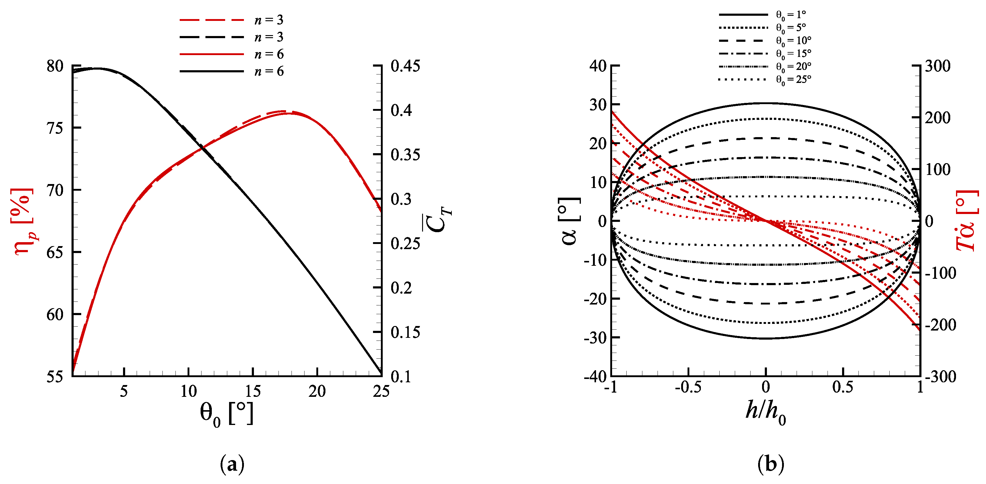
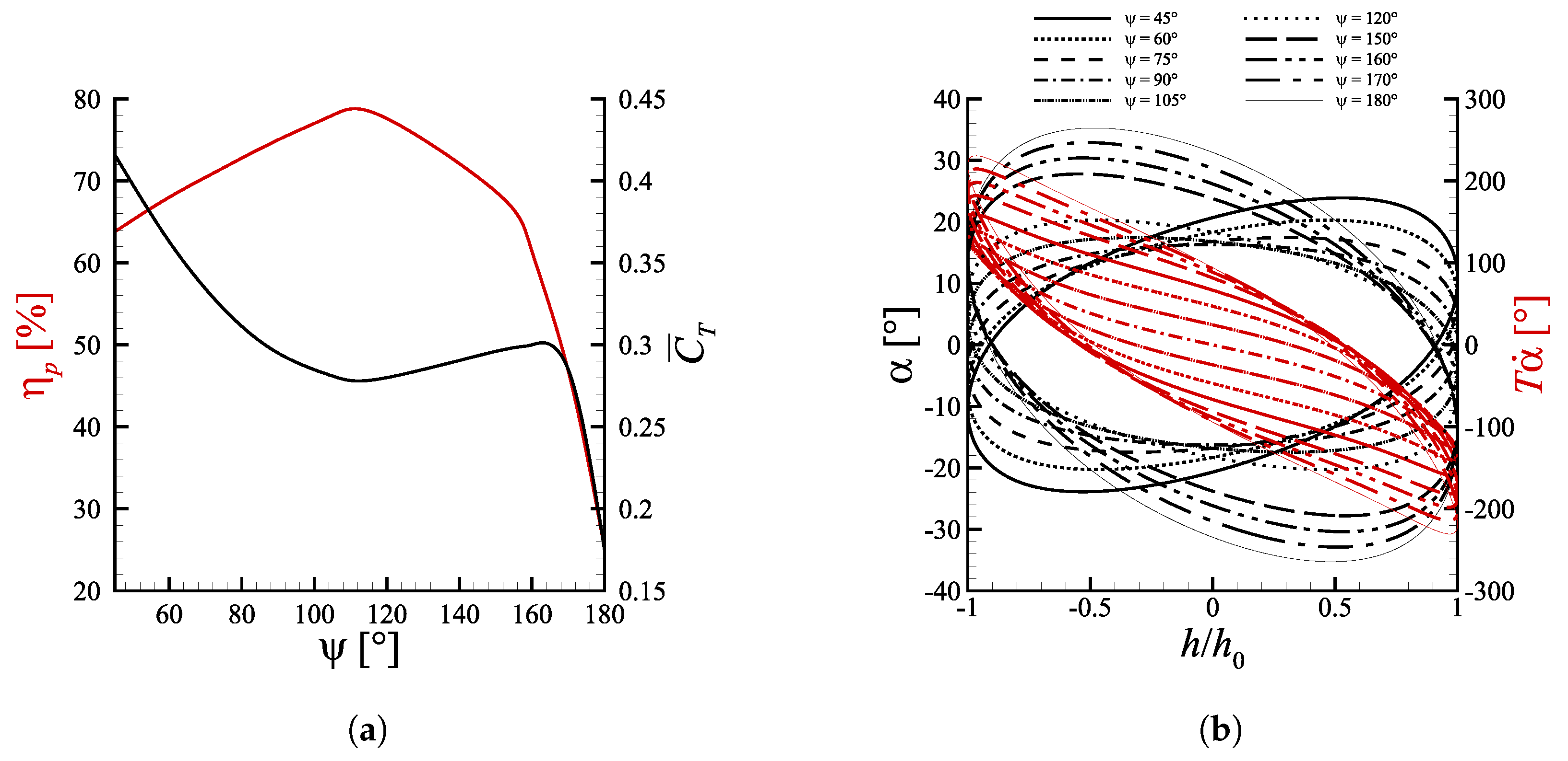
The pitch amplitude is also an important quantity, because it does not only set the maximum excursion of the pitch angle, but it also modulates the pitch rate.
Figure 3a displays the performance sensitivity to the pitch amplitude
, maintaining
,
and
. The pitch amplitude was varied using the stencil
. Note that the
was set to such value in order to get
for the reference case
,
,
, where
may be thought of as the ‘real’ Strouhal number based on the TE total excursion.
The thrust coefficient presents a global maximum presumably within the interval
and quickly drops for greater values of total heave excursion. This is due to the progressive decrease of
as
is increased, which in the end brings the profile in a situation where lift is practically zero. The fact that the maximum mean thrust is produced at peak angles of attack over
may be explained again with the dynamic stall phenomenon, whose impact is amplified at low pitch amplitudes due to the higher rate of change of the angle of attack, as displayed by
Figure 3b. The maximum efficiency has a value of approximately
around
. To understand why efficiency is maximized in this region, one can recall what was said in
Section 4.1 about the dependence of
on the
ratio. The interval
is indeed where the ratio between lift and drag returns the highest value. For lower pitch amplitudes lift increases due to the dynamic stall effect, but drag increases even more and gives a lower
ratio. At higher pitch amplitudes, instead, the peak angle of attack is so small that lift is almost null, differently from drag which is non-zero even when
.
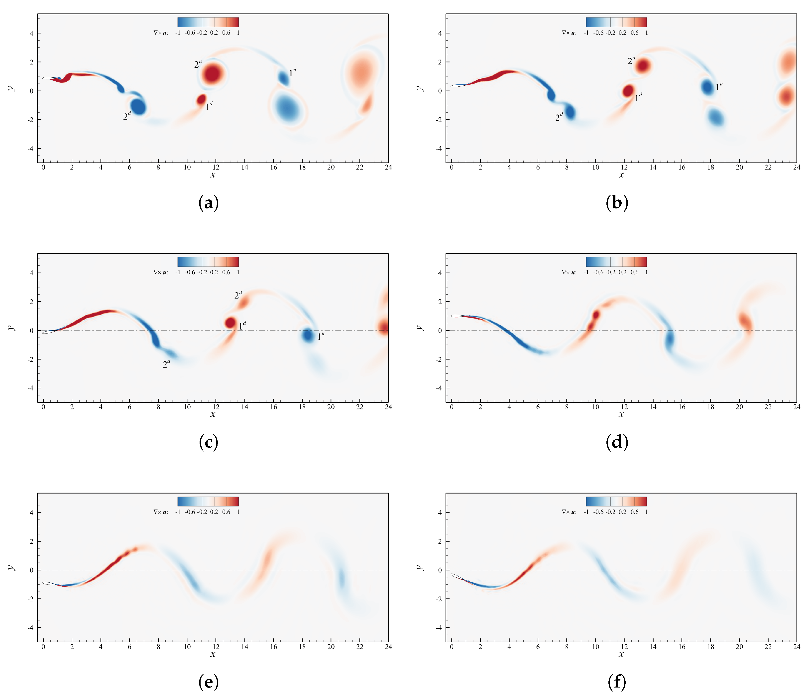
Figure 6 depicts the vorticity fields at varying pitch amplitude. Starting from
Figure 6a we can see a typical 2P wake, in accordance with the nomenclature introduced by Roshko and Williamson [
42]. The counter-rotating vortex pairs shed each half cycle are not balanced though, as the second vortices generated during upstroke/downstroke (indicated with
/
in
Figure 6a) are much bigger than the corresponding first ones (identified by
/
). As
increases, the second vortices lose strength and at
they become less intense than their counterparts, which seem to maintain instead the same size and level of vorticity (
Figure 6b,c). Further increasing
the second vortices start to be fragmented in multiple co-rotating swirling structures and become so weak that they merge almost immediately with the first vortices, leading to a sort of 2S wake which resembles a reversed von Kármán street. Above
the instantaneous angle of attack always remains well below the value of static stall, therefore clear separation cannot be appreciated and no vortex gets formed downstream the foil, with the wake being basically streamlined. An interesting insight could be extracted by noting that the vortex pairs observed up to
seem to be formed in two distinct phases. The first vortices are created at the extremes of the heave motion, where
is maximum, and detach when the foil is approximately in the neutral position, meanwhile the second eddies arise past the centerline, where
reaches its maximum value, and detach when the profile approaches the point of maximum vertical displacement. This could suggest that
,
are linked to the separation owed to the reaching of an angle of attack greater than the stall value, whereas
,
are caused by the sudden change of
rather than its instantaneous value, as it can be appreciated in
Figure 3b. On the base of this assumption
,
would be nothing but the so-called starting vortices largely examined in literature [
39]. Since the second vortices origin on the side of the foil opposite to where the profile is moving (lower surface in upstroke and upper surface during downstroke) their effect is beneficial in terms of thrust production, because they rotate contrarily to a classical von Kármán street. On the other hand, the first vortices rotate in the opposite sense, and so their contribution is detrimental or beneficial from a propulsive point of view, depending on the timing of the detachment. Specifically, if
(
) detaches below (above) the certerline it most likely has a positive effect on thrust generation, otherwise it acts in drag favor. The positive or negative effect of the vortices depends indeed not only on the sense of rotation, but also on the position with respect to the neutral axis (see
Section 4.4 for a more detailed motivation).
The fact that for small pitch amplitudes
is larger, especially around
, produces stronger second vortices and allows to obtain high
. This, in turn, helps to maintain efficiency at discrete levels. On the base of these reasonings one could argue that the efficiency is decently high even when the second vortices weaken as in
Figure 6c, despite the first vortices maintaining the same strength as cases at smaller
. The explanation could be traced back to the fact that when
,
becomes less energetic,
,
detach slightly earlier and as a consequence they move upwards (downwards) in downstroke (upstroke) switching their role from detrimental to beneficial in terms of propulsive performance averaged over the entire period.
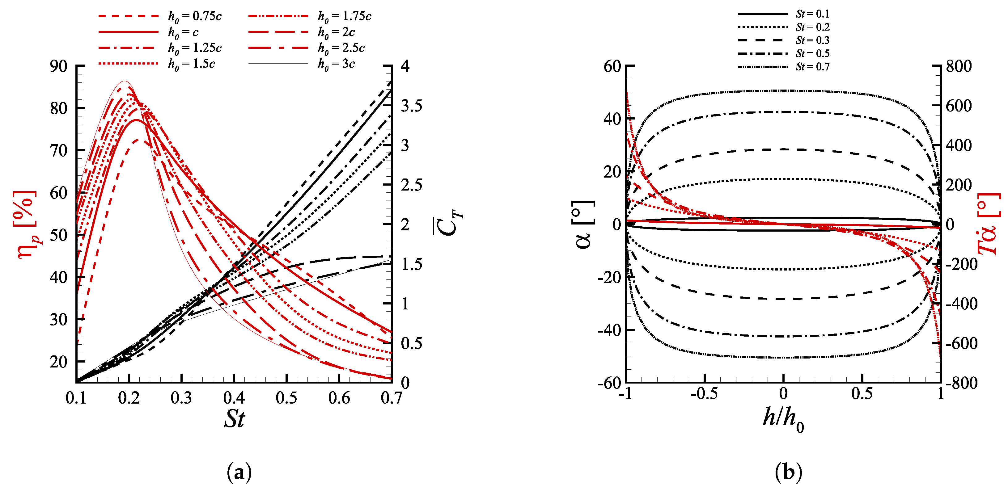
4.3. Strouhal Number and Heave Amplitude
In
Figure 4a, the combined effects of Strouhal number and heave amplitude are portrayed, keeping fixed
and
. Note that by maintaining constant pitch amplitude and phase shift, the configurations characterized by the same
number produce the same
, as one can write
with an effect of the heave amplitude corresponding just to a direct modulation of the motion period
, with
being the time scale of the flow. Equation (
20) hence shows that, for a fixed
, the term
does not depend on the heave amplitude, see also
Figure 4b, and in particular as
is increased
decreases and vice versa.
The maximum efficiency manifests over a neighborhood centered in
, with a peak value above
for
at
. The fact that for all heave amplitudes
occurs in such range is in line with what was documented in [
5,
15,
43] and reflects the assertion advanced in [
14,
16,
44,
45], namely that most fishes swim following this flapping frequency, which corresponds to the most efficient from a propulsive standpoint. The mean thrust coefficient monotonically increase along with
due to the continuous increment of lift owed to the onset of dynamic stall effects, as already mentioned in
Section 4.1.
Another distinctive feature, detectable in
Figure 4a, is the significantly different effect of heave amplitudes on the propulsion performance at small and large
. As far as
is concerned, the cases with
, which have the highest
, present the best efficiency at low
. After such optimum,
decreases very fast moving towards higher Strouhal numbers, with the configuration
becoming the least efficient after
. These findings confirm what reported by Akoz et al. [
17], according to which heave-dominated motions maximize their efficiency at low Strouhal numbers. On the other hand, the configuration
, generating the least optimal efficiency among the ones that have been investigated, exhibits the most subtle
decrease at high Strouhal numbers, demonstrating to be the most efficient one when high angles of attack are involved. An almost identical trend might be observed in the
curves. As a matter of fact when the Strouhal number is low the mean thrust coefficient is maximum for
, instead at high
the propelling force is optimal for
. An helpful insight on such dynamics might be extracted from the visualization of the phase diagrams reported in
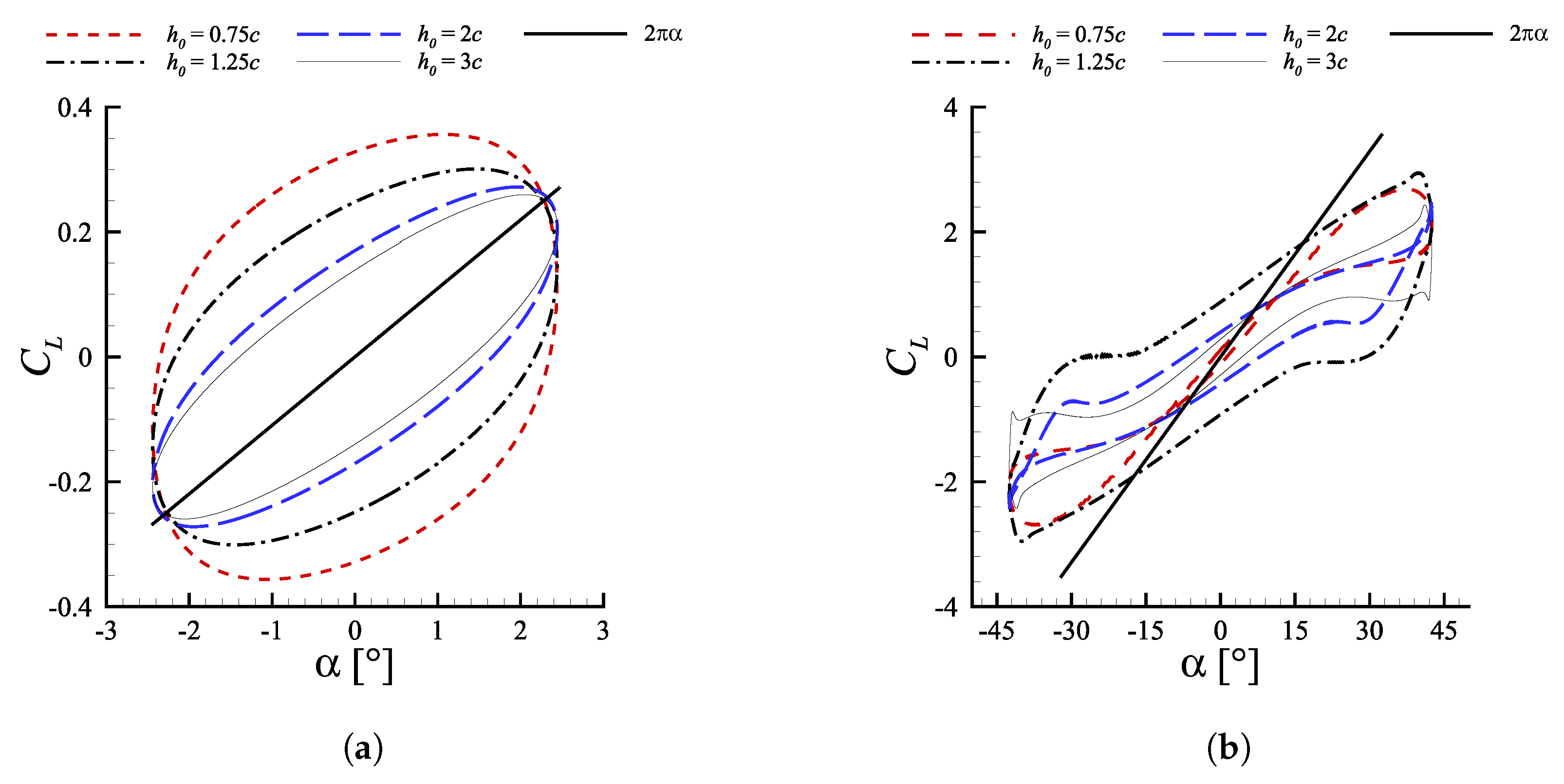
Figure 11. Therein we consider the lift coefficient defined as
against the values assumed by
during one motion period. Two cases, in particular, are analyzed as they show an opposite behavior with respect to the heave amplitude: (i)
and (ii)
.
At
a motion regime for which
is established. Due to low angles of attack, the effects of stall delay coming from a fast dynamics are not triggered, with the latter seeming to mainly induce strong energy-loss features. This is reflected in
Figure 11a by the presence of a distinguishable reduction of the hysteresis cycle as
is increased. Such progressive collapse of the
curve appears to produce an alignment with the
law, characteristic of steady, inviscid aerodynamics.
On the other hand, as the Strouhal increases a parallel increment of the
experienced by the profile during its cycle occurs. At
,
Figure 11b, a value
is reached as the profile pass through the zero vertical position. For such values of angle of attack, well above the static stall, the trend-inversion in the effects of increasing heave amplitude on the propulsion performances does not come as a surprise. Indeed, the beneficial effects of a fast dynamics, allowing for a separation delay and a continuous lift production result to be strongly mitigated when increasing
, due to the associated decreasing effect on motion frequency. Referring again to
Figure 11b, for the configurations with
the dynamic contribution coming from large
enables to keep generating lift up to
, reaching peak values after crossing the position corresponding to
, i.e., as the profile decelerates towards its maximum stroke displacement. Conversely, when
the reduction of
causes a decrease in the maximum sustainable angle of attack before occurrence of deep stall and thrust collapse. In particular, for
the lift coefficient experiences a sudden drop after a localized peak at
. Such behavior is consistent with the onset of a deep stall, featured by the presence of a chord-sized LEV arising from leading edge separation, before reaching
.
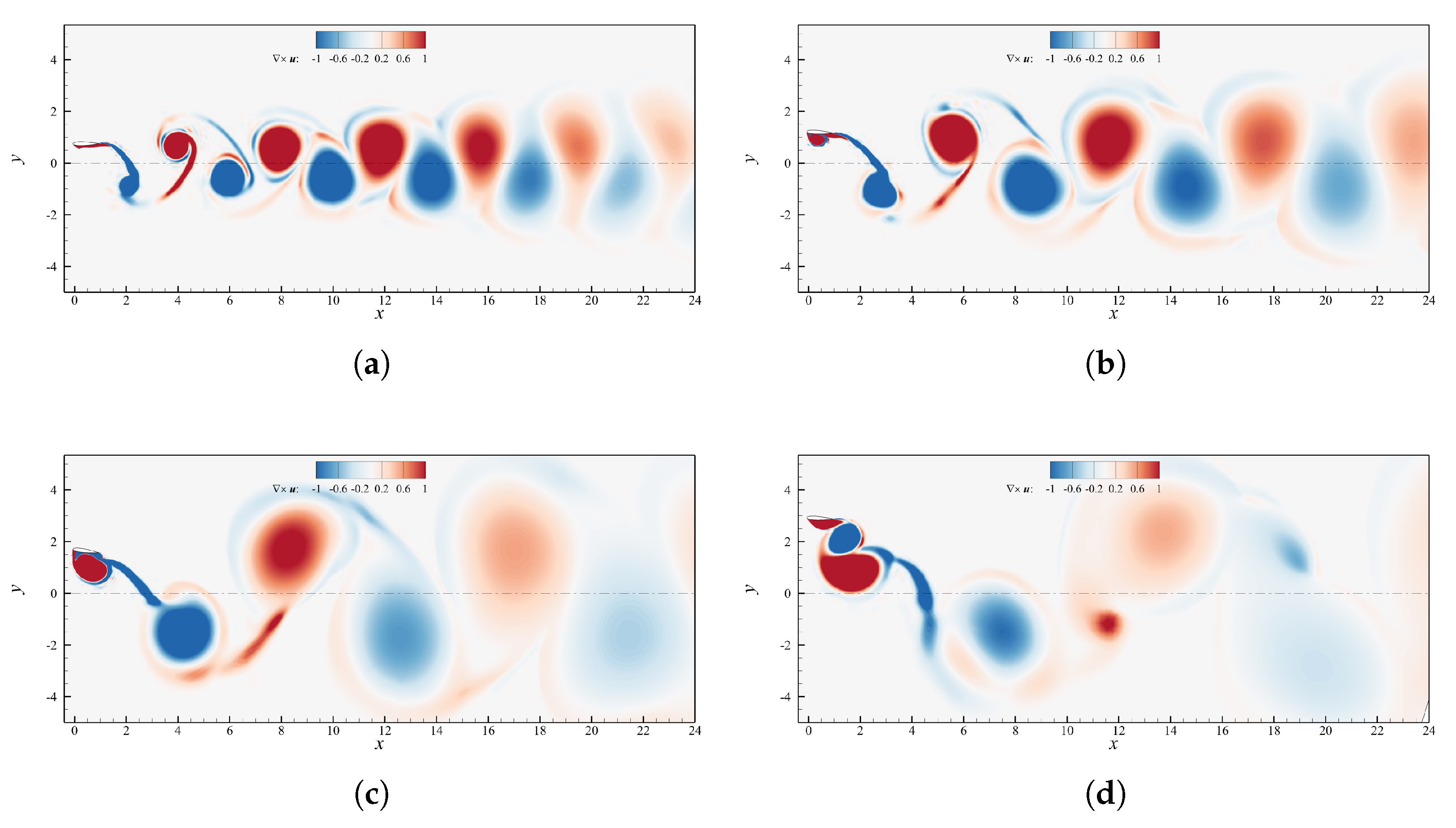
Figure 7 includes the vorticity fields at
for the values of
reported above. As
,
Figure 7a,b, both captured during upstroke, the frequency variation has a clear manifestation in the modification of the pattern of the shed eddies. In particular, for
the high motion frequency, inducing large
values, avoid significant leading edge separation as the profile travels through
while for
a distinct separated region of positive vorticity is clearly distinguishable. When
,
Figure 7c,d, a chord-sized LEV detaches from the solid boundary as the angle of attack approaches its maximum in the cycle, with the profile entering in deep stall. For
,
Figure 7d, a negative vorticity region close to the profile identifies the further shedding of a large trailing edge vortex (TEV). It might be conjectured, as also reported in [
39], that as the formed LEV detaches and starts being advected downstream, i.e., as the deep stall comes into being, the sudden change of pressure distribution around the profile forces the roll-up of the opposite vorticity boundary layer, creating the above mentioned TEV that, therefore, can be considered as a further sign of deep stall onset.
In conclusion, independently on the
regime at which the profile operates, it would seem that efficiency-driven propulsion solutions should mainly focus on kinematic configurations ensuring minimal, if not absent, leading edge separation. At low Strouhal this is guaranteed, provided an adequate choice of phase shift is performed, see
Section 4.4, by the low angles of attack that are produced, whereas when dealing with fast dynamics regime an effective thrust production, even though sub-optimal, requires low heave.
4.4. Phase Shift
The phase offset between pitch and heave sinusoids establishes whether the leading edge leads the trailing edge or vice versa.
Figure 5a shows the propulsion characteristics as function of the flapping phase angle. In this case
was varied between
and
with a constant step of
and between
and
with a step of
, keeping the remaining parameters fixed at
,
and
. This choice was made in order to include both the interval where efficiency have been reported as the highest [
35,
36] and the regions where
undergoes a considerable degradation.
According to Van Buren et al. [
36] the phase shift is a crucial factor, and this is corroborated by
Figure 5, where both
and
are subjected to large variations, in an interval that covers less than one-half of the entire spectrum of phases. The mean thrust tends to increase moving away from
due to the increase of the angle of attack, which increments the lift, nevertheless drag increases even more and causes
to diminish. Once
then
becomes too high and
collapses, producing in turn a drop of the efficiency. The cause is that
becomes insufficient to avoid deep stall at angles of attack greater than
. The phase shift, in fact, seems to have a rather bland effect on
(see
Figure 5b) and it does not allow to obtain values high enough to counteract the simultaneous growth of
. The efficiency is maximized at
, in between the results outlined by Van Buren et al. [
36] and what is predicted by linear theory, for which
verifies at
and
, respectively.The diverse behavior of efficiency and mean thrust coefficient at phase angles greater or lower than
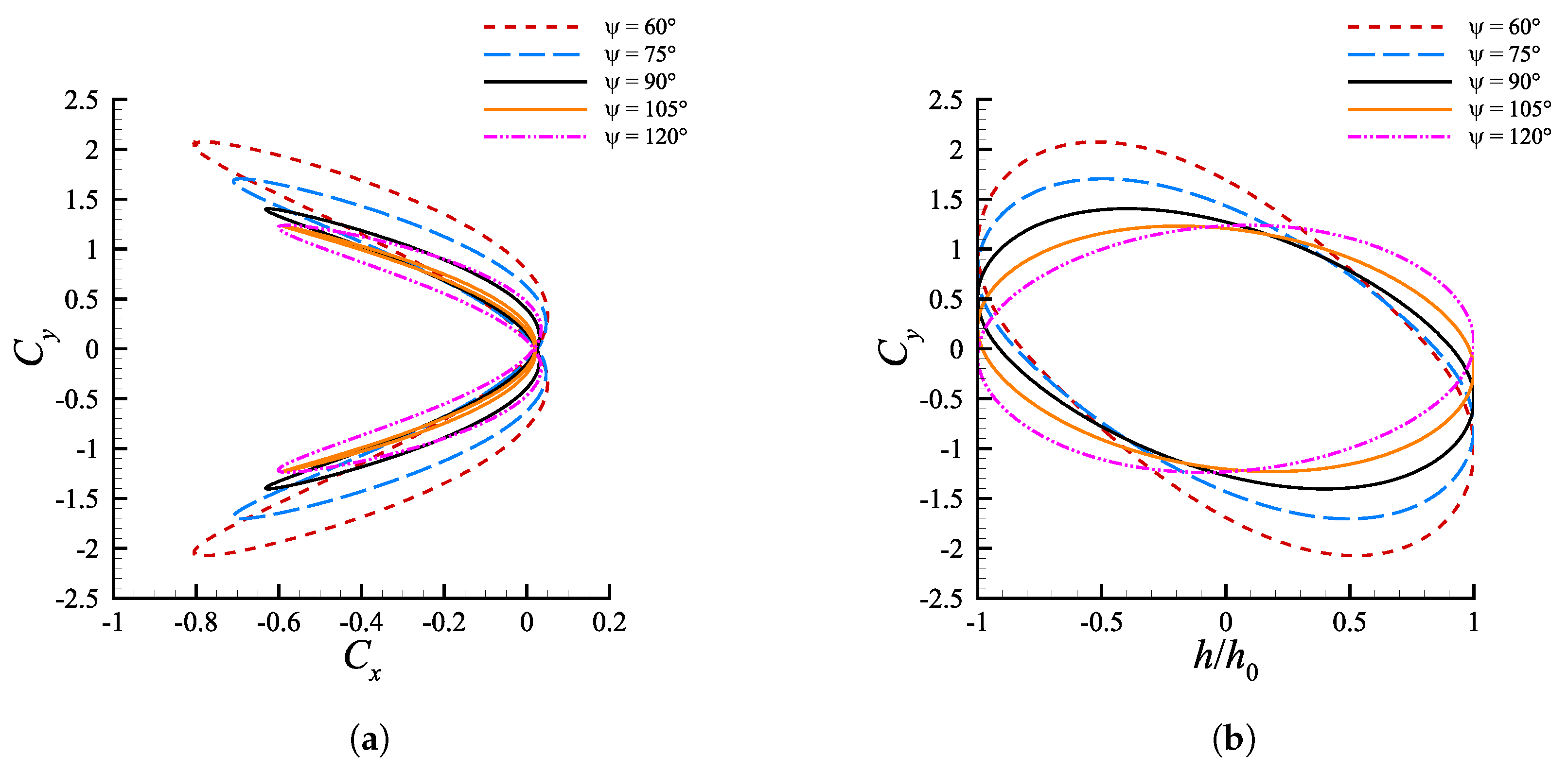
can be investigated looking at
Figure 12. Among the simulated cases, the efficiency is optimal at
because it allows to change the angle of attack in such a way to boost
in the first half of the upstroke and downstroke phases and diminish it in the second halves, as showed in
Figure 12b. This reflects in a minimization of the hysteresis in the
space (
Figure 12a), which is directly linked to
as pointed out in
Section 4.3. Aside from the hysteresis one can also note in
Figure 12a that for
the thrust coefficient reaches higher values throughout the oscillating cycle (we recall that
), whereas for
the orbits span between smaller values.
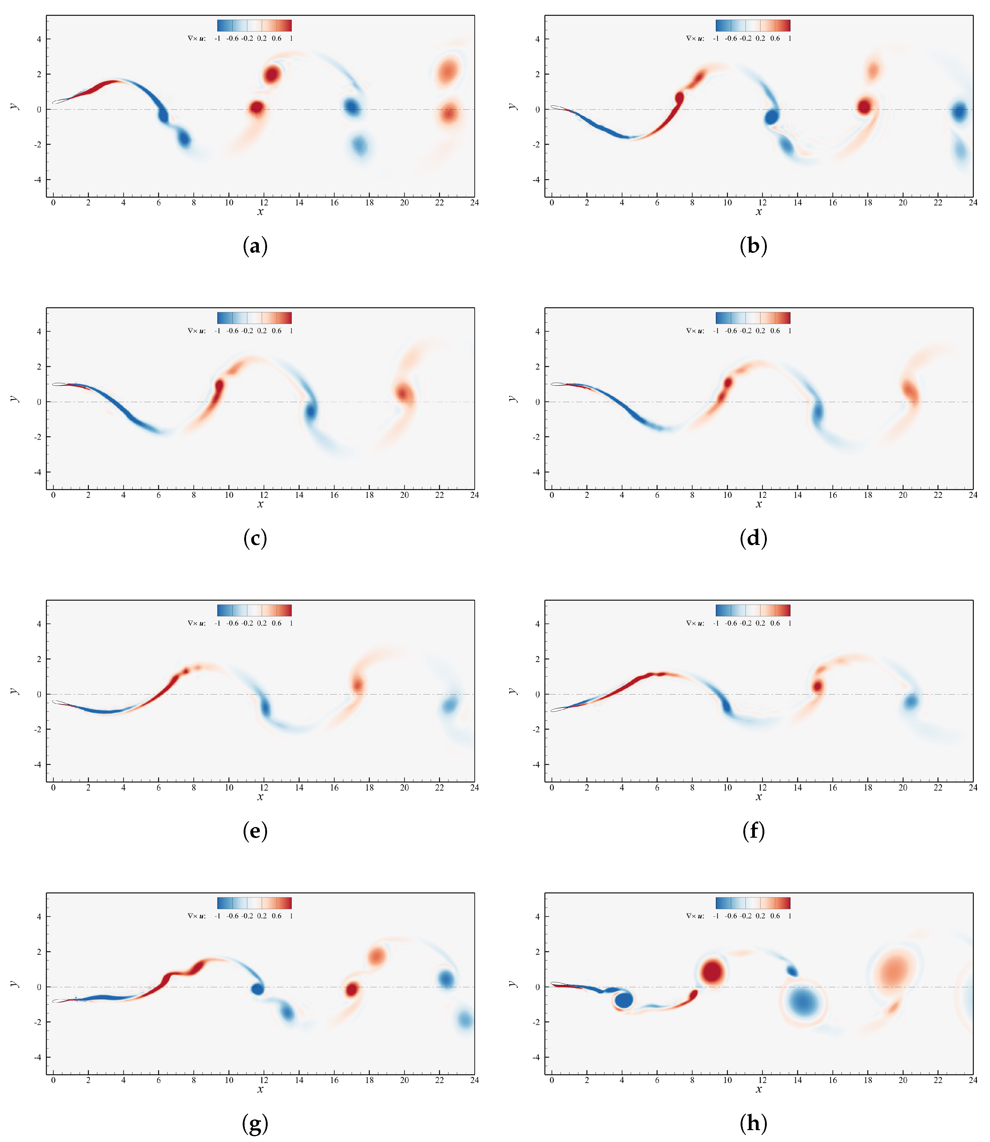
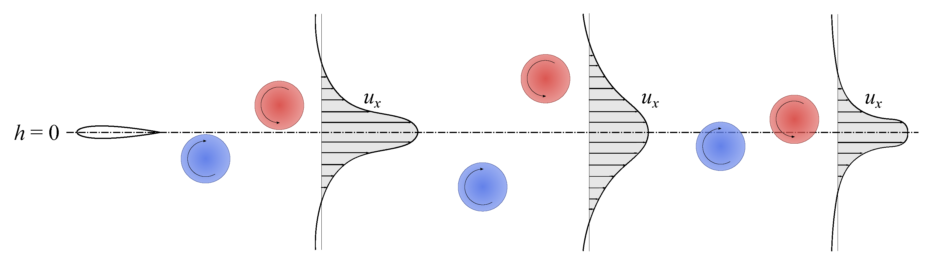
Figure 8 displays how the vorticity field is affected by the phase shift variation. In the interval considered, the flows past the foil are almost identical when
and this finds confirmation in their very similar propulsive performance. The wake topology, in particular, tends to a 2S reverse von Kármán. The only visible difference among the various cases is the width of the wake, which decreases as
increases. This could justify the highest efficiency at
through the observation that the single vortices shed each half cycle are closer to the neutral axis. Indeed, as long as the counterclockwise vortices are above
and the clockwise vortices are below it, the propelling action is more effective if the eddies are close to the neutral position, since the velocity distributes as a concentrated jet. A schematic representation of this mechanism is illustrated in
Figure 13. Outside of the interval
the wake becomes 2P, although starting from
it tends to go back to a 2S pattern. Specifically, the change in slope of
at
in
Figure 5 may be associated to the detrimental vortices
which move upward and vertically align with the eddies
. Their alignment causes their contributions to forward motion to cancel out, leading to little neat thrust. Once
the vortices
almost vanish, however
are squeezed towards the centerline and their contribution starts to cancel out, as discussed right before.
5. Conclusions
Several simulations involving the dynamics of a flapping NACA0015 profile were performed on top a discontinuous Galerkin solver, where the high-order numerical framework was exploited to ensure the resolution independence of the output data.
A wide range of kinematic configurations was presented, involving multiple heaving amplitudes, Strouhal numbers, pitch and phase angles, so to replicate the typical operational conditions of BCF swimmers. A detailed analysis of the problem sensitivity upon such variables was performed, and original observations concerning the relevance of dynamic stall and phase shift effects were advanced.
The results highlighted that, when employing thrusters with an imposed kinematics that makes use of circulatory-based propulsion mechanisms, the most relevant features influencing the propulsive performance appear to be the angle of attack and its rate of change. Upon inspection of the maximum angles of attack in the space of the tested configurations, the presence of a global optimum from an efficiency standpoint clearly emerged, located in the range . The display of a localized peak at such values well above static stall, and the retaining of considerably high efficiency values for even larger , might be traced back to a leading edge separation delay imposed by the unsteady motion effects, associated to the sinusoidal . Furthermore, considering simple balance equations it was showed, for circulatory-dominated propulsion, the necessity of constraining the operational conditions within a regime ensuring high lift-to-drag ratios, so to guarantee high propulsive efficiency.
As far as pitch angle is concerned, the explored configurations manifested an optimal efficiency for , corresponding to the interval in which the lift-to-drag ratio of the profile is maximized. Furthermore, the inspection of the spanwise vorticity fields underlined the influence of the pitch amplitude on the vorticity pattern arising behind the profile. Specifically, vortices seems to be formed at two distinct separation stages, namely once the maximum instantaneous angle of attack is reached and when rate of change of assumes the highest value.
Concerning the effects of Strouhal number and heave amplitude, it emerged once again the key role played by the dynamics of . For fixed and , a given Strouhal number directly sets , while directly modulates the frequency of the motion cycle. Optimal efficiency was found in the interval , while mean thrust coefficient increases monotonically up to , in line with the majority of the works published on the subject. For values of well above the static stall condition, large heave amplitudes, i.e. high frequencies, emerged as a feasible strategy to get very high efficiency. Such condition, indeed, results in an increase of which allows to postpone leading edge separation and maintain significant lift production at large angles of attack. On the other hand, when the maximum angle of attack reached during the oscillating period is smaller than the static stall value, an efficiency improvement was observed for narrow heave amplitudes. For such cases the low frequency also brought to a decrease of the hysteresis in the plane.
A similar behavior in terms of hysteresis reduction was also detected when examining the performance sensitivity to the phase shift. From a dynamic viewpoint, the reduction of the loads hysteresis cycle appears to have the function of compensating the dynamic effects owed to the profile motion. An adequate choice of , in particular, allows for a faster inversion of the lift sign in the transition between upstroke and downstroke, limiting the portion of the cycle where the profile might have a detrimental propulsive behavior. The results showed an optimal efficiency for , which in literature is typically identified at .


