Article

Analyzing Pile-Up Crash Severity: Insights from Real-Time Traffic and Environmental Factors Using Ensemble Machine Learning and Shapley Additive Explanations Method

by
Seyed Alireza Samerei
1,
Kayvan Aghabayk
1,* and
Alfonso Montella
2
1
School of Civil Engineering, College of Engineering, University of Tehran, Tehran 4563-11155, Iran
2
Department of Civil, Architectural and Environmental Engineering, University of Naples Federico II, 80125 Naples, Italy
*
Author to whom correspondence should be addressed.
Safety 2024, 10(1), 22; https://doi.org/10.3390/safety10010022
Submission received: 31 December 2023 / Revised: 12 February 2024 / Accepted: 19 February 2024 / Published: 23 February 2024

Abstract

:
Pile-up (PU) crashes, which involve multiple collisions between more than two vehicles within a brief timeframe, carry substantial consequences, including fatalities and significant damages. This study aims to investigate the real-time traffic, environmental, and crash characteristics and their interactions in terms of their contributions to severe PU crashes, which have been understudied. This study investigates and interprets the effects of Total Volume/Capacity (TV/C), “Heavy Vehicles Volume/Total Volume” (HVV/TV), and average speed. For this purpose, the PU crash severity was modelled and interpreted using the crash and real-time traffic data of Iran’s freeways over a 5-year period. Among six machine learning methods, the CatBoost model demonstrated superior performance, interpreted via the SHAP method. The results indicate that avg.speed > 90 km/h, TV/C < 0.6, HVV/TV ≥ 0.1, horizontal curves, longitudinal grades, nighttime, and the involvement of heavy vehicles are associated with the risk of severe PU crashes. Additionally, several interactions are associated with severe PU crashes, including the co-occurrence of TV/C ≈ 0.1, HVV/TV ≥ 0.25, and nighttime; the interactions between TV/C ≈ 0.1 or 0.45, HVV/TV ≥ 0.25, and avg.speed > 90 km/h; horizontal curves and high average speeds; horizontal curves; and nighttime. Overall, this research provides essential insights into traffic and environmental factors driving severe PU crashes, supporting informed decision-making for policymakers.

1. Introduction

Despite the extensive efforts of transportation organizations worldwide to reduce the frequency and severity of road crashes through road design improvements, vehicle technology, transportation policies, and emergency services, road crashes still remain a major cause of financial and life losses [1]. According to the World Health Organization [2], road crashes result in 1.19 million deaths and between 20 and 50 million injuries annually, with a notable rise in traffic-related fatalities reported in low-income countries, mostly due to the rapid expansion of motor vehicle usage in developing nations. Iran, as a developing country, has one of the highest rates of traffic-related fatalities, with a rate of 15.6 fatalities per 100,000 people [3,4]. In Iranian suburban freeways, the recorded number of crashes in the 5-year period from March 2014 to March 2019 was 51,032, of which 2165 were PU crashes, involving three or more vehicles in a single collision and causing 105 fatalities and 516 injuries. PU crashes have significant consequences such as a high risk of fatalities and injuries, traffic congestion, liability lawsuits, and criminal charges against the at-fault drivers, which are not easily discernible. A considerable amount of social and economic capital is preserved by eliminating these types of collisions. Therefore, it is necessary to outline the definition of a PU crash, the potential risk factors, and the analysis tools which are discussed in the following sections.

1.1. Definition and Background of PU Crash

The mechanism of crashes varies based on the number of vehicles involved [5], including single-vehicle (SV) and multi-vehicle (MV) crashes, which are usually investigated separately due to their different mechanisms and suitable countermeasures [6,7,8,9]. PU crashes, also referred to as chain-reaction crashes, occur when three or more vehicles are involved in a series of successive collisions with each other in a short period of time, making them a distinct type of multi-vehicle (MV) crash. This type of crash is distinct from secondary crashes and consecutive crashes, which involve a set of multiple influential crashes occurring within a specific time interval [10]. According to previous studies, PU crashes occur due to sudden maneuvers of the leading vehicle (e.g., abrupt speed reduction or lane change) [11]. Additionally, simulation results of car-following models have shown that traffic conditions (speed and relative speed) and driver reaction speed significantly affect the occurrence of PU crashes [12].
To the best of our knowledge, no study has specifically examined PU crash severity. However, due to the similarities in the mechanisms of occurrence between secondary crashes, consecutive crashes, and PU crashes, the background literature of secondary crashes and consecutive crashes has been investigated in this study. Most studies have focused on the probability of secondary and consecutive crashes, as comprehensively discussed in [10,13]. These studies mainly discuss the implications of delays and service level reduction resulting from these crashes, with limited examination of the severity of secondary and consecutive crashes. Meng et al. [5] examined the severity of consecutive crashes from the perspective of exploring the relationship between a set of closely occurring crashes. The findings indicated that the type of primary crash has an impact on the severity of secondary crashes, and speed limits, traffic volume, and adverse weather conditions increase the severity of consecutive crashes. According to Li et al. [14], although secondary crashes constitute a relatively small portion of road crashes compared to regular crashes, they have the potential of causing more injuries and fatalities. Also, they indicate that occupancy, time gap between two crashes, number of lane changes, and the number of lanes is associated with the severity of secondary crashes. Huang et al. [15] investigated the crash severities by simultaneously modeling primary crashes and secondary crashes and examining how traffic changes resulting from primary crashes affect the severity of secondary crashes. According to their results, speed variations and traffic conditions resulting from a primary crash have an impact on the severity of secondary crashes.

1.2. Importance of Real-Time Traffic Characteristics in Safety

Given the significant impact of traffic parameters on safety and the potential for managing them to improve safety outcomes, researchers have consistently emphasized the importance of incorporating traffic variables in safety studies. In most previous studies, static and aggregated traffic measures, such as AADT or monthly traffic volume, and speed limits have been used to model the occurrence of secondary crashes [10,16,17]. However, these measures do not precisely reflect the traffic conditions immediately before the occurrence of crashes and may lead to biased results [18]. Recent studies have emphasized the investigation of the impact of traffic dynamics (traffic changes resulting from primary crashes) on the severity of secondary crashes and the probability of their occurrence [14,15,19,20]. Additionally, considering real-time traffic characteristics enables the identification of more accurate traffic situations leading to secondary crashes [13,21]. Other studies examining crash severity (regardless of the specific type of collision), such as [22], have also pointed out the influence of real-time traffic on crash severity, while [23] examined the impact of AADT and average speed on crash severity as well.
For two routes with equal traffic flow, different capacity will lead to different traffic conditions. Thus, it is appropriate to consider the Total Volume/Capacity (TV/C) ratio, which indicates the degree of saturation or congestion on the route [18,24]. In most studies, less-congested conditions have been introduced as a contributory factor to serious crashes due to high speed. However, some inconsistent results related to the effects of congestion on road safety cause confusion for transport planners and safety policymakers. For instance, Quddus et al. [25] point out that congestion is not related to crash severity, yet according to Wang et al. [26], increases in congestion are associated with the risk of severe crashes. Therefore, a solely qualitative description of traffic and congestion conditions will not be informative and the critical values of congestion should be extracted and interpreted. In addition, previous studies on crash severity have paid limited attention to the impact of heavy vehicles, such as trucks and buses, in traffic composition. Due to the size, weight, and potential unsafe interactions of trucks with other vehicles, neglecting their ratio in traffic combination may lead to biased results.

1.3. Application of Machine Learning and Interpretation Methods

In recent decades, numerous studies and modeling efforts have been conducted in the fields of safety and crash severity, focusing on crash data and predominantly using Statistical Methods (SMs). Statistical modeling requires assumptions about the distribution of data, which may be violated, leading to incorrect estimates and erroneous inferences. Machine learning (ML) methods have shown increasing growth in safety analysis in recent years [27,28]. These methods involve processes for identifying hidden structures, associations, and patterns [29,30,31,32,33,34,35,36]. These techniques utilize complex structures and algorithms to understand patterns and relationships between input and output data, typically outperforming statistical models in comparative studies [37,38,39,40].
Considering the complexity of PU crashes and the interaction of factors, a method capable of modeling complex patterns is needed. ML can handle large and complex datasets, provide relatively short computational modeling time, and offer satisfactory accuracy [41]. In recent years, ML techniques have been used for predicting and modeling crash severity [42]. The most well-known models utilized in safety and crash modeling studies are gradient-boosting decision tree models, such as XGBoost [43,44,45], CatBoost [46], AdaBoost [43], and LightGBM [47].
Regardless of the accuracy of the ML models, the interpretability of the model results plays a crucial role. Decision- and policy-making is possible only through fully understanding the model and properly interpreting its results, and interpretability in ML is of particular importance for generating reliable models [48]. Due to the complex structures of many ML models (often referred to as “black-box” models), interpreting the results of these models poses challenges [38]. In previous safety studies, several post hoc analyses have been used to interpret the results of models. The Local Sensitivity Analysis (LSA) method has been employed in some studies to calculate sensitivity analysis and elasticity analysis in crash severity modeling. In these analyses, all variables are held constant except for the variable of interest, and the changes in the model’s results are recorded as a percentage of variation [49,50,51]. Partial Dependence Plots (PDPs) are one of the most common methods used to interpret the results of ML models in safety studies. PDPs show the effect of all values of a feature on predicting the dependent variable based on the marginal distributions of other variables [52]. PDPs have been utilized to interpret the results of ML models in safety studies [53]. However, PDPs have the limiting assumption of uncorrelated input variables, which is considered a fundamental constraint and can lead to biased results [27,54,55]. To address this issue, the Shapley Additive exPlanations (SHAP) method, which has the capability to estimate the effects of variables and their interactions on the output, was introduced in [56]. SHAP analysis has been employed in recent safety studies, including factors affecting the occurrence of crashes [57,58] and crash severity [43,44].

1.4. Aims

Considering the unique mechanisms, involvement of numerous vehicles, and severe consequences leading to the high fatality and injury rates of PU crashes, obtaining a precise understanding of the influencing factors is significant. Thus, this research aims to investigate the factors influencing PU crash severity, particularly focusing on the gaps in environmental conditions and real-time traffic interactions. Recognizing the crucial role of the traffic conditions, this study utilizes real-time TV/C for a more accurate assessment, instead of relying on aggregated data like the AADT. Given the inconsistent results of previous studies regarding the effects of TV/C, there is a need to investigate critical TV/C values and interpret their impact on PU crash severity. Additionally, while previous research has examined heavy vehicle involvement in crashes, there has been limited exploration of the proportion of heavy vehicle traffic and its relative effects on crash severity. Moreover, by employing ML models and the SHAP method, this research delves into the involvement and interactions of multiple factors in PU crashes, enhancing understanding and interpretation of the results for a broad audience of transport planners and safety policymakers. The use of SHAP provides probability plots, highlighting critical values for better decision-making. Therefore, the primary goals of this study encompass the following:
  • Exploring the interacting effects of real-time traffic parameters and environmental conditions on the severity of PU crashes to address these rare and complex aspects of traffic incidents.
  • Utilizing ML models and the SHAP method, proficient in identifying complex patterns and interpreting influence and interactions, in order to present results that are easily interpretable for policymakers.
The rest of the article is organized as follows. First, in Section 2, the source and characteristics of data and their initial analysis are presented. In Section 3, the details of the ML methods and SHAP analysis are reviewed. In Section 4, the outputs and results of modeling are interpreted and discussed. Section 5 provides the summary and conclusion, while limitations and future directions are discussed in Section 6.

2. Data

The data used in this study pertain to 2165 PU crashes that occurred on eleven major suburban freeways in Iran with a total length of 2015 km, including 255 sections, as shown in Figure 1. In all freeways considered in this study, the speed limit is set at 120 km/h for passenger cars and 110 km/h for heavy vehicles, and there are two to three lanes for each direction. The data used in this study consist of PU crash data that occurred over a 5-year period (March 2014 to March 2019), collected by the police at the crash scenes and encompassing environmental and crash characteristics. Additionally, to examine the impact of real-time traffic variables, including the traffic volume of different types of vehicles, capacity of each segment, and average vehicle speed, data obtained from the Iran Road Maintenance and Transportation Organization were utilized [59]. The traffic data in this study are based on the recorded data from loop detectors along the routes. After assessing different time intervals for aggregating traffic data, the 1 h period before a crash better distinguished the overall traffic conditions between severe PU crashes and non-severe PU crashes in terms of model performance and practicality. Hence, in this study, a mesoscopic analysis approach was pursued, which has also been employed in [25,60]. Based on the location of each crash and the time of crash occurrence, the 1 h pre-crash real-time traffic information recorded by the upstream loop detector was aggregated and matched with the respective crash. Further details regarding the traffic data, PU crash characteristics, and environmental parameters will be explained in subsequent sections.
According to previous studies, the PU crashes in this study have two conditions: 1—more than two vehicles colliding directly with each other within a limited time period, and 2—no other crash occurred within a 2 h time interval before and after the PU crashes, indicating that a PU crash is neither a cause of crashes (primary), nor the result of a crash (secondary). According to the PU crash data, 19.3% of crashes resulted in fatality and injury (F&IN) at the crash scene and 80.7% of crashes resulted in property damage only (PDO). Table 1 presents the descriptive statistics of the variables related to crashes. More details about the data are given in the next sub-sections.

2.1. Real-Time Traffic Characteristics

Based on the capacity of each road segment and the traffic volume before the occurrence of PU crashes, for each crash, the ratio of T o t a l   V o l u m e / C a p a c i t y   ( T V / C ) was evaluated. The capacity data for each freeway segment in our study were obtained from [59], and capacity adjustments were implemented for sections where PU crashes occurred in rain, snow, and fog, with reference to the Highway Capacity Manual. T V / C indicates the degree of saturation and its examination has been emphasized for crash severity modelling [61]. The ratio of heavy vehicles in the traffic combination prior to a crash event is another potential factor that could impact the severity of the collision. This ratio, labeled as H e a v y   V e h i c l e s   V o l . / T o t a l   V o l .   ( H V V / T V ) , was matched with each crash based on the date and time of the crash. In most previous studies, only the speed limit of the segment was considered as a parameter, and the speed limit on all freeways in Iran is 120 km/h for passenger cars and 110 km/h for heavy vehicles, which does not provide useful information about traffic conditions. According to [62], the relationship between speed and road safety is consistent at both the individual driver level and the aggregate level (average traffic speed). Therefore, in this study, the average speed of vehicles at the upstream location of the PU crashes was extracted and matched with each information row of PU crashes.
To understand the underlying distribution of real-time traffic variables related to PU crashes and comparing their distributions in two levels of severity (PDO and F&IN), kernel density plots were drawn (Figure 2). A kernel density plot is an extended version of a histogram that uses a kernel function to smooth out the frequency bins. It estimates a probability density function that provides a more accurate representation of the distribution and concentration of the target variable. Based on Figure 2a, F&IN crashes have the highest concentration of about T V / C 0.1 , while PDO crashes are concentrated in two ranges of T V / C 0.2 and T V / C 0.8 . According to Figure 2b, the peak of PDO crashes is located at H V V / T V 0.1 and is more concentrated in lower H V V / T V values compared to the F&IN distribution. On the other hand, the peak of F&IN crashes is H V V / T V 0.15 and has a higher probability than PDO crashes for higher H V V / T V values. Figure 2c displays the distribution of the average speeds of passing vehicles before PU crashes. The distribution of average speeds for F&IN crashes is concentrated around 105 km/h, while for PDO crashes, it is in the range of 85 km/h.
Considering the likelihood of correlation between traffic variables and a better understanding of incorporating these parameters into the main model, a Matrix Scatter plot was drawn for these variables (Figure 3). As expected, the average speed generally showed a negative correlation with T V / C , and in T V / C > 0.6 , the average speed noticeably decreased. In the range of T V / C < 0.6 (green rectangle), especially in the less-congested traffic range where F&IN crashes are mostly located, no significant correlation is observed. It seems that in non-congested traffic ( 0.0 < T V / C < 0.2 ), although driving at speeds higher than 120 km/h is possible, drivers are still required to adhere to speed limits. However, in less-congested traffic ( 0.2 < T V / C < 0.4 ), where speed reduction is practically necessary, most drivers prefer to drive at the maximum permissible speed. Additionally, in non-congested traffic ( 0.0 < T V / C < 0.2 ) with a high percentage of heavy vehicles ( 0.3 < H V V / T V < 0.6 ), the average speed of the segment is lower compared to cases where passenger cars form most of the traffic composition. Therefore, it is valuable to investigate the interaction between average speed and T V / C in light traffic conditions and their impact on PU crash severity.
Typically, the traffic volume of heavy vehicles such as trucks and buses remains relatively stable on most routes. However, during certain occasions such as extended holidays, there may be an increase in demand for passenger car travel, while restrictions on some truck traffic may be in place. Therefore, the traffic rate of passenger cars mostly determines the traffic composition. As expected, when there is an increase in demand for passenger car travel and heavy traffic occurs ( T V / C > 0.6 ), the H V V / T V ratio tends to decrease (Figure 3). However, as noted within the shaded area in dark red, the opposite scenario does not hold true. In other words, in conditions where T V / C < 0.6 , which include a high number of F&IN crashes, a high H V V / T V ratio is not necessarily present, and a correlation between T V / C and H V V / T V is not apparent.

2.2. Crash Characteristics

The primary distinction between PU crashes and other types of collisions is the number of vehicles involved in a single crash. The PU crashes examined in this research involved 3 to 12 vehicles. Crashes involving more than five vehicles were categorized in one group. The frequency of PU crashes by the number of involved vehicles is shown in Figure 4a (to enhance the graph’s visual display, the percentage of each subgroup is represented). While most crashes (81.8%) involve three vehicles, the rate of F&IN crashes dramatically increases with the number of involved vehicles. This trend also holds for the number of heavy vehicles involved in PU crashes, as shown in Figure 4b.
The high rate of F&IN in PU crashes with many vehicles involved and the relatively low number of these critical events compared to PU crashes with three vehicles involved leads to biased modeling of crash severity and the underestimation of the importance of these types of PU crashes. Therefore, to address the imbalance in PU crash data in terms of the number of vehicles involved, data resampling was performed, and the method and corresponding results are presented in the Methodology and Results and Discussion Sections.
Due to the larger size of trucks, trailer trucks, and buses compared to passenger cars, and their impact on driving conditions and the surrounding vehicles, they may create hazardous conditions. Moreover, their higher weight may lead to severe collisions. By aggregating these vehicles into the heavy vehicle variable in this study, their impact on traffic composition and their involvement in PU crashes are investigated.

2.3. Environmental Factors

One of the environmental variables of this study is the road geometry, which is divided into four categories: curve and longitudinal slope, curve and plain, straight and longitudinal slope, and straight and plain. Also, the road lighting status is divided into Day, Night, Sunrise, and Sunset categories based on the time. There is information about weather conditions (cloudy and foggy and dusty, rainy, smooth, snow, storm) and road surface conditions (dry, wet, ice, and snow) in the crash database, where only the road surface condition variable was used in modeling due to high correlation. The variables of the number of crossing lanes and land use were also used in this study.

3. Methodology

We used and compared six tree-based and ensemble ML models: Classification and Regression Trees (CART), Random Forest (RF) [63], Extreme Gradient Boosting (XGBoost) [64], Categorical Boosting (CatBoost) [65], Light Gradient Boosting Machine (LightGBM) [66], and Adaptive Boosting (AdaBoost) [67]. The CART model, also known as a decision tree, has a tree-like structure consisting of a root node (topmost node), internal nodes, and leaf nodes (end nodes). Decision tree algorithms usually proceed from top to bottom, selecting a splitter at each stage that provides the best split, and continue growing until the dataset is divided into groups that are as homogeneous and consistent as possible.
The RF model creates multiple decision trees and combines their results, known as an ensemble ML technique. To construct this predictive tool, sampling with replacement is first performed on the data with equal size. In the next step, a classification model (decision tree) is built for each sample. Each tree votes for the most popular class/category. Finally, the majority vote is considered the output.
Gradient Boosting is an ML technique used for regression and classification problems, introduced as Gradient-Boosted Machines by Friedman in 2001. Typically, in this technique, decision trees (usually CART) with a fixed size are used as base learners, and the boosted trees are called gradient-boosting decision trees (GBDT). Unlike RF, which is composed of independent trees, the GBDT model sequentially creates a set of shallow and weak trees. Each new tree in GBDT improves the previous trained tree by applying higher weights to misclassified observations and lower weights to correctly classified observations. When weak trees are boosted, the probability of correct classification for observations with high weight increases. Therefore, the GBDT model transforms a set of weak learners into a strong model and predicts challenging classification cases. The other models mentioned in this study are considered subsets of GBDT, which have been enhanced in various aspects. Next, only the CatBoost model, which had the best performance in this study, is described. The subsequent sections of this part explain the details of resampling, hyperparameter tuning, model evaluation, and model interpretation in order.

3.1. Categorical Boosting Method (CatBoost)

The CatBoost is a novel version of the Gradient-Boosting Decision Tree algorithm. The Gradient-Boosting Decision Tree (GBDT) algorithm combines numerous decision trees to create a high-accuracy model, and the process can be expressed as Equation (1):
y x = t = 1 T f t x , θ t  
where x denotes the variable vector, T denotes the number of trees, θ t t = 1,2 , , T denotes a learned parameter, and f t x , θ t denotes the learned decision trees that are learned. Given a set of training samples D = x k , y k 1 n , where n denotes the total number of samples in training data, x k k = 1,2 , , n is the sample data points, and y k indicates the true sample label. In order to learn the model in Equation (1), Equation (2)’s objective function is required to be minimized:
O f t = i = 1 n L y k , y k   + t = 1 T Ω f t  
where y k denotes the predicted sample label, L represents the loss function, which is actually the difference between y k and y k , and Ω represents the regular function, which is employed to penalize the complexity of f t . It is defined as Equation (3):
Ω = α q + 1 2 β ω 2
where α denotes a penalty parameter, which controls the number of leaf nodes q , β represents the regularization parameter, and ω represents the weight coefficient. Let ζ represent the loss function negative gradient, then the objective function is minimized in the direction of ζ given by Equation (4):
ζ = L y k , y ¯ k y ¯ k
The CatBoost algorithm differs from the other GBTs in terms of having two prominent features, i.e., efficient handling of categorical features and ordered boosting [68]. The learning classifiers handle numerical features quite efficiently during the model training phase; however, interpreting categorical features is complicated for them. Therefore, in conventional approaches, categorical features are transformed into useful information using the one-hot encoding technique or gradient statistics. In the former technique, each category of the original categorical features is replaced by the binary values, while in the latter technique, an estimated value is generated by using gradient statistics to replace the original categorical feature at each boosting step. Nevertheless, in the case of the categorical features with high repeatability, both the mentioned techniques require large memory and other computational resources. To avoid the mentioned problem, the CatBoost algorithm utilizes efficient modified target-based statistics to appropriately handle the categorical features during training time, thus saving considerable computational time and resources. Another important aspect of the CatBoost algorithm is its ordered boosting mechanism. In traditional GBTs, all the training samples are provided to construct a prediction model after executing several boosting steps. This approach causes a prediction shift in the constructed model, which consequently leads to a special kind of target leakage problem. The CatBoost algorithm avoids the stated issue by utilizing the ordered boosting framework. Furthermore, contrary to the conventional learning classifiers, the CatBoost algorithm eloquently handles the overfitting issue by using several permutations of the training dataset [69]. The strategy for optimizing greedy target-based statistics is expressed in Equation (5):
x k i ¯ = j = 1 n x j i = x k i y i + a P     j = 1 n x j i = x k i + a    
where x k i denotes the k th sample’s i th category variable, x k i ¯ denotes the corresponding variable, P denotes the increased prior value, and a denotes the weight coefficient a > 0 . Prior values can be used to effectively reduce noise introduced by low-frequency variables and avoid the overfitting phenomenon [43].

3.2. Resampling

The PU crash data are highly imbalanced based on the number of vehicles involved, as shown in Figure 4. Consequently, crashes with a high number of vehicles involved that have higher rates of F&IN might be less considered and lead to bias in modelling. To address this issue, oversampling can be used, which not only addresses the imbalance in the PU crash data, but also alleviates the imbalance in the severity levels. In this study, the random oversampling method was used, which resulted in improved accuracy in predicting the crash type [70]. This method randomly selects the samples from the minority class, with replacement, and adds them to the training dataset.

3.3. Hyperparameter Tuning

Hyperparameter tuning is a critical aspect of machine learning, aimed at identifying the optimal set of hyperparameters for a model. This approach is instrumental in preventing the development of an overfitted and excessively complex model [47,71]. In this study, the GridSearch technique is employed to discover the best combination of hyperparameters utilizing 10-fold cross validation and the ROC-AUC of the model is collected as a performance metric.

3.4. Model Evaluation

The performance of ML models can be evaluated by a number of metrics, which can be generally derived from the model’s confusion matrix shown in Table 2.
To assess the model’s performance using the classification table, the following measurements should be calculated first:
A c c u r a c y = T P + T N ) / ( P + N
P r e c i s i o n = T P / ( T P + F P )
R e c a l l   o r   T P R = T P / ( T P + F N )
F P R = F P ( F P + T N )
F 1 s c o r e = 2 × P r e c i s i o n × R e c a l l P r e c i s i o n + R e c a l l
Equation (6) can be used to obtain the model’s overall accuracy. The closer the model is to 1 in accuracy, the stronger it is at classifying the samples. Equation (7) indicates the ratio of correctly predicted positive observations to the total predicted positive observations, which shows the accuracy of the model. Also, high precision relates to low FPs. Equation (8) represents the ratio of correctly predicted positive observations to all observations in the actual class, which shows the sensitivity of the model, and low Recall indicates the presence of a large number of FNs. The TPR quantifies the proportion of positives correctly identified, whereas the FPR quantifies the proportion of negatives incorrectly classified as positives. This metric could lead to specious results with unbalanced data sets. To address this issue, F1 Score (Equation (9)) might be a better measure to use if we need to seek a balance between Precision and Recall. To gain a better understanding of how well a model performed, an area under the receiver operating characteristic (AUC-ROC) curve was also used. The ROC curve was obtained by plotting the FPR on the x-axis and TPR on the y-axis. The two-dimensional area underneath the entire ROC curve is called the area under the ROC curve and the AUC values range from 0 (completely incorrect) to 1 (perfectly correct).

3.5. Model Interpretation

SHAP is a novel model interpretation method for explaining the output of an ML model by assigning importance values to each feature in a prediction [56]. The SHAP value is based on the concept of Shapley values from cooperative game theory [72], which assigns a value to each player in a game based on their marginal contribution to the game outcome when playing in a coalition with other players. The SHAP value of a feature represents the contribution of that feature to the predicted outcome compared to the average prediction across all possible feature combinations. To compute the SHAP value of a feature, the SHAP algorithm considers all possible feature combinations and calculates the difference in prediction between the current feature set and the feature set with the feature removed. This difference is then averaged over all possible feature combinations, giving the SHAP value for that feature. The SHAP values can be used to explain individual predictions by showing the contribution of each feature to the prediction, or to provide an overall understanding of the model by analyzing the distribution of SHAP values for all features.
For a risk factor subset S F (where F stands for the set of all risk factors), two models are trained to extract the effects of factor i . The first model f S i x S i is trained with factor i while the other one f S x S is trained without it, where x S i and x S are the values of input features/risk factors. The difference in model outputs f S i x S i f S x S is computed for each possible subset S F i . The Shapley value of a risk factor i is calculated using Equation (11):
i = S F i S ! F S 1 ! F !   f i x S i f S x S
Local SHAP values refer to the effects of risk factors calculated based on one observation, while global SHAP values represent the importance of risk factors and the interaction effects of two factors based on all observations. For example, the SHAP interaction values can be calculated as the difference between the Shapley values of factor i with and without factor j in Equation (12) [47]:
i , j = S F { { i , j }   | S | ! ( | F | | S | 2 ) ! | F | ! f S { i , j } x S { i , j } f S { i } x S { i } f S { j } x S { j } + f S x S
In this study, the Shapley values were computed using a recently introduced technique called tree-SHAP developed by [73]. The tree-SHAP algorithm is specially designed for tree-based models, and ensemble gradient-boosted machines. One of the important features of this algorithm is that it computes the local feature interaction, which in turn facilitates the interpretation of the global model structure for each prediction. The analysis was performed under the Python 3.8 environment and ML and SHAP packages were used for model training, evaluation, and interpretation.

4. Results and Discussion

4.1. Model Fitting and Evaluation Results

Considering the imbalance PU crash data and the likelihood of model bias towards crashes with a high number of vehicles involved, resampling improves the accuracy of the models. In the first step, the minority classes in the PU crash data were resampled using the random oversampling method, and their distribution is shown in Figure 5. Additionally, to prevent overfitting and model complexity and to increase prediction accuracy, the model hyperparameters should be tuned. Based on the descriptions provided in the Methodology Section and using the variables defined in the Data Section (70% for training data and 30% for testing data), the CART, RF, CatBoost, XGBoost, LightGBM, and AdaBoost models were executed. To compare and evaluate the accuracy and performance of the models, metrics such as accuracy, Recall, Precision, F1 Score, and ROC-AUC were used on the test data. According to the results presented in Table 3, the CatBoost model performed the best. Also, the optimal CatBoost hyperparameter values selected based on the AUC metric were as follows: number of iterations: 500, max depth: 6, ‘l2_leaf_reg’: 1 × 10⁻²⁰, ‘leaf_estimation iterations’: 10, ‘logging_level’: ‘Silent’, ‘loss_function’: ‘Logloss’.
In this study, the SHAP method was used to interpret the results obtained from the CatBoost modeling, and the significant variables were analyzed. The results of this analysis are presented in subsequent sections. Initially, an overview of the results and the importance of variables are provided, followed by an examination of how variables affect the predictions and significant interactions between them.

4.2. Importance and Global Interpretation of Risk Factors

Figure 6a represents the order of importance and the average impact of risk factors on PU crash severity, based on Mean SHAP values. In Figure 6a, risk factors are ranked from top to bottom according to their Mean SHAP values. Figure 6b shows the SHAP summary plot, illustrating the overall impact of risk factors on crash severity (the likelihood of F&IN PU crashes). Positive SHAP values indicate a higher risk of F&IN PU crashes, whereas negative values represent lower risk. For continuous variables, the color bar on the right side indicates the value of risk factors (red dots represent higher values, while blue dots represent lower values). The SHAP values of categorical variables are displayed in gray, and their impact will be further examined in the next sections.
Based on the results shown in Figure 6a,b, the most important variable in PU crash severity is road geometry. The next most significant variable is the number of vehicles involved in PU crashes. The SHAP summary plot in Figure 6b shows that an increase in the number of vehicles involved associated with higher SHAP values and higher probability of F&IN crashes. High average speed is associated with a higher probability of F&IN crashes. Also, T V / C is associated with crash severity. Low values of T V / C lead to the risk of F&IN crashes, and vice versa. The H V V / T V is also influential, and higher values of H V V / T V are associated with an increased probability of F&IN PU crashes. Lighting conditions, road surface conditions, and land use are placed in lower ranks. The next sections will explore the impact and significant interactions of the most important variables on PU crash severity.

4.3. Main and Interacting Effects of Risk Factors

To interpret the impact of each risk variable on PU crash severity, SHAP dependence plots are presented for each significant variable in this section. In each subplot, the horizontal axis represents the values of the independent variable, and the left vertical axis represents the SHAP value (positive SHAP values indicate the positive probability of F&IN PU crashes). In the subplots where independent variable interactions are considered, the right vertical axis represents the secondary independent variable, which is displayed as a color bar.

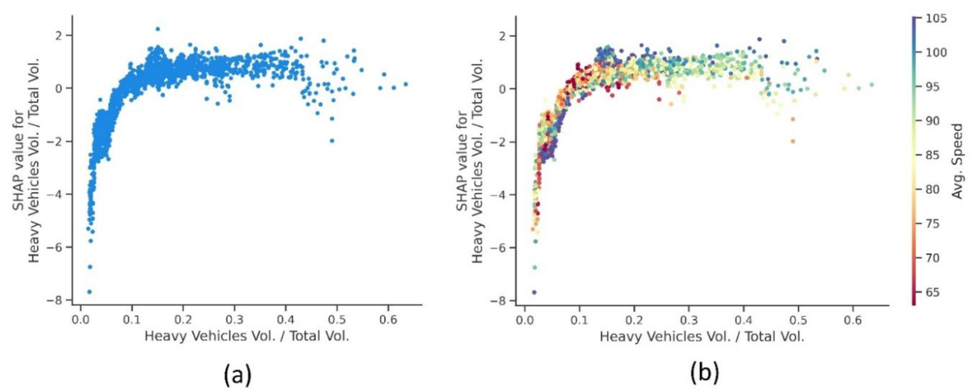
4.3.1. Real-Time Traffic Factors

Figure 7 illustrates the main effects of average speed, T V / C , and H V V / T V . According to the results in Figure 7a, average speeds above 90 km/h are associated with the risk of F&IN crashes, and vice versa. Moreover, the probability of F&IN PU crashes shows an increasing trend with increasing average speed. Studies that have examined speed limits as a parameter have shown that increasing speed limits and the possibility of driving at higher speeds are accompanied by an increase in severe crashes [74,75,76]. It is likely that traffic oscillations at low speeds lead to non-severe crashes [60]. Additionally, significant variations in vehicle speed prior to crashes increase the likelihood of severe crashes [22,23].
According to Figure 7b, T V / C values below 0.6 are associated with a high risk of F&IN PU crashes, while T V / C values above 0.6 are accompanied by a low risk of F&IN PU crashes. The highest positive SHAP value is related to non-congested traffic ( 0.05 T V / C 0.15 ), indicating a higher risk of F&IN severity, and this may be attributed to higher vehicle speeds and driving at free flow speeds. For T V / C 0.1 , the risk of F&IN PU crashes reaches its highest level, which can be considered a critical T V / C condition. Most studies have focused on the impact of traffic flow on the number and risk of crashes. However, according to [77,78,79], the risk of severe crashes is higher in light traffic flow conditions (non-congested traffic) due to relatively high vehicle speeds [62]. Furthermore, with an increase in T V / C , the risk of F&IN PU crashes remains positive but follows a decreasing trend. When T V / C reaches approximately 0.2, the probability of F&IN severity reaches the lowest positive SHAP value. With increased traffic and T V / C 0.45 , the risk of F&IN severity again approaches critical T V / C conditions. In these conditions, the vehicle speed is lower than the free flow speed, but the exposure has increased. According to [26], an increase in congestion is associated with severe crashes, and this may be attributed to higher speed variances between vehicles and lanes, as well as erratic driving behavior that can occur under congested conditions. Also, high traffic flow variations are associated with an increased risk of severe crashes, especially just before congestion formation [22,23,60,61]. Therefore, T V / C 0.45 can be considered a high-risk congestion level, leading to a high risk of severe PU crashes. Furthermore, with an increase in T V / C , the probability of F&IN severity follows a decreasing trend, and at around T V / C 0.6 , the SHAP value reaches zero; thereafter, the risk of F&IN severity decreases, which is primarily due to high congestion and vehicle speed decreasing. In these conditions, with an increase in exposure, the probability of PDO PU crashes increases, resulting in a low risk of F&IN PU crashes [80].
According to the results in Figure 7c, when H V V / T V reaches approximately 0.1, the SHAP value becomes positive and H V V / T V > 0.1 is associated with the risk of severe PU crashes. For H V V / T V > 0.1 , the SHAP value has a positive and steady trend, indicating that the probability of severe F&IN crashes remains positive. Higher values of H V V / T V are mostly related to transit routes where the traffic volume of these vehicles increases, or in other words, the traffic volume of passenger cars decreases. Previous studies mainly focus on truck-involved crashes, and rarely examine the impact of trucks’ presence in traffic on crash severity. However, according to [81], due to the considerable difference in speed between trucks and passenger vehicles, the likelihood of traffic conflicts and collisions increases. Furthermore, [82] found that the interaction between trucks and other vehicles is positively correlated with the risk of other vehicle crashes.
To investigate PU crash severity in greater detail, SHAP dependence plots are presented in Figure 8 and Figure 9, highlighting the main effects and interactions of traffic variables. As T V / C is a crucial indicator of congestion status, Figure 8 illustrates its main effects and significant interactions with other variables. Figure 8a indicates that critical conditions for PU crash severity arise at T V / C values around 0.1 and 0.45. As demonstrated in Figure 8b, higher average speeds within these two risky congestions are associated with higher SHAP values and a higher risk of F&IN PU crashes. Additionally, as shown in Figure 8c, the interaction between T V / C 0.1 and H V V / T V 0.25 leads to high SHAP values. Figure 8d also indicates the high risk of the interaction between T V / C 0.1 and the occurrence of crashes in the darkness of night. It can be inferred that, although the probability of a crash occurrence is lower in non-congested conditions, the risk of severe PU crashes increases under certain conditions. The risk of severe PU crashes increases in specific conditions where T V / C 0.1 , a v g . s p e e d > 90   k m / h, H V V / T V 0.25 , and nighttime darkness interact.
As shown in Figure 9a (or Figure 7c), for HVV/TV ≥ 0.1, it is associated with positive SHAP values and a higher risk of severe F&IN PU crashes. Based on the initial analysis in the Data Section, a high percentage of heavy vehicles are present in light traffic conditions and transit routes, and Figure 8c also demonstrates the positive impact of their interaction on increasing the risk of severe PU crashes. According to Figure 9b, the interaction of H V V / T V 0.10 and a v g . s p e e d > 90   k m / h is associated with higher SHAP values and an increased risk of severe PU crashes.

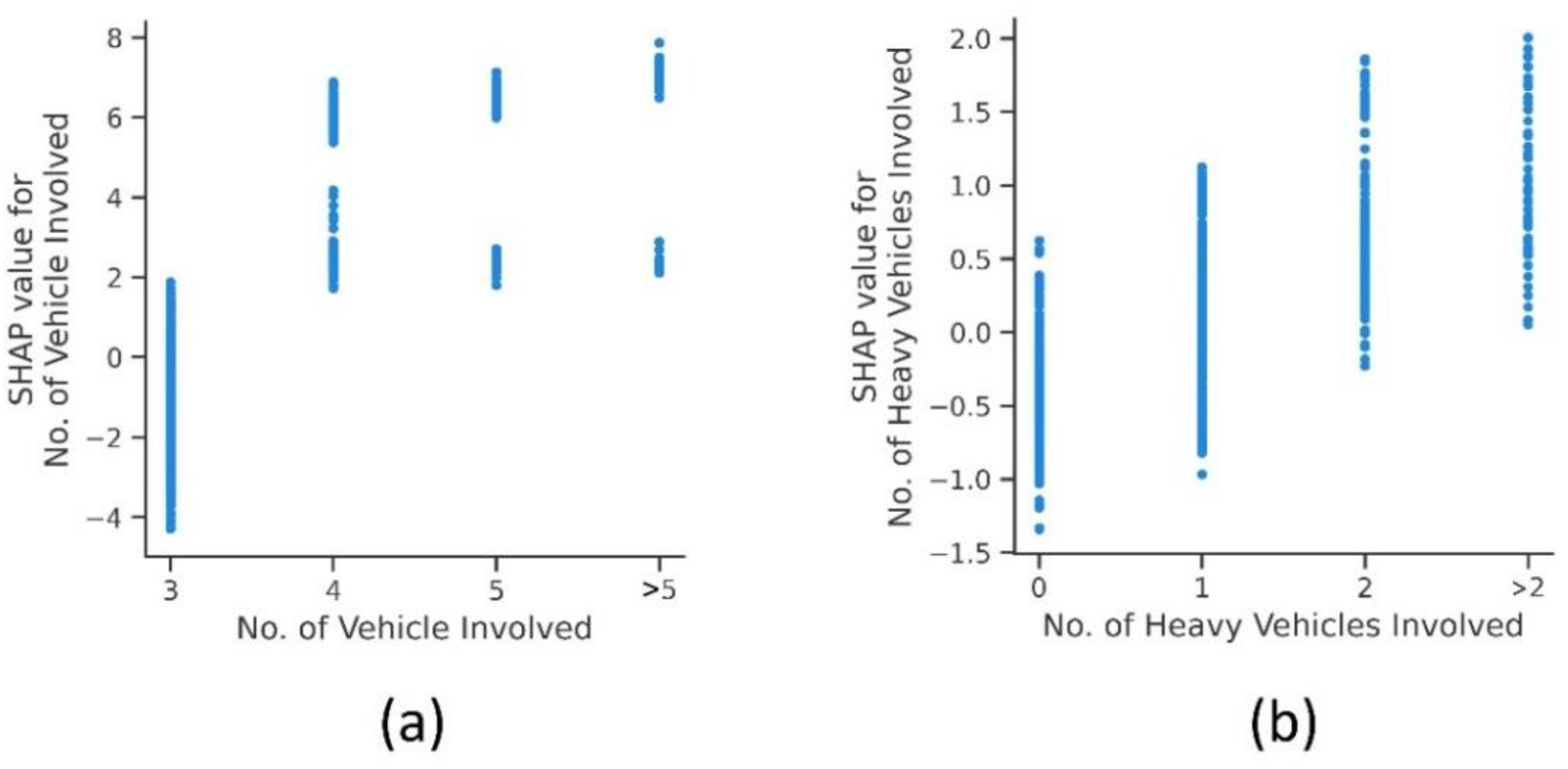
4.3.2. Crash Characteristics

As shown in Figure 10a, the involvement of four or more vehicles in a PU crash is associated with positive SHAP values and higher risk of F&IN PU crashes. As the number of involved vehicles increases, the risk of F&IN PU crashes also increases. As the number of involved vehicles increases, so does the number of impacts and collisions that occur. Initially, the involved vehicles may only suffer minor injuries and damages, but as the collisions continue, the severity of injuries can escalate to more serious injuries or even fatalities. As demonstrated by the SHAP dependence plot in Figure 10b, the collision between a heavy vehicle and other vehicles in PU crashes is associated with positive SHAP values and a higher risk of F&IN PU crashes. An increase in the number of heavy vehicles involved in PU crashes, on average, raises the probability of severe PU crashes. Also, [9,83,84] have also noted that the involvement of large trucks in crashes can lead to severe crash, and this may be attributed to the size and weight of these vehicles, which can result in the release of more energy in collisions.

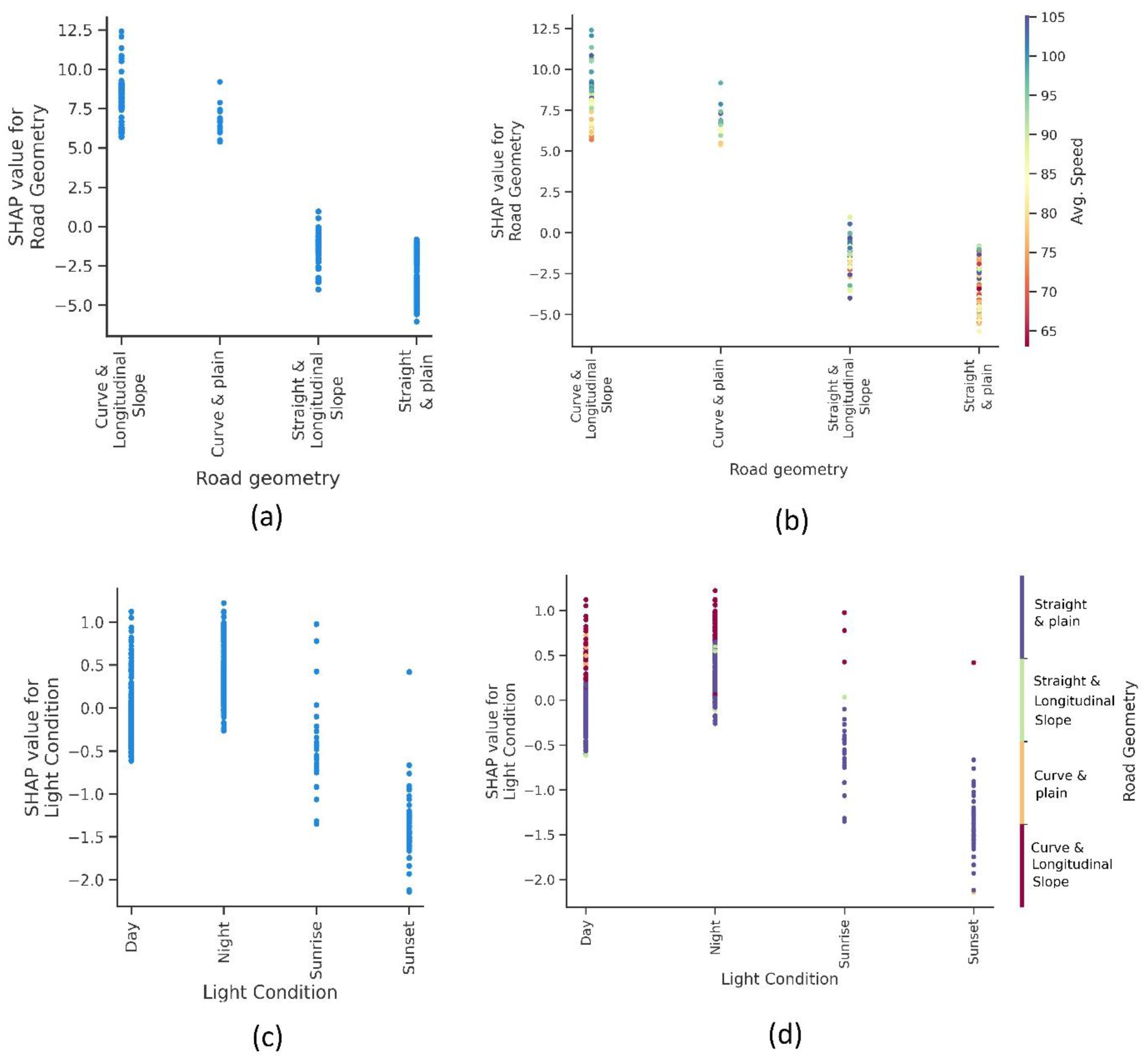
4.3.3. Environmental Factors

This study identified the geometry of the crash location as the most influential variable on PU crash severity. According to the SHAP dependence plots shown in Figure 11a, PU crashes in horizontal curves are associated with positive SHAP values and a higher risk of F&IN PU crashes. Horizontal curves are widely acknowledged as high-risk areas associated with severe crashes [85]. Furthermore, the presence of a longitudinal slope in conjunction with a horizontal curve is associated with elevated SHAP values and a higher risk of severe PU crashes. This is consistent with studies [86,87,88], indicating a correlation between severe crashes and horizontal curves along steep slopes. It appears that due to limited visibility in the combined conditions of horizontal curves and longitudinal slopes, and the difficulty of vehicle control in these geometric conditions, the risk of severe PU crashes increases. Additionally, Figure 11b presents the interaction effect of road geometry and average speed, indicating that the occurrence of crashes in horizontal curves with high average speeds increases the likelihood of PU crashes with F&IN severity.
Based on Figure 11c, the probability of severe PU crashes occurring at night is associated with positive SHAP values and a higher risk of F&IN PU crashes, which could be due to factors such as reduced visibility, inadequate lighting, fatigue, and driver drowsiness. Other studies have also shown a correlation between crashes occurring at night and risk of severe crash [9,89,90,91]. As shown in Figure 11d, the combination of crashes at night and horizontal curves is associated with a higher risk of F&IN PU crashes. Moreover, the combination of horizontal curves and longitudinal slopes during daytime increases the risk of severe PU crashes, whereas straight road segments pose a lower risk (Figure 11d). Therefore, the interaction of nighttime darkness, horizontal curves, and longitudinal slopes is critical, and even during daylight hours, horizontal curves can pose a significant risk for severe PU crashes.

5. Conclusions

PU crashes involve collisions between more than two vehicles and are regarded as dangerous and costly traffic incidents, given their high rates of fatalities and injuries, substantial infrastructure damage, involvement of multiple vehicles, and intricate legal ramifications. Given the superiority of real-time traffic over aggregated traffic variables at the time of crash occurrence and the impact of driving on environmental and roadway conditions, the analysis and modeling of PU crashes focuses on real-time traffic and environmental parameters. Numerous studies have investigated the impact of congestion on safety. However, the results of many of these studies have been qualitative and inconsistent, which can lead to confusion among transport planners and safety policymakers regarding the risky values of congestion. Moreover, while the safety risks associated with heavy vehicles in traffic combinations and their unsafe interactions with other vehicles are well recognized, the impact of their presence on crash severity has received less attention. Therefore, this study aimed to shed further light on the impact of these variables on PU crash severity, including the use of TV/C as a congestion indicator, HVV/TV, and environmental variables and their interactions. In this study, six ML models were implemented and their performance was compared, with the CatBoost model being selected as the best model. The SHAP method was employed to interpret the results obtained from the CatBoost model, and the modeling results of PU crash severity were analyzed to interpret critical risk factors and their interactions. The plots provide information not only on the direction and magnitude of each variable’s impact but also on their criticality with respect to severe crashes.
Through modeling and interpretation of the results, it was found that road geometry, no. of vehicles involved, a v g . s p e e d , T V / C , H V V / T V , no. of heavy vehicles involved, light conditions, road surface conditions, land use, and no. of lanes have an impact on the PU crash severity in order of importance. In general, high average speed, less congestion, and a higher proportion of heavy vehicles in traffic are associated with risk of severe PU crashes. Enforcing stricter speed limit regulations and imposing severe penalties for speeding, while also promoting a culture of safe driving and obeying speed limits, can lead to substantial safety improvements [92]. A relatively new technological approach that is very effective in improving speed compliance and reducing crashes is point-to-point (P2P) speed enforcement, also referred to as average speed enforcement or section speed enforcement, which involves the calculation of the average speed over a section [93,94,95,96]. T V / C < 0.6 is associated with severe PU crashes, and its critical values are about 0.1 (higher vehicle speeds) and 0.45 (higher exposure). For H V V / T V 0.1 , there is a risk of F&IN PU crashes, and the interaction between T V / C 0.1 , H V V / T V 0.25 , and nighttime darkness conditions lead to a high likelihood of severe PU crashes. For all critical congestions ( T V / C 0.1 & 0.45 ), average speeds above 90 km/h are associated with severe PU crashes. Additionally, in conditions with a high percentage of heavy vehicles, an increase in average speed is accompanied by higher SHAP values and a higher risk of severe PU crashes.
The history of T V / C values for various sections of freeways is accessible, which enables the identification of hours and days when TV/C values approach critical levels. By managing traffic during these critical periods and implementing appropriate regulations, traffic authorities can help prevent hazardous traffic conditions. For example, reducing speed in non-congested conditions ( T V / C 0.1 ) or increasing capacity on routes with prolonged periods of critical traffic ( T V / C 0.45 ) can help reduce the likelihood of severe PU crashes. Innovative traffic control systems can also identify critical congestions using the real-time information of detectors [97] and encourage drivers to drive more cautiously through variable message signs. In this study, the SHAP results provide the impact of H V V / T V , which can be used to identify critical traffic conditions for H V V / T V on routes in the real world with online traffic volume data. Furthermore, short-term prediction of truck traffic based on logistics activities [98] and bus traffic by employing a passenger-oriented traffic control strategy [99] is possible. Such predictions can help anticipate critical conditions related to the prevalence of heavy vehicles in traffic and aid in their management. Allocating alternative routes for large trucks and buses or managing the timing and stops of these vehicles to avoid critical traffic conditions can decrease the probability of severe PU crashes.
PU crashes in horizontal curves are associated with severe crashes, and when horizontal curves are combined with longitudinal slopes, the likelihood of severe PU crashes increases. Installing chevrons and edge line rumble strips reduces the occurrence of primary crashes that can lead to subsequent PU crashes [100]. Additionally, the interaction between horizontal curves and high average speeds leads to a likelihood of severe PU crashes. Improving friction [101] and implementing advisory speed limits at curve locations, particularly in sections with high longitudinal grades, can improve safety. Severe PU crashes are more likely to occur at night, and this is often due to reduced visibility during nighttime conditions. The critical condition of PU crash severity involves the interaction between horizontal curves and nighttime darkness. Improving the lighting conditions of the roadway and enhancing the quality and visibility of road markings and signs are effective measures for increasing safety [90].
Examining crash characteristic variables can shed light on post-crash conditions, but understanding how they impact crash severity can inform the development of appropriate safety policies. According to the study results, an increase in the number of heavy vehicles involved increases the probability of severe PU crashes. In PU crashes, it is possible for vehicles to experience multiple impacts and strikes, and secondary impacts may result in severe collisions, especially from heavy vehicles. As a result, it is vital to ensure that vehicles are protected against secondary impacts and that occupants are safeguarded following multiple impacts and vehicle deformations. It is recommended that modern material technologies are utilized in vehicle chassis structures to prevent accumulated plastic deformation resulting from multiple impacts, which can cause harm to occupants in PU crashes [102].

6. Limitations and Future Direction

While this research utilizes crash and traffic data from Iran as a specific case study, the results are shaped by the distinct characteristics of Iran’s freeway infrastructure, environmental conditions, traffic regulations, and driving behaviors. It is important to exercise caution when extrapolating these findings to diverse settings. Nevertheless, the methodology employed in this study can be modified for tackling various challenges. Furthermore, the study relied on traffic variables obtained from loop detectors on Iran’s suburban freeways, recognizing the potential for inaccuracies due to the distances between loop detectors and crash locations. Moreover, while we attempted to address the capacity of each segment, which might be affected by weather, according to the specific weather conditions, it is assumed that the capacity does not change significantly due to other temporal elements, which may result in limited inaccuracies.
Finally, we acknowledge the importance of exploring more comprehensive databases, particularly utilizing high-resolution real-time traffic data in forthcoming studies. This approach could enable the exploration of critical conditions through crash modeling and the derivation of other real-time traffic measures using fundamental diagrams. Furthermore, it would be valuable to examine the effects of time-related variables, including fluctuations in climate, alterations in road infrastructure, and advancements in vehicle safety technology throughout the research duration. Additionally, integrating qualitative inquiries, such as surveys or interviews with drivers to identify potential hazards leading to severe crashes, could provide deep insights into human and behavioral factors.

Author Contributions

Conceptualization: S.A.S. and K.A.; Methodology: S.A.S.; Software: S.A.S.; Validation: K.A. and A.M.; Formal Analysis: S.A.S.; Investigation: K.A.; Data Curation: S.A.S.; Writing—Original Draft Preparation: S.A.S.; Writing—Review and Editing: K.A. and A.M.; Visualization: K.A.; Supervision, K.A. and A.M. All authors have read and agreed to the published version of the manuscript.

Funding

This research received no external funding.

Institutional Review Board Statement

The study was conducted according to the guidelines of the Declaration of Helsinki, and approved by the Ethics Committee of School of Civil Engineering, University of Tehran (number 82-C-489, dated 12 July 2023).

Informed Consent Statement

Not applicable.

Data Availability Statement

The data presented in this study are available on request from the corresponding author. The data are not publicly available due to the policies of the Iran Road Safety Organization.

Conflicts of Interest

The authors declare no conflicts of interest.

References

  1. Lord, D.; Washington, S. Safe Mobility: Challenges, Methodology and Solutions; Emerald Publishing Bingley: West Yorkshire, UK, 2018. [Google Scholar]
  2. WHO—World Health Organization. Global Status Report on Road Safety 2023; World Health Organization, WHO Press: Geneva, Switzerland, 2023. [Google Scholar]
  3. Bakhtiyari, M.; Delpisheh, A.; Monfared, A.B.; Kazemi-Galougahi, M.H.; Mehmandar, M.R.; Riahi, M.; Salehi, M.; Mansournia, M.A. The road traffic crashes as a neglected public health concern; an observational study from Iranian population. Traffic Inj. Prev. 2015, 16, 36–41. [Google Scholar] [CrossRef]
  4. Hosseinzadeh, A.; Moeinaddini, A.; Ghasemzadeh, A. Investigating factors affecting severity of large truck-involved crashes: Comparison of the SVM and random parameter logit model. J. Saf. Res. 2021, 77, 151–160. [Google Scholar] [CrossRef]
  5. Meng, F.; Xu, P.; Song, C.; Gao, K.; Zhou, Z.; Yang, L. Influential factors associated with consecutive crash severity: A two-level logistic modeling approach. Int. J. Environ. Res. Public Health 2020, 17, 5623. [Google Scholar] [CrossRef]
  6. Feng, M.; Wang, X.; Li, Y. Analyzing single-vehicle and multi-vehicle freeway crashes with unobserved heterogeneity. J. Transp. Saf. Secur. 2023, 15, 59–81. [Google Scholar] [CrossRef]
  7. Geedipally, S.R.; Lord, D. Investigating the effect of modeling single-vehicle and multi-vehicle crashes separately on confidence intervals of Poisson–gamma models. Accid. Anal. Prev. 2010, 42, 1273–1282. [Google Scholar] [CrossRef] [PubMed]
  8. Ma, J.; Ren, G.; Li, H.; Wang, S.; Yu, J. Characterizing the differences of injury severity between single-vehicle and multi-vehicle crashes in China. J. Transp. Saf. Secur. 2023, 15, 314–334. [Google Scholar] [CrossRef]
  9. Wu, Q.; Chen, F.; Zhang, G.; Liu, X.C.; Wang, H.; Bogus, S.M. Mixed logit model-based driver injury severity investigations in single- and multi-vehicle crashes on rural two-lane highways. Accid. Anal. Prev. 2014, 72, 105–115. [Google Scholar] [CrossRef]
  10. Zichu, Z.; Fanyu, M.; Cancan, S.; Richard, T.; Zhongyin, G.; Lili, Y.; Weili, W. Factors associated with consecutive and non-consecutive crashes on freeways: A two-level logistic modeling approach. Accid. Anal. Prev. 2021, 154, 106054. [Google Scholar] [CrossRef] [PubMed]
  11. Nagatani, T.; Yonekura, S. Multiple-vehicle collision induced by lane changing in traffic flow. Phys. A Stat. Mech. Appl. 2014, 404, 171–179. [Google Scholar] [CrossRef]
  12. Nagatani, T. Chain-reaction crash in traffic flow controlled by taillights. Phys. A Stat. Mech. Appl. 2015, 419, 1–6. [Google Scholar] [CrossRef]
  13. Xu, C.; Liu, P.; Yang, B.; Wang, W. Real-time estimation of secondary crash likelihood on freeways using high-resolution loop detector data. Transp. Res. Part C Emerg. Technol. 2016, 71, 406–418. [Google Scholar] [CrossRef]
  14. Li, J.; Guo, J.; Wijnands, J.S.; Yu, R.; Xu, C.; Stevenson, M. Assessing injury severity of secondary incidents using support vector machines. J. Transp. Saf. Secur. 2022, 14, 197–216. [Google Scholar] [CrossRef]
  15. Huang, H.; Ding, X.; Yuan, C.; Liu, X.; Tang, J. Jointly analyzing freeway primary and secondary crash severity using a copula-based approach. Accid. Anal. Prev. 2023, 180, 106911. [Google Scholar] [CrossRef] [PubMed]
  16. Mishra, S.; Golias, M.; Sarker, A.; Naimi, A. Effect of Primary and Secondary Crashes: Identification, Visualization, and Prediction; National Center for Freight & Infrastructure Research & Education: Madison, WI, USA, 2016. [Google Scholar]
  17. Zhang, H.; Khattak, A. What is the role of multiple secondary incidents in traffic operations? J. Transp. Eng. 2010, 136, 986–997. [Google Scholar] [CrossRef]
  18. Høye, A.K.; Hesjevoll, I.S. Traffic volume and crashes and how crash and road characteristics affect their relationship—A meta-analysis. Accid. Anal. Prev. 2020, 145, 105668. [Google Scholar] [CrossRef]
  19. Kitali, A.E.; Alluri, P.; Sando, T.; Haule, H.; Kidando, E.; Lentz, R. Likelihood estimation of secondary crashes using Bayesian complementary log-log model. Accid. Anal. Prev. 2018, 119, 58–67. [Google Scholar] [CrossRef]
  20. Park, H.; Haghani, A.; Samuel, S.; Knodler, M.A. Real-time prediction and avoidance of secondary crashes under unexpected traffic congestion. Accid. Anal. Prev. 2018, 112, 39–49. [Google Scholar] [CrossRef]
  21. Li, P.; Abdel-Aty, M. A hybrid machine learning model for predicting Real-Time secondary crash likelihood. Accid. Anal. Prev. 2022, 165, 106504. [Google Scholar] [CrossRef]
  22. Yu, R.; Abdel-Aty, M. Analyzing crash injury severity for a mountainous freeway incorporating real-time traffic and weather data. Saf. Sci. 2014, 63, 50–56. [Google Scholar] [CrossRef]
  23. Yu, R.; Abdel-Aty, M. Using hierarchical Bayesian binary probit models to analyze crash injury severity on high speed facilities with real-time traffic data. Accid. Anal. Prev. 2014, 62, 161–167. [Google Scholar] [CrossRef] [PubMed]
  24. Lord, D.; Manar, A.; Vizioli, A. Modeling crash-flow-density and crash-flow-V/C ratio relationships for rural and urban freeway segments. Accid. Anal. Prev. 2005, 37, 185–199. [Google Scholar] [CrossRef]
  25. Quddus, M.A.; Wang, C.; Ison, S.G. Road traffic congestion and crash severity: Econometric analysis using ordered response models. J. Transp. Eng. 2010, 136, 424–435. [Google Scholar] [CrossRef]
  26. Wang, C.; Quddus, M.; Ison, S. A spatio-temporal analysis of the impact of congestion on traffic safety on major roads in the UK. Transp. A Transp. Sci. 2013, 9, 124–148. [Google Scholar] [CrossRef]
  27. Apley, D.W.; Zhu, J. Visualizing the effects of predictor variables in black box supervised learning models. J. R. Stat. Soc. Ser. B (Stat. Methodol.) 2020, 82, 1059–1086. [Google Scholar] [CrossRef]
  28. Silva, P.B.; Andrade, M.; Ferreira, S. Machine learning applied to road safety modeling: A systematic literature review. J. Traffic Transp. Eng. (Engl. Ed.) 2020, 7, 775–790. [Google Scholar] [CrossRef]
  29. Prati, G.; Pietrantoni, L.; Fraboni, F. Using data mining techniques to predict the severity of bicycle crashes. Accid. Anal. Prev. 2017, 101, 44–54. [Google Scholar] [CrossRef] [PubMed]
  30. López, G.; Abellán, J.; Montella, A.; de Oña, J. Patterns of Single-Vehicle Crashes on Two-Lane Rural Highways in Granada Province, Spain: In-Depth Analysis through Decision Rules. Transp. Res. Rec. 2014, 2432, 133–141. [Google Scholar] [CrossRef]
  31. Montella, A.; Aria, M.; D’Ambrosio, A.; Mauriello, F. Data-Mining Techniques for Exploratory Analysis of Pedestrian Crashes. Transp. Res. Rec. 2011, 2237, 107–116. [Google Scholar] [CrossRef]
  32. Montella, A.; de Oña, R.; Mauriello, F.; Rella Riccardi, M.; Silvestro, G. A data mining approach to investigate patterns of pow-ered two-wheeler crashes in Spain. Accid. Anal. Prev. 2020, 134, 105251. [Google Scholar] [CrossRef] [PubMed]
  33. Montella, A.; Mauriello, F.; Pernetti, M.; Rella Riccardi, M. Rule discovery to identify patterns contributing to overrepresentation and severity of run-off-the-road crashes. Accid. Anal. Prev. 2021, 155, 106119. [Google Scholar] [CrossRef] [PubMed]
  34. Moral-Garcia, S.; Castellano, J.G.; Mantas, J.G.; Montella, A.; Abellan, J. Decision tree ensemble method for analyzing traffic accidents of novice drivers in urban areas. Entropy 2019, 21, 360. [Google Scholar] [CrossRef]
  35. Rella Riccardi, M.; Galante, F.; Scarano, A.; Montella, A. Econometric and machine learning methods to identify pedestrian crash patterns. Sustainability 2022, 14, 15471. [Google Scholar] [CrossRef]
  36. Rella Riccardi, M.; Mauriello, F.; Scarano, A.; Montella, A. Analysis of contributory factors of fatal pedestrian crashes by mixed logit model and association rules. Int. J. Inj. Control Saf. Promot. 2023, 30, 195–209. [Google Scholar] [CrossRef]
  37. Iranitalab, A.; Khattak, A. Comparison of four statistical and machine learning methods for crash severity prediction. Accid. Anal. Prev. 2017, 108, 27–36. [Google Scholar] [CrossRef]
  38. Santos, K.; Dias, J.P.; Amado, C. A literature review of machine learning algorithms for crash injury severity prediction. J. Saf. Res. 2021, 80, 254–269. [Google Scholar] [CrossRef]
  39. Rella Riccardi, M.; Mauriello, F.; Sarkar, S.; Galante, F.; Scarano, A.; Montella, A. Parametric and Non-Parametric Analyses for Pedestrian Crash Severity Prediction in Great Britain. Sustainability 2022, 14, 3188. [Google Scholar] [CrossRef]
  40. Scarano, A.; Rella Riccardi, M.; Mauriello, F.; D’Agostino, C.; Pasquino, N.; Montella, A. Injury severity prediction of cyclist crashes using random forests and random parameters logit models. Accid. Anal. Prev. 2023, 192, 107275. [Google Scholar] [CrossRef] [PubMed]
  41. Zhu, S. Analysis of the severity of vehicle-bicycle crashes with data mining techniques. J. Saf. Res. 2021, 76, 218–227. [Google Scholar] [CrossRef]
  42. Scarano, A.; Aria, M.; Mauriello, F.; Rella Riccardi, M.; Montella, A. Systematic literature review of 10 years of cyclist safety research. Accid. Anal. Prev. 2023, 184, 106996. [Google Scholar] [CrossRef]
  43. Dong, S.; Khattak, A.; Ullah, I.; Zhou, J.; Hussain, A. Predicting and analyzing road traffic injury severity using boosting-based ensemble learning models with SHAPley Additive exPlanations. Int. J. Environ. Res. Public Health 2022, 19, 2925. [Google Scholar] [CrossRef] [PubMed]
  44. Hasan, A.S.; Jalayer, M.; Das, S.; Kabir, M.A.B. Application of Machine Learning Models and SHAP to Examine Crashes Involving Young Drivers in New Jersey. Int. J. Transp. Sci. Technol. 2023; in press. [Google Scholar]
  45. Lin, C.; Wu, D.; Liu, H.; Xia, X.; Bhattarai, N. Factor identification and prediction for teen driver crash severity using machine learning: A case study. Appl. Sci. 2020, 10, 1675. [Google Scholar] [CrossRef]
  46. Ma, Z.; Mei, G.; Cuomo, S. An analytic framework using deep learning for prediction of traffic accident injury severity based on contributing factors. Accid. Anal. Prev. 2021, 160, 106322. [Google Scholar] [CrossRef]
  47. Wen, X.; Xie, Y.; Wu, L.; Jiang, L. Quantifying and comparing the effects of key risk factors on various types of roadway segment crashes with LightGBM and SHAP. Accid. Anal. Prev. 2021, 159, 106261. [Google Scholar] [CrossRef]
  48. Xu, G.; Duong, T.D.; Li, Q.; Liu, S.; Wang, X. Causality learning: A new perspective for interpretable machine learning. arXiv 2020, arXiv:2006.16789. [Google Scholar]
  49. Mussone, L.; Bassani, M.; Masci, P. Analysis of factors affecting the severity of crashes in urban road intersections. Accid. Anal. Prev. 2017, 103, 112–122. [Google Scholar] [CrossRef] [PubMed]
  50. Tang, J.; Liang, J.; Han, C.; Li, Z.; Huang, H. Crash injury severity analysis using a two-layer Stacking framework. Accid. Anal. Prev. 2019, 122, 226–238. [Google Scholar] [CrossRef]
  51. Wang, X.; Kim, S.H. Prediction and factor identification for crash severity: Comparison of discrete choice and tree-based models. Transp. Res. Rec. 2019, 2673, 640–653. [Google Scholar] [CrossRef]
  52. Friedman, J.H. Greedy function approximation: A gradient boosting machine. Ann. Stat. 2001, 29, 1189–1232. [Google Scholar] [CrossRef]
  53. Toran Pour, A.; Moridpour, S.; Tay, R.; Rajabifard, A. Modelling pedestrian crash severity at mid-blocks. Transp. A Transp. Sci. 2017, 13, 273–297. [Google Scholar] [CrossRef]
  54. Masís, S. Interpretable Machine Learning with Python: Learn to Build Interpretable High-Performance Models with Hands-On Real-World Examples; Packt Publishing Ltd.: Birmingham, UK, 2021. [Google Scholar]
  55. Molnar, C. Interpretable Machine Learning; Lulu. com: Raleigh, NC, USA, 2020. [Google Scholar]
  56. Lundberg, S.M.; Lee, S.-I. A unified approach to interpreting model predictions. In Advances in Neural Information Processing Systems, Proceedings of the NIPS 2017, Long Beach, CA, USA, 4–9 December 2017; NeurIPS: Long Beach, CA, USA, 2017; Volume 30. [Google Scholar]
  57. Parsa, A.B.; Movahedi, A.; Taghipour, H.; Derrible, S.; Mohammadian, A.K. Toward safer highways, application of XGBoost and SHAP for real-time accident detection and feature analysis. Accid. Anal. Prev. 2020, 136, 105405. [Google Scholar] [CrossRef] [PubMed]
  58. Yang, C.; Chen, M.; Yuan, Q. The application of XGBoost and SHAP to examining the factors in freight truck-related crashes: An exploratory analysis. Accid. Anal. Prev. 2021, 158, 106153. [Google Scholar] [CrossRef]
  59. IRMTO—Iran Road Maintenance and Transportation Organization; Minestry of Roads and Urban Development. 2023. Available online: https://rmto.ir/en/ (accessed on 15 July 2023).
  60. Theofilatos, A. Incorporating real-time traffic and weather data to explore road accident likelihood and severity in urban arterials. J. Saf. Res. 2017, 61, 9–21. [Google Scholar] [CrossRef] [PubMed]
  61. Theofilatos, A.; Ziakopoulos, A. Traffic Flow Volume and Safety. In International Encyclopedia of Transportation; Vickerman, R., Ed.; Elsevier: Oxford, UK, 2021; pp. 692–698. [Google Scholar]
  62. Elvik, R.; Vadeby, A.; Hels, T.; van Schagen, I. Updated estimates of the relationship between speed and road safety at the aggregate and individual levels. Accid. Anal. Prev. 2019, 123, 114–122. [Google Scholar] [CrossRef] [PubMed]
  63. Breiman, L. Random Forests. Mach. Learn. 2001, 45, 5–32. [Google Scholar] [CrossRef]
  64. Chen, T.; Guestrin, C. Xgboost: A scalable tree boosting system. In Proceedings of the 22nd ACM SIGKDD International Conference on Knowledge Discovery and Data Mining, San Francisco, CA, USA, 13–17 August 2016; pp. 785–794. [Google Scholar]
  65. Hancock, J.T.; Khoshgoftaar, T.M. CatBoost for big data: An interdisciplinary review. J. Big Data 2020, 7, 94. [Google Scholar] [CrossRef] [PubMed]
  66. Ke, G.; Meng, Q.; Finley, T.; Wang, T.; Chen, W.; Ma, W.; Ye, Q.; Liu, T.-Y. Lightgbm: A highly efficient gradient boosting decision tree. In Advances in Neural Information Processing Systems, Proceedings of the NIPS 2017, Long Beach, CA, USA, 4–9 December 2017; NeurIPS: Long Beach, CA, USA, 2017; Volume 30. [Google Scholar]
  67. Wang, F.; Jiang, D.; Wen, H.; Song, H. Adaboost-based security level classification of mobile intelligent terminals. J. Supercomput. 2019, 75, 7460–7478. [Google Scholar] [CrossRef]
  68. Dorogush, A.V.; Ershov, V.; Gulin, A. CatBoost: Gradient boosting with categorical features support. arXiv 2018, arXiv:1810.11363. [Google Scholar]
  69. Hussain, S.; Mustafa, M.W.; Jumani, T.A.; Baloch, S.K.; Alotaibi, H.; Khan, I.; Khan, A. A novel feature engineered-CatBoost-based supervised machine learning framework for electricity theft detection. Energy Rep. 2021, 7, 4425–4436. [Google Scholar] [CrossRef]
  70. Morris, C.; Yang, J.J. Effectiveness of resampling methods in coping with imbalanced crash data: Crash type analysis and predictive modeling. Accid. Anal. Prev. 2021, 159, 106240. [Google Scholar] [CrossRef]
  71. Ying, X. An overview of overfitting and its solutions. Proc. J. Phys. Conf. Ser. 2019, 1168, 022022. [Google Scholar] [CrossRef]
  72. Štrumbelj, E.; Kononenko, I. Explaining prediction models and individual predictions with feature contributions. Knowl. Inf. Syst. 2014, 41, 647–665. [Google Scholar] [CrossRef]
  73. Lundberg, S.; Erion, G.; Chen, H.; DeGrave, A.; Prutkin, J.; Nair, B.; Katz, R.; Himmelfarb, J.; Bansal, N.; Lee, S. From local explanations to global understanding with explainable AI for trees. Nat. Mach. Intell. 2020, 2, 56–67. [Google Scholar] [CrossRef]
  74. Ahmed, S.S.; Alnawmasi, N.; Anastasopoulos, P.C.; Mannering, F. The effect of higher speed limits on crash-injury severity rates: A correlated random parameters bivariate tobit approach. Anal. Methods Accid. Res. 2022, 34, 100213. [Google Scholar] [CrossRef]
  75. Alnawmasi, N.; Mannering, F. The impact of higher speed limits on the frequency and severity of freeway crashes: Accounting for temporal shifts and unobserved heterogeneity. Anal. Methods Accid. Res. 2022, 34, 100205. [Google Scholar] [CrossRef]
  76. Hasan, A.S.; Orvin, M.M.; Jalayer, M.; Heitmann, E.; Weiss, J. Analysis of distracted driving crashes in New Jersey using mixed logit model. J. Saf. Res. 2022, 81, 166–174. [Google Scholar] [CrossRef] [PubMed]
  77. Khan, G.; Bill, A.R.; Noyce, D.A. Exploring the feasibility of classification trees versus ordinal discrete choice models for analyzing crash severity. Transp. Res. Part C Emerg. Technol. 2015, 50, 86–96. [Google Scholar] [CrossRef]
  78. Mohanty, M.; Panda, B.; Dey, P.P. Quantification of surrogate safety measure to predict severity of road crashes at median openings. IATSS Res. 2021, 45, 153–159. [Google Scholar] [CrossRef]
  79. Xu, C.; Tarko, A.P.; Wang, W.; Liu, P. Predicting crash likelihood and severity on freeways with real-time loop detector data. Accid. Anal. Prev. 2013, 57, 30–39. [Google Scholar] [CrossRef]
  80. Harwood, D.W.; Bauer, K.M.; Potts, I.B. Development of Relationships between Safety and Congestion for Urban Freeways. Transp. Res. Rec. 2013, 2398, 28–36. [Google Scholar] [CrossRef]
  81. Jo, Y.; Oh, C.; Kim, S. Estimation of heavy vehicle-involved rear-end crash potential using WIM data. Accid. Anal. Prev. 2019, 128, 103–113. [Google Scholar] [CrossRef]
  82. Hyun, K.; Jeong, K.; Tok, A.; Ritchie, S.G. Assessing crash risk considering vehicle interactions with trucks using point detector data. Accid. Anal. Prev. 2019, 130, 75–83. [Google Scholar] [CrossRef] [PubMed]
  83. Wu, J.; Rasouli, S.; Zhao, J.; Qian, Y.; Cheng, L. Large truck fatal crash severity segmentation and analysis incorporating all parties involved: A Bayesian network approach. Travel Behav. Soc. 2023, 30, 135–147. [Google Scholar] [CrossRef]
  84. Zhu, X.; Srinivasan, S. A comprehensive analysis of factors influencing the injury severity of large-truck crashes. Accid. Anal. Prev. 2011, 43, 49–57. [Google Scholar] [CrossRef]
  85. Rakotonirainy, A.; Chen, S.; Scott-Parker, B.; Loke, S.W.; Krishnaswamy, S. A novel approach to assessing road-curve crash severity. J. Transp. Saf. Secur. 2015, 7, 358–375. [Google Scholar] [CrossRef]
  86. Wang, Y.; Zhang, W. Analysis of Roadway and Environmental Factors Affecting Traffic Crash Severities. Transp. Res. Procedia 2017, 25, 2119–2125. [Google Scholar] [CrossRef]
  87. Rusli, R.; Haque, M.M.; Saifuzzaman, M.; King, M. Crash severity along rural mountainous highways in Malaysia: An application of a combined decision tree and logistic regression model. Traffic Inj. Prev. 2018, 19, 741–748. [Google Scholar] [CrossRef] [PubMed]
  88. Wen, H.; Ma, Z.; Chen, Z.; Luo, C. Analyzing the impact of curve and slope on multi-vehicle truck crash severity on mountainous freeways. Accid. Anal. Prev. 2023, 181, 106951. [Google Scholar] [CrossRef]
  89. Abegaz, T.; Berhane, Y.; Worku, A.; Assrat, A.; Assefa, A. Effects of excessive speeding and falling asleep while driving on crash injury severity in Ethiopia: A generalized ordered logit model analysis. Accid. Anal. Prev. 2014, 71, 15–21. [Google Scholar] [CrossRef]
  90. Ackaah, W.; Apuseyine, B.A.; Afukaar, F.K. Road traffic crashes at night-time: Characteristics and risk factors. Int. J. Inj. Control Saf. Promot. 2020, 27, 392–399. [Google Scholar] [CrossRef]
  91. Yannis, G.; Athanasios, T.; George, P. Investigation of road accident severity per vehicle type. Transp. Res. Procedia 2017, 25, 2076–2083. [Google Scholar] [CrossRef]
  92. Yasmin, S.; Eluru, N.; Haque, M.M. Addressing endogeneity in modeling speed enforcement, crash risk and crash severity simultaneously. Anal. Methods Accid. Res. 2022, 36, 100242. [Google Scholar] [CrossRef]
  93. Montella, A.; Persaud, B.; D’Apuzzo, M.; Imbriani, L.L. Safety Evaluation of an Automated Section Speed Enforcement System. Transp. Res. Rec. 2012, 2281, 16–25. [Google Scholar] [CrossRef]
  94. Montella, A.; Imbriani, L.L.; Marzano, V.; Mauriello, F. Effects on speed and safety of point-to-point speed enforcement systems: Evaluation on the urban motorway A56 Tangenziale di Napoli. Accid. Anal. Prev. 2015, 75, 164–178. [Google Scholar] [CrossRef] [PubMed]
  95. Montella, A.; Punzo, V.; Chiaradonna, S.; Mauriello, F.; Montanino, M. Point-to-point speed enforcement systems: Speed limits design criteria and analysis of drivers’ compliance. Transp. Res. Part C Emerg. Technol. 2015, 53, 1–18. [Google Scholar] [CrossRef]
  96. Soole, D.W.; Watson, B.C.; Fleiter, J.J. Effects of average speed enforcement on speed compliance and crashes: A review of the literature. Accid. Anal. Prev. 2013, 54, 46–56. [Google Scholar] [CrossRef]
  97. Ahmed, F.; Hawas, Y.E. An integrated real-time traffic signal system for transit signal priority, incident detection and congestion management. Transp. Res. Part C Emerg. Technol. 2015, 60, 52–76. [Google Scholar] [CrossRef]
  98. Nadi, A.; Sharma, S.; Snelder, M.; Bakri, T.; van Lint, H.; Tavasszy, L. Short-term prediction of outbound truck traffic from the exchange of information in logistics hubs: A case study for the port of Rotterdam. Transp. Res. Part C Emerg. Technol. 2021, 127, 103111. [Google Scholar] [CrossRef]
  99. Chen, S.; Fu, H.; Wu, N.; Wang, Y.; Qiao, Y. Passenger-oriented traffic management integrating perimeter control and regional bus service frequency setting using 3D-pMFD. Transp. Res. Part C Emerg. Technol. 2022, 135, 103529. [Google Scholar] [CrossRef]
  100. Islam, M.; Hosseini, P.; Jalayer, M. An analysis of single-vehicle truck crashes on rural curved segments accounting for unobserved heterogeneity. J. Saf. Res. 2022, 80, 148–159. [Google Scholar] [CrossRef]
  101. Cafiso, S.; Montella, A.; D’Agostino, C.; Mauriello, F.; Galante, F. Crash modification functions for pavement surface condition and geometric design indicators. Accid. Anal. Prev. 2021, 149, 105887. [Google Scholar] [CrossRef]
  102. Liu, Q.; Shen, H.; Wu, Y.; Xia, Z.; Fang, J.; Li, Q. Crash responses under multiple impacts and residual properties of CFRP and aluminum tubes. Compos. Struct. 2018, 194, 87–103. [Google Scholar] [CrossRef]
Figure 1. Study routes: 1: Tehran–Qom (150 km), 2: Qom–Isfahan (360 km), 3: Tehran–Qazvin (120 km), 4: Tehran–Saveh (95 Km), 5: Qazvin–Tabriz (490 km), 6: Qazvin–Rasht (160 km), 7: Saveh–Hamadan (175 km), 8: Saveh–Salafchegan (80 Km), 9: Qom–Garmsar (150 km), 10: Khoramabad–Andimeshk (145 km), 11: Ahvaz–BandarImam (90 km).
Safety 10 00022 g001
Figure 2. Kernel density plot of real-time traffic variables: (a) TV/C; (b) HVV/TV; (c) avg.speed.
Safety 10 00022 g002
Figure 3. Matrix Scatter plot of real-time traffic variables.
Safety 10 00022 g003
Figure 4. Distribution and F&IN rate of PU crashes by number of vehicles involved: (a) all vehicles; (b) heavy vehicles.
Safety 10 00022 g004
Figure 5. Oversampled distribution and F&IN rate of PU crashes by number of vehicles involved.
Safety 10 00022 g005
Figure 6. (a) Variable importance; (b) SHAP summary plot.
Safety 10 00022 g006
Figure 7. Main effects of real-time traffic variables: (a) Avg.speed; (b) T V / C ; (c) H V V / T V .
Safety 10 00022 g007
Figure 8. SHAP main and interaction effect plots: (a) main effect of T V / C ; (b) interaction with avg.speed; (c) interaction with H V V / T V ; (d) interaction with light condition.
Safety 10 00022 g008
Figure 9. SHAP main and interaction effect plots of H V V / T V : (a) main effect; (b) interaction with avg.speed.
Safety 10 00022 g009
Figure 10. SHAP main effect plots of crash characteristics: (a) main effect of no. of vehicles involved; (b) main effect of no. of heavy vehicles involved.
Safety 10 00022 g010
Figure 11. SHAP main and interaction effect plots of environmental factors: (a) main effects of road geometry; (b) interaction effects of road geometry with avg.speed; (c) main effects of light conditions; (d) interaction effects of light conditions with road geometry.
Safety 10 00022 g011
Table 1. Descriptive statistics of variables.
VariableDescriptionPDOF & INTotalMeanStd. DevMinMax
Real-Time Traffic Variables
TV/C 0.4690.2970.0050.98
Avg.speed 84.70 12.77 60 120
HVV/TV 0.1430.1020.0140.634
Crash Characteristics
No. of vehicles involved 3.240.574312
No. of heavy vehicles involved 0.570.79103
No. of injuries 0.150.53706
No. of fatalities 0.020.20305
Environmental Characteristics
NO. Lanes224 (23.07%)80 (76.92%)104 (4.80%)
3393 (19.06%)1668 (80.93%)2061 (95.1%)
Light ConditionDay191 (14.81%)1098 (85.18%)1289 (59.5%)
Night213 (27.41%)564 (72.58%)777 (35.8%)
Sunrise7 (23.33%)23 (76.66%)30 (1.38%)
Sunset6 (8.695%)63 (91.30%)69 (3.18%)
Road Surface ConditionDry321 (18.03%)1459 (81.96%)1780 (82.2%)
Ice and snow15 (24.19%)47 (75.80%)62 (2.86%)
Wet81 (25.07%)242 (74.92%)323 (14.9%)
Land UseAgriculture96 (39.18%)149 (60.81%)245 (11.3%)
Industrial9 (21.42%)33 (78.57%)42 (1.93%)
Other305 (16.38%)1556 (83.61%)1861 (85.9%)
Residential7 (41.17%)10 (58.82%)17 (0.78%)
Weather ConditionCloudy and foggy and dusty15 (33.33%)30 (66.66%)45 (2.07%)
Rainy73 (24.74%)222 (75.25%)295 (13.6%)
Smooth309 (17.60%)1446 (82.39%)1755 (81.0%)
Snow19 (27.53%)50 (72.46%)69 (3.18%)
Storm1 (100%)0 (0%)1 (0.04%)
Road GeometryCurve and longitudinal slope101 (95.28%)5 (4.716%)106 (4.89%)
Curve and plain21 (95.45%)1 (4.545%)22 (1.01%)
Straight and longitudinal slope19 (22.35%)66 (77.64%)85 (3.92%)
Straight and plain276 (14.13%)1676 (85.86%)1952 (90.1%)
Table 2. Confusion matrix.
Predicted
ObservedPositiveNegative
PositiveTPFN
NegativeFPTN
TotalPN
Note: FN = false negative; FP = false positive; TN = true negative; TP = true positive.
Table 3. Model accuracy results.
Model
(Oversampled Data)
AccuracyRecallPrecisionF1 ScoreROC-AUC
CART73.1%0.0%0.0%0.0%50.0%
RF95.0%87.1%93.8%90.3%92.5%
CatBoost95.6%87.6%95.6%91.4%93.1%
XGBoost95.3%85.7%96.3%90.7%92.2%
LightGBM95.3%86.7%95.2%90.8%92.6%
AdaBoost95.3%86.0%96.3%90.9%92.4%
Disclaimer/Publisher’s Note: The statements, opinions and data contained in all publications are solely those of the individual author(s) and contributor(s) and not of MDPI and/or the editor(s). MDPI and/or the editor(s) disclaim responsibility for any injury to people or property resulting from any ideas, methods, instructions or products referred to in the content.

