Biomagnetic Flow with CoFe₂O₄ Magnetic Particles through an Unsteady Stretching/Shrinking Cylinder

Abstract

The study of biomagnetic fluid flow and heat transfer containing magnetic particles through an unsteady stretching/shrinking cylinder was numerically investigated in this manuscript. Biomagnetic fluid namely blood taken as base fluid and CoFe₂O₄ as magnetic particles. Where blood acts as an electrically conducting fluid along with magnetization/polarization. The main concentration is to study a time-dependent biomagnetic fluid flow with magnetic particles that passed through a two dimensional stretching/shrinking cylinder under the influence of thermal radiation, heat source and partial slip condition which has not been studied yet as far as best knowledge of authors. This model is consistent with the principles of magnetohydrodynamic and ferrohydrodynamic. The flow equations, such as momentum, energy which is described physically by a system of coupled, nonlinear partial differential equation with appropriate boundary conditions and converted into a nonlinear system of ordinary differential equations by using suitable similarity transformations. The resultant ODEs numerically solved by applying by applying an efficient numerical technique based on a common finite differencing method along with central differencing, tridiagonal matrix manipulation and an iterative procedure. The values assigned to the parameters are compatible with human body conditions. The numerous results concerning velocity, temperature and pressure field, as well as the skin friction and the rate of heat transfer, are presented for the parameters exhibiting physical significance, such as ferromagnetic interaction parameter, magnetic field parameter, volume fraction, unsteady parameter, curvature parameter, etc. The main numerical findings are that the fluid velocity is decreased as the ferromagnetic number is enhanced gradually in both stretching or shrinking cases whereas, the opposite behavior is found for the skin friction coefficient. The rate of heat transfer with ferromagnetic interaction parameter was also monitored and found that opposite behavior occurs for stretching and shrinking cases. Comparisons were made to check the accuracy of the present numerical results with published literature and found to be in excellent agreement. Hopefully, this proposed model will control the blood flow rate, as well as the rate of heat transfer, such as magnetic hyperthermia.

1. Introduction

The study of biomagnetic fluid dynamic (BFD) has attained serious attention from researchers over the last few decades because of its wide range of applications in the biomedical and bioengineering sector including magnetic resonance imaging (MRI), in cancer therapy (hyperthermia), magnetic drug and gene delivery, magnetic separation, reducing blood during surgeries, tissue engineering as early mentioned by [1,2,3,4,5] as theoretically and experimentally. However, to the author’s best knowledge, the study of a biomagnetic fluid model (blood flow model) containing magnetic particles through an unsteady stretching/shrinking cylindrical has not been studied yet so far. Thus, the main concern is to fill up this gap from the present analysis. The reason behind that is that magnetic particles play a vital role in modern medicine and pharmacology areas due to unique magnetic features which are not present in other materials. For example, in cancer treatment magnetic particles are transferred into cancer cells and enhance the heat (using the hyperthermia therapy method) in presence of an applied magnetic field. As a result, the tumor cells are shrunk without any prejudice of normal tissue and the overall therapy is covered at a very low cost. The most common example of biomagnetic fluid is blood. Blood is deliberated as magnetic fluid due to the presence of red blood cells that contain the hemoglobin molecule which is also a form of iron oxide that is present at a uniquely high concentration in the mature red blood cells [5,6].

Owing to its potential applications in biomedical and bioengineering, many researchers proposed a mathematical model of the biomagnetic fluid model. Basically, the biomagnetic fluid model which is also known as the blood flow model consists of consideration of the principles of magnetohydrodynamic (MHD) and ferrohydrodynamic (FHD). Based on the principle of ferrohydrodynamic (FHD), Haik et al. [5] were the first to construct a mathematical model of biomagnetic fluid. Later on, Tzirtzilakis [6] developed a model of the biomagnetic fluid model under modification of the model of [5] which included both principles of magnetohydrodynamic and ferrohydrodynamic, where blood was considered as biomagnetic fluid and acted as an electrically conducting magnetic fluid. The behavior of electrically non-conducting bloodflow in an aneurysm geometry in the presence of a magnetic dipole was investigated by Tzirtzilakis [7]. Jamalabadi et al. [8] analyzed a biomagnetic blood carreau fluid flow model through a stenosis artery considering the principles of magnetohydrodynamics and ferrohydrodynamics and they also reveal that wall temperature can keep controlled if the blood temperature is below 40 °C. Recently, the effect of variable fluid properties on the BFD model through a three dimensional stretching surface under the influence of magnetic dipole was conducted by Murtaza et al. [9]. Where Murtaza et al. [10] proposed a BFD model which is consistent with the principle of FHD and MHD and in that study they found that the effect of FHD is equally significant to that of MHD. The behavior of an unsteady blood flow model over a three-dimensional stretching/shrinking surface taking into account the FHD and MHD principles was studied by Murtaza et al. [11]. Flow and heat transfer of biomagnetic visco-elastic fluid which is electrically non-conducting through a channel with stretching walls in the presence of magnetic dipole was investigated by Misra et al. [12] and they found that blood velocity in the normal physiological state may be reduced (lowered) when a strong magnetic field of intensity is applied. Misra et al. [13] proposed a mathematical model of radiative MHD blood flow and heat transfer over an unsteady stretching sheet considering the effect of partial slip effects. Moreover, Misra et al. [14] proposed a mathematical model of BFD, where they show that cancerous tissue may be destroyed when exposed to a temperature of 42 °C, while normal tissue is maintained at a suitable temperature. Sushma et al. [15] developed a theoretical analysis study of unsteady MHD blood flow in a permeable vessel under the effect of slip flow conditions and heat source/sink. They found that fluid (blood) velocity near the wall decreased as values of slip parameter increased. Ferdows et al. [16] discussed the BFD flow through a stretched cylinder in the presence of a magnetic dipole. Where, they concluded that blood flow was effectively reduced in the case of BFD formulation rather than MHD and FHD formulation; while in the temperature profile BFD formulation is significantly enhanced rather than that of MHD and FHD. Additionally, blood velocity reduced and temperature distribution increased with the curvature parameter while the values of the FHD parameter were considered larger.

The term nanofluid means that regular fluid, such aswater, oil mixed with one kind of nanoparticles was introduced by Choi et al. [17]. It’s found initially that the thermo-physical correlation for the nanofluid was initiated by Pak et al. [18]. The mathematical model of nanofluid in boundary layer flow and heat transfer was proposed by several researchers. For example, Qasim et al. [19] examined the water-based nanofluid model over a stretching cylinder considering two types of nanoparticles; one was magnetic particles (Fe₃O₄) and the other one was non-magnetic particles (Al₂O₃) in presence of prescribed heat flux. In that study, they showed that the rate of heat transfer gets higher for Al₂O₃ comparable to that with Fe₃O₄ in the case of when the magnetic field is absent. Singh et al. [20] investigated the behavior of Cu-H₂O flow and heat transfer through a stretchable porous cylinder and numerical solutions obtained with aid of the Keller box method. Note that in numerical computation they considered the value of volume fraction of nanoparticles up to 25%. Malik et al. [21] studied the model of sisko fluid flow over a non-linear stretchable cylinder with existing Cattaneo-Christov heat flux. Abbas et al. [22] demonstrated a mathematical model of unsteady flow and heat transfer through a stretching/shrinking cylinder along with partial slip condition and suction. Further, the effect of joule heating and heat source/sink on radiative mixed convection maxwell nanofluid flow through a stretching cylinder was studied by Islam et al. [23]. In this manuscript, the authors solved the system of ODEs with the help of the HAM method. Salahuddin et al. [24] analyzed MHD carreau nanofluid over a stretching cylinder in the presence of reactive species and slip effect and later on this model was numerically solved by using the implicit finite difference method which is also known as the Keller box method. The flow of hydromagnetic nanofluid over a stretching cylinder was conducted by Zeeshan et al. [25]. Alsorynejad et al. [26] applied the fourth-order Runge-Kutta method in order to investigate the effect of MHD Cu/Ag/Al₂O₃/TiO₂-water nanofluid flow over a stretching sheet. Gangadhar et al. [27] examined the Cattaneo-Christov flux model through a stretching cylinder with slip effects where water was assumed as the base fluid and Cu, Ag, Al₂O₃, TiO₂ were taken as nanoparticles and the governing set of ODEs of this problem numerically solved by utilizing the SRM technique.

Nanoparticles offer a very large surface area for heat transfer due to their unique features, such as lower density, excellent physical and chemical stability, etc. Basically, nanofluids are a combination of nanoparticles and base fluid, such as oil, water, etc. Blood can also be considered nanofluid [5,6,10]. Generally, the base fluid contains small volumetric quantities of nanoparticles sized and it’s around 1 to 100 (nm) in diameter when the typical diameter of an atom is between 0.15 and 0.6 nm. Based on their size, nanoparticles may have different shapes, such as cylindrical, spherical, etc. One of the most important effects of using nanoparticles with regular fluid is that the thermal conductivity of nanofluids seems to be remarkably enhanced as compared to regular fluid. Such kind of experimental studies is found in [28,29,30] where they reported that thermal conductivity and dynamical viscosity of nanofluids are functions of the types of nanoparticles along with their shape and size. A theoretical and analytical study of two dimensional couple stress nanofluid flow through a stretched surface along with gyrotratic microorganisms under the influence of thermal radiation was conducted by Khan et al. [31]. They conclude that the temperature of nanoparticles enhanced with the Brownian constant and thermophoresis parameter while reducing for couple stress parameter. Kolsi et al. [32] present a three dimensional MHD nanofluid flow and heat transfer over a stretching and shrinking sheet. While water is considered as a base fluid and Copper and Alumina are nanoparticles. In that study, they found that particle volume fraction plays a significant role in fluid velocity and temperature distributions and shows that in both cases, i.e., upper and lower, increased when values of volume fraction gradually increased. Abbasi et al. [33] studied thermal applications of radiative Casson nanoparticles flow near oblique stagnation point which also considered in cylindrical coordinate systems and the numerical calculations of this problem were solved by using MATLAB (in abbreviation of MATrix LABoratory, MathWorks, Natick, MA, USA) 2018b software with boundary value problem solver (bvp4c) technique.

From the analysis of the above study, the interesting finding is that the study of biological fluid containing magnetic particles through an unsteady stretching/shrinking cylinder under slip effect has not yet been studied to the authors’ knowledge. The main target throughout this study is to fill up this gap by numerical investigation. The present model is known as Biomagnetic Fluid Dynamics (BFD) fluid model containing magnetic particles and this model consists of the principles of magnetohydrodynamics (MHD) and ferrohydrodynamics (FHD). The boundary slip condition as well as thermal radiation and heat source effects are also taken into consideration. Additionally, note that variable thermal conductivity, such as temperature dependence is assumed. Blood was taken as base fluid and CoFe₂O₄ as magnetic particles (assumed in a spherical shape). The governing set of nonlinear partial differential equations is simplified by using suitable transformations in order to obtain a set of ordinary differential equations (ODEs). Later on, the resultant ODEs are solved by applying an efficient numerical technique based on a common finite differencing method along with central differencing, tridiagonal matrix manipulation and an iterative procedure in order to obtain the numerical results. In the whole numerical process, the value of volume fraction used for magnetic particles was up to 20% and also neither the electrical conductivity nor polarization was neglected for the base fluid in numerical calculations. The graphs and tables are presented and discussed with numerical outcomes of various parameters. The results presented concerning the velocity, temperature, pressure distributions, skin friction coefficient and rate of heat transfer, show that the blood-CoFe₂O₄ flow is appreciably influenced by the application of magnetic field, where suction parameter plays a vital role. Such obtained results encouraged us and indicated that the application of a magnetic field could be useful in biomedical and bioengineering sectors.

2. Mathematical Flow Equations with Flow Geometry

A time dependent biomagnetic fluid flow, namely blood flow, with CoFe₂O₄ magnetic particles as a spherical shape, which is incompressible, electrically conducting passed through a two dimensional stretched/shrinking cylinder with of radius $R$ is considered in this study. The cylinder is also considered to be stretched with velocity $U_w\left(t,z\right)=\frac{az}{1-\alpha t}$, where $a$ and $\alpha$ are positive constants along axial $z$-axis and $r$-axis is the radial direction of the cylinder as shown in Figure 1. The temperature of the cylinder surface and ambient fluid is assumed to be $T_w$ and $T_c$ respectively, where $T_w<T_c$. The magnetic field of intensity $H$, is generated by a magnetic dipole located below the sheet at steady distance $c$.

Under the above assumptions the idea of [34] is explored and the continuity, momentum and energy equations in cylindrical coordinates take the following form:

$$\frac{\partial }{\partial z}\left(ru\right)+\frac{\partial }{\partial r}\left(rw\right)=0$$

(1)

$$\frac{\partial u}{\partial t}+u\frac{\partial u}{\partial z}+w\frac{\partial u}{\partial r}=-\frac{1}{{\rho }_{mf}}\frac{\partial p}{\partial z}+\frac{{\mu }_{mf}}{{\rho }_{mf}}\left(\frac{1}{r}\frac{\partial u}{\partial r}+\frac{{\partial }^{2}u}{\partial r^2}\right)-\frac{{\sigma }_{mf}}{{\rho }_{mf}}{B}^{2}u+\frac{{\mu }_0}{{\rho }_{mf}}M\frac{\partial H}{\partial z}$$

(2)

$$\frac{\partial w}{\partial t}+u\frac{\partial w}{\partial z}+w\frac{\partial w}{\partial r}=-\frac{1}{{\rho }_{mf}}\frac{\partial p}{\partial r}+\frac{{\mu }_{mf}}{{\rho }_{mf}}\left(\frac{1}{r}\frac{\partial w}{\partial r}+\frac{{\partial }^{2}w}{\partial r^2}+\frac{{\partial }^{2}w}{\partial z^2}-\frac{w}{r^2}\right)$$

(3)

$$\begin{array}{l}{(\rho C_p)}_{mf }\left(\frac{\partial T}{\partial t}+u\frac{\partial T}{\partial z}+w\frac{\partial T}{\partial r}\right)+{\mu }_0 T\frac{\partial M}{\partial T}\left(u\frac{\partial H}{\partial z}+w\frac{\partial H}{\partial r}\right)=\frac{1}{r}\frac{\partial }{\partial r}\left[{\kappa }_{mf } \left(r\frac{\partial T}{\partial r}\right)\right]-\frac{\partial q_r}{\partial r}\\ \hfill +Q_0\left(T_c-T\right)+\frac{{\sigma }_{mf}}{{\rho }_{mf}}{B}^2{u}^2\end{array}$$

(4)

With associated boundary conditions [22]:

$$u=\mathit{\lambda }{U}_w+\delta {\upsilon }_f\frac{\partial u}{\partial r} , w=-\sqrt{\frac{a{\upsilon }_f}{1-\alpha t}}S , T=T_w. \mathrm{at} r=R$$

(5)

$$u\to 0 , T\to T_{c }, P+\frac{1}{2}\rho q^2=\mathrm{constant} \mathrm{as} r\to \infty$$

(6)

In the above set of equations $\left(u,w\right)$ are the velocity component along $\left(z,r\right)$ axis, respectively. Additionally, the symbol $P$ represents pressure of biomagnetic fluid, $\rho$ is the density, $C_p$ is the specific heat at constant pressure, $\sigma$ is the electrical conductivity, ${\mu }_0$ is the magnetic permeability, $M$ is the magnetization and $H$ indicates the magnetic field of strength. The symbol $B$ means the magnetic induction which is mathematically defined as $B={\mu }_{0}H$. $q_r$ is the radiative heat flux and $Q_0$ is the volumetric heat generation/absorption coefficient. Moreover, the thermal conductivity of the fluid is defined by $\kappa$ which in this model considered as temperature dependent and written according to [22] in terms of ${\kappa }_{mf}={\kappa }_{mf}^{*}\left(1+b\theta \right)$; where b is the small thermal conductivity parameter and ${\kappa }_{mf}^{*}$ indicates constants values of the coefficient thermal conductivity of the fluid. In boundary condition (5), $S$ is referred to as mass flux parameter and classified as suction parameter while $S>0$ and injection parameter when $S<0$. Additionally, the symbol $\mathit{\lambda }$ indicates stretching cylinder for the values of $\mathit{\lambda }>0$, shrinking cylinder when $\mathit{\lambda }<0$ and after all $\mathit{\lambda }=0$ means static cylinder. According to Rosseland approximation, the term radiative heat flux $q_r$ can be written in the following way [35]:

$$q_r=- \frac{16 {\sigma }^{*} {\mathrm{T}}_0^3}{3{\kappa }^{*}}\frac{\partial T}{\partial r}$$

(7)

where the symbols, ${\sigma }^{*}$ and ${\kappa }^{*}$ are the Stefan-Boltzmann constant and coefficient of mean absorption, respectively.

In Equation (2), the term $-{\sigma }_{mf} B^{2}u$ represent the Lorentz force per unit volume, while in Equation (4) ${\sigma }_{mf} B^2{u}^2$ present the Joule heating. From the study of [36,37,38,39] it is clear that these two terms arise because of the electrical conductivity of the fluid and the utilization of the principles of MHD. Additionally, the term ${\mu }_{0}M\frac{\partial H}{\partial z}$ in momentum Equation (2) represents the magnetic force per unit volume along $z$ direction which depends on the existence of the magnetic gradient. According to the studies of [6,26,40,41,42], this is a term utilized by the FHD principles and stands for heating due to adiabatic magnetization defined in the energy equation as ${\mu }_0 T\frac{\partial M}{\partial T}\left(u\frac{\partial H}{\partial z}+w\frac{\partial H}{\partial r}\right)$. Following [41,42,43,44] and assuming that, the magnetic dipole gives rise to a magnetic field sufficiently strong to saturate the biofluid, its scalar potential is written in mathematical expression as:

$$V=\frac{{\alpha }_1}{2\pi } \frac{x}{x^2+\left(r+c\right){ }^2}$$

(8)

Here, ${\alpha }_1$ is a dimensionless distance and ${\alpha }_1= \mathit{\gamma }$ where $\mathit{\gamma }$ is the strength of magnetic field.

Therefore, the magnitude of the magnetic field of intensity, i.e., $\Vert \overrightarrow{{\displaystyle H}}\Vert =H$ is given by

$$H\left(z,r\right)=\left[H_z^2+H_r^2\right]{ }^{\frac{1}{2}}=\frac{\mathit{\gamma }}{2\pi }\frac{z^2}{z^2+{\left(r+c\right)}^{ 2}}$$

(9)

And $H_z ,H_r$ are the components of the magnetic field $\overrightarrow{{\displaystyle H}}=\left(H_z ,H_r\right)$ given by

$$H_z \left(z,r\right)=-\frac{\partial V}{\partial z}=\frac{\mathit{\gamma }}{2\pi }\frac{z^2-\left(r+c\right){ }^2}{\left(z^2+{\left(r+c\right)}^2\right){ }^2}$$

(10)

$$H_r\left(z,r\right)=-\frac{\partial V}{\partial r}=\frac{\mathit{\gamma }}{2\pi }\frac{2z\left(r+c\right)}{\left(z^2+{\left(r+c\right)}^2\right){}^2}$$

(11)

Following previous studies [41,42,43,44], Equation (9) is extended in powers of z and retained up to $z^2$ and finally the form of gradient of the magnetic field strength which can be written in the following way:

$$\frac{\partial H}{\partial z}\approx -\frac{\mathit{\gamma }}{2\pi }\frac{2z}{{\left(r+c\right)}^4}$$

(12)

$$\frac{\partial H}{\partial r}\approx -\frac{\mathit{\gamma }}{2\pi }\left(\frac{-2}{{\left(r+c\right)}^3}+\frac{4z^2}{{\left(r+c\right)}^5}\right)$$

(13)

Thus, the magnetic field intensity $H$ can be expressed as

$$H\left(z,r\right)\approx \frac{\mathit{\gamma }}{2\pi }\left(\frac{1}{{\left(r+c\right)}^2}-\frac{z^2}{{\left(r+c\right)}^4}\right)$$

(14)

However, the magnetization $M$ is generally defined as a function of temperature $T$ and according to [44], the relation between magnetization and temperature can be defined in the following way:

$$M=K\left(T_c-T\right)$$

(15)

where $K$ is a constant and known as pyromagnetic coefficient and $T_c$ is the Curie temperature.

The correlation of magnetic fluid that is base fluid, such as blood and the magnetic particles considered in this study are CoFe₂O₄ defined from earlier studies [45,46] relevant to this field and shown in

Table 1. Thermophysical properties of magnetic fluid model [45,46].

Magnetic Fluid Properties	Applied Model
Density	${\rho }_{mf}=(1-\varphi ){\rho }_f+\varphi {\rho }_{ s}$
Dynamic viscosity	${\mu }_{mf}={\mu }_f {(1-\varphi )}^{-2.5}$
Heat capacitance	${(\rho C_p)}_{mf}=(1-\varphi ){(\rho C_p)}_f+\varphi {(\rho C_p)}_s$
Electrical conductivity	$\frac{{\sigma }_{mf}}{{\sigma }_f}=1+\frac{3 \left(\frac{{\sigma }_s}{{\sigma }_f}-1\right) \varphi }{\left(\frac{{\sigma }_s}{{\sigma }_f}+1\right)-\left(\frac{{\sigma }_s}{{\sigma }_f}-1\right) \varphi }$
Thermal conductivity	$\frac{k_{mf}^{*}}{k_f}=\frac{(k_s+2 k_f)-2\varphi (k_f-k_s)}{(k_s+2k_f)+\varphi (k_f-k_s)}$

. Where $\varphi$ indicates the volume friction of magnetic particles while $\varphi =0$ corresponds to regular fluid. Additionally, note that the subscript symbol ${\left(\right)}_{mf}$ is used to signify that the quantity is that of the magnetic fluid and the symbols ${\left(\right)}_f$ and ${\left(\right)}_s$ indicate corresponding quantities for the base fluid and magnetic particles themselves.

3. Transformation Analysis

The governing set of equations, i.e., momentum, energy equations are converted into a set of ordinary differential equations using the following similarity transformation with the help of [34]:

$$\begin{array}{l}\eta =\frac{r^2-R^2}{2R}{\left(\frac{a}{{\nu }_f (1-\alpha t)}\right)}^{\frac{1}{2}}; u= \frac{az}{1-\alpha t} f^{\prime }\left(\eta \right) ; w=-\frac{R}{r}{\left(\frac{a{\nu }_f}{ (1-\alpha t)}\right)}^{\frac{1}{2}}f\left(\eta \right) ; \\ \xi \left(z\right)={\left(\frac{a}{ {\nu }_f(1-\alpha t)}\right)}^{\frac{1}{2}}z \end{array}$$

(16)

$$P\left(\xi , \eta \right)=-\frac{a{\mu }_f}{(1-\alpha t)}P\left(\eta \right) ;\theta \left(\xi , \eta \right)=\frac{T_c-T}{T_c-T_w}=\theta \left(\eta \right)$$

(17)

where $\eta , \theta \left(\xi ,\eta \right)$ and $P \left(\xi ,\eta \right)$ are the similarity variable, the dimensionless temperature and pressure respectively. The continuity equation is automatically satisfied and the remaining momentum and energy equations are transformed into a set of ordinary equations including dimensionless velocity, pressure, and temperature with the help of Equations (16) and (17); and takes the following form:

$$\begin{array}{l}\left(1+2 \eta D\right)f^{‴}+2 D f^{″} -{\left(1-\varphi \right)}^{2.5} \left(1-\varphi +\varphi \frac{{\rho }_s}{{\rho }_f}\right) \left[\frac{\eta }{2}A{f}^{″}+A{f}^{\prime }+f^{\prime }{}^2-f f^{″}\right]\\ \hfill -{\left(1-\varphi \right)}^{2.5} \left[1+\frac{3 \left(\frac{{\sigma }_s}{{\sigma }_f}-1\right) \varphi }{\left(\frac{{\sigma }_s}{{\sigma }_f}+1\right)-\left(\frac{{\sigma }_s}{{\sigma }_f}-1\right) \varphi }\right]M f^{\prime }-{\left(1-\varphi \right)}^{2.5}\frac{2\beta \theta }{{\left(\eta +{\alpha }_1\right)}^4}=0\end{array}$$

(18)

$$\begin{array}{l}{\left(1+2\eta D\right)}^2 {\left(1-\varphi \right)}^{ 2.5}{P}^{\prime }-\left(1+2\eta D\right){ }^2 f^{″}-\left(1-\varphi \right){ }^{2.5} \left(1-\varphi +\varphi \frac{{\rho }_s}{{\rho }_f}\right) \\ \hfill \left[\left(1+2\eta D\right)f{f}^{\prime }-Df{ }^2-\left(1+2\eta D\right)\frac{A}{2}f-\left(1+2\eta D\right)\frac{\eta }{2}A{f}^{\prime }\right]=0\end{array}$$

(19)

$$\begin{array}{l} \left[\left(1+b\theta \right) \left(1+2\eta D\right)+\frac{{\kappa }_f}{{\kappa }_{mf}^{*}}Nr\left(1+2\eta D\right)\right]{\theta }^{″}+ \left[2D\left(1+b\theta \right)+\frac{{\kappa }_f}{{\kappa }_{mf}^{*}}NrD\right] {\theta }^{\prime } +\left(1+2\eta D\right) b\theta {\prime }^2\\ + \frac{{\kappa }_f}{{\kappa }_{mf}^{*}} \left(1-\varphi +\varphi \frac{{\left(\rho C_p\right)}_s}{{\left(\rho C_p\right)}_f}\right) \mathrm{Pr} \left[f{\theta }^{\prime }-\frac{\eta }{2}A{\theta }^{\prime }\right]\\ -\frac{{\kappa }_f}{{\kappa }_{mf}^{*}}\left[\frac{2\beta {\mathit{\lambda }}_1 f\left(\epsilon -\theta \right) }{{\left(\eta +{\alpha }_1\right)}^3}+Q\theta +\left[1+\frac{3 \left(\frac{{\sigma }_s}{{\sigma }_f}-1\right) \varphi }{\left(\frac{{\sigma }_s}{{\sigma }_f}+1\right)-\left(\frac{{\sigma }_s}{{\sigma }_f}-1\right) \varphi }\right]\frac{1}{\left(1-\varphi +\varphi \frac{{\rho }_s}{{\rho }_f}\right)}M Ec{f}^{\prime }{}^2\right] =0\end{array}$$

(20)

With suitable boundary conditions:

$$f=S , f^{\prime }=\mathit{\lambda }+B{f}^{″} , \theta =1. \mathrm{at} \eta =0$$

(21)

$$f^{\prime }\to 0 , \theta \to 0 , P\to -P_{\infty }. \mathrm{as} \eta \to \infty$$

(22)

In the above equations the following dimensionless parameters are appeared and are defined as:

$$\beta =\frac{\mathit{\gamma }}{2\pi }\frac{{\mu }_{0}K \left(T_c-T_w\right) {\rho }_f}{{\mu }_f^2} \mathrm{Ferromagnetic} \mathrm{interaction} \mathrm{parameter}$$

$${\mathit{\lambda }}_1=\frac{a{\mu }_f^2}{{\rho }_f{\kappa }_{f }\left(1-\alpha t\right) \left(T_c-T_w\right)} \mathrm{Viscous} \mathrm{dissipation} \mathrm{parameter}$$

$$\epsilon =\frac{T_c}{T_c-T_w} \mathrm{Curie} \mathrm{temperature}$$

$$D={\left(\frac{\left(1-\alpha t\right){\nu }_f}{a{R}^{ 2}}\right)}^{\frac{1}{2}} \mathrm{Curvature} \mathrm{parameter}$$

$${\alpha }_1={\left(\frac{a}{\left(1-\alpha t\right){\nu }_f}\right)}^{\frac{1}{2}} \mathrm{c} \mathrm{Dimensionless} \mathrm{distance}$$

$$\mathrm{Pr}=\frac{{\left(\mu C_p\right)}_f}{{\kappa }_f} \mathrm{Prandtl} \mathrm{number}$$

$$M=\frac{{\sigma }_f{\mu }_0^2{H}^2\left(1-\alpha t\right)}{a{\rho }_f} \mathrm{Magnetic} \mathrm{field} \mathrm{parameter}$$

$$A=\frac{\alpha }{a} \mathrm{Unsteady} \mathrm{parameter}$$

$$Nr=\frac{16 {\sigma }^{*}{T}_{\infty }^3}{3 k^{*}{\kappa }_f} \mathrm{Radiation} \mathrm{parameter}$$

$$Q=\frac{Q_0\left(1-\alpha t\right){\nu }_f}{a{\kappa }_f} \mathrm{Heat} \mathrm{source} \mathrm{parameter}$$

$$B=\delta {\left(\frac{a{\nu }_f}{\left(1-\alpha t\right)}\right)}^{\frac{1}{2}} \mathrm{Velocity} \mathrm{slip} \mathrm{parameter}$$

$$Ec=\frac{{\nu }_f U_w^2}{{\kappa }_{f } \left(T_c-T_w\right)} \mathrm{Eckert} \mathrm{number}$$

4. Physical Quantities of Skin Friction Coefficient and Rate of Heat Transfer (Local Nusselt Number)

One of the major interesting parts in view of the engineer of this study is that to calculate numerically skin friction coefficient and rate of heat transfer. Mathematically skin friction coefficient $C_f$ and rate of heat transfer $N{u}_z$ are defined as:

$$C_f= - \frac{2 {\tau }_w }{{\rho }_f U_w^2}$$

(23)

$$N{u}_z= \frac{z{q}_w}{{\kappa }_{f }\left(T_c-T_w\right) }$$

(24)

where ${\tau }_w = {\mu }_{mf }{\left(\frac{\partial u}{\partial r}\right)}_{r=R}$ is the wall shear stress and heat flux at wall $q_w={\kappa }_{mf}^{*}{\left(\frac{\partial T}{\partial r}\right)}_{r=R}$ using (16) and (17) into Equations (23) and (24) gives:

$$C_f= -\frac{2}{{\left(1-\varphi \right)}^{2.5}} {\mathrm{Re}}^{-\frac{1}{2}} f^{″}(0)$$

(25)

$$N{u}_z= -\frac{{\kappa }_{mf}^{*}}{{\kappa }_f}{\mathrm{Re}}^{\frac{1}{2}} {\theta }^{\prime }(0)$$

(26)

Here $\mathrm{Re} = \frac{{U_w }^z}{{\nu }_f }$ known as local Reynolds number.

5. Numerical Procedure

Several numerical methods have been proposed by researchers over the last few decades for the numerical solution of higher-order ordinary differential equations. In the current manuscript, the numerical computation was carried out according to the study of [47] and where the author’s proposed an approximate numerical technique and showed that this technique has better stability characteristics than a classical Runge-Kutta combined with a shooting method, is simple, accurate and efficient. Additionally, note that this numerical technique consists of three essential features which are (i) this technique based on the common finite difference method with central differencing, (ii) on a tridiagonal matrix manipulation and finally (iii) on an iterative procedure.

According [47], momentum Equation (19) can be written in the following way:

$$\begin{array}{l}\left(1+2 \eta D\right)f^{‴}+\left[2 D-{\left(1-\varphi \right)}^{2.5}\left(1-\varphi +\varphi \frac{{\rho }_s}{{\rho }_f}\right) \left(\frac{\eta }{2}A-f \right)\right] f^{″} \\ -{\left(1-\varphi \right)}^{2.5}\left[ \left(1-\varphi +\varphi \frac{{\rho }_s}{{\rho }_f}\right) \left(A+f^{\prime }\right)+\left[1+\frac{3 \left(\frac{{\sigma }_s}{{\sigma }_f}-1\right) \varphi }{\left(\frac{{\sigma }_s}{{\sigma }_f}+1\right)-\left(\frac{{\sigma }_s}{{\sigma }_f}-1\right) \varphi }\right]M\right] f^{\prime }={\left(1-\varphi \right)}^{2.5}\frac{2\beta \theta }{{\left(\eta +{\alpha }_1\right)}^4}\end{array}$$

(27)

Suppose that $y \left( x \right) = f^{\prime }\left( \eta \right)$ and then momentum Equation (27) are in the following form:

$$\begin{array}{l}\left(1+2 \eta D\right) \left(f{ }^{\prime }\right){}^{″}+\left[2 D-{\left(1-\varphi \right)}^{2.5}\left(1-\varphi +\varphi \frac{{\rho }_s}{{\rho }_f}\right) \left(\frac{\eta }{2}A-f \right)\right] \left(f{ }^{\prime }\right){ }^{\prime }\\ -{\left(1-\varphi \right)}^{2.5} \left[ \left(1-\varphi +\varphi \frac{{\rho }_s}{{\rho }_f}\right) \left(A+f^{\prime }\right)+\left[1+\frac{3 \left(\frac{{\sigma }_s}{{\sigma }_f}-1\right) \varphi }{\left(\frac{{\sigma }_s}{{\sigma }_f}+1\right)-\left(\frac{{\sigma }_s}{{\sigma }_f}-1\right) \varphi }\right]M\right] f{ }^{\prime } = {\left(1-\varphi \right)}^{2.5}\frac{2\beta \theta }{{\left(\eta +{\alpha }_1\right)}^4}\end{array}$$

Which takes the form

$$P \left( x \right) y^{″} \left( x \right)+ \mathrm{Q} \left( x \right) y^{\prime } \left( x \right) + \mathrm{R} \left( x \right) y \left(x \right) = \mathrm{S} \left( x \right)$$

(28)

where,

$$\begin{array}{l}P \left( x \right) = 1+2 \eta D , Q \left( x \right) = 2 D-{\left(1-\varphi \right)}^{2.5}\left(1-\varphi +\varphi \frac{{\rho }_s}{{\rho }_f}\right) \left(\frac{\eta }{2}A-f \right) , \\ R \left( x \right) = -{\left(1-\varphi \right)}^{2.5} \left[ \left(1-\varphi +\varphi \frac{{\rho }_s}{{\rho }_f}\right) \left(A+f^{\prime }\right)+\left[1+\frac{3 \left(\frac{{\sigma }_s}{{\sigma }_f}-1\right) \varphi }{\left(\frac{{\sigma }_s}{{\sigma }_f}+1\right)-\left(\frac{{\sigma }_s}{{\sigma }_f}-1\right) \varphi }\right]M\right] , \\ S \left( x \right) = {\left(1-\varphi \right)}^{2.5}\frac{2\beta \theta }{{\left(\eta +{\alpha }_1\right)}^4}\end{array}$$

Now Equation (28) can be solved by a common finite difference method, based on central differencing and tridiagonal matrix manipulation, before starting the solution procedure, it’s essential to give an initial guess for $f{ }^{\prime }\left( \eta \right)$ and $P \left( \eta \right)$ between $\eta = 0$ and $\eta = {\eta }_{ \infty } \left(\eta \to \infty \right)$ which satisfy the boundary conditions of (21) and (22). The initial boundary conditions are assumed to be:

$$f\left(\eta \right)=S \left(1 - \frac{\eta }{{\eta }_{ \infty }}\right) , f{ }^{\prime } \left( \eta \right) = \left(\mathit{\lambda }+B{f}^{″}\right) \left(1 - \frac{\eta }{{\eta }_{ \infty }}\right) , \theta = 1 - \frac{\eta }{{\eta }_{ \infty }}$$

The $f \left( \eta \right)$ distribution is obtained by the integration from $f^{\prime } \left( \eta \right)$ curve. The next step is to consider f and θ $\theta$ known and to determine a new estimation for $f^{\prime } \left( \eta \right) , \left( f_{new}^{\prime }{}_{ }\right)$ by solving the nonlinear Equation (28) using the above method. The $f \left( \eta \right)$ distribution is updated by integrating the new $f^{\prime } \left( \eta \right)$ curves. These new profiles $f$ and $f{ }^{\prime }$ are then used to new inputs and so on. In this way, the momentum Equation (27) and consequently (18) are solved iteratively until convergence up to a small quantity $\epsilon$ is attained.

Following the same algorithm, Equation (20) with boundary conditions (21) and (22) are solved after $f \left( \eta \right)$ is obtained.

Similarly written energy Equation (20) in this manner and this yields,

$$\begin{array}{l} \left[\left(1+b\theta \right)\left(1+2\eta D\right)+\frac{{\kappa }_f}{{\kappa }_{mf}^{*}}Nr\left(1+2\eta D\right)\right]{\theta }^{″}\\ +\left[2D\left(1+b\theta \right)+\frac{{\kappa }_f}{{\kappa }_{mf}^{*}}NrD+\left(1+2\eta D\right) b{\theta }^{\prime }+\frac{{\kappa }_f}{{\kappa }_{mf}^{*}} \left(1-\varphi +\varphi \frac{{\left(\rho C_p\right)}_s}{{\left(\rho C_p\right)}_f}\right)\mathrm{Pr}\left(f-\frac{\eta }{2}A\right)\right]{\theta }^{\prime }\\ +\frac{{\kappa }_f}{{\kappa }_{mf}^{*}}\left[\frac{2\beta {\mathit{\lambda }}_1 f }{{\left(\eta +{\alpha }_1\right)}^3}-Q\right] \theta = \frac{{\kappa }_f}{{\kappa }_{mf}^{*}}\left[\frac{2\beta {\mathit{\lambda }}_1 f \epsilon }{{\left(\eta +{\alpha }_1\right)}^3}+\left[1+\frac{3 \left(\frac{{\sigma }_s}{{\sigma }_f}-1\right) \varphi }{\left(\frac{{\sigma }_s}{{\sigma }_f}+1\right)-\left(\frac{{\sigma }_s}{{\sigma }_f}-1\right) \varphi }\right]\frac{1}{\left(1-\varphi +\varphi \frac{{\rho }_s}{{\rho }_f}\right)}M Ec{f}^{\prime }{}^2\right] \end{array}$$

(29)

By setting $y \left( x \right) = \theta \left( \eta \right)$, Equation (29) reduces into,

$$P \left( x \right) y^{″} \left( x \right)+ Q \left( x \right) y^{\prime } \left( x \right) + R \left( x \right) y \left(x \right) = S \left( x \right)$$

(30)

where,

$$\begin{array}{l}P \left( x \right) = \left[\left(1+b\theta \right) \left(1+2\eta D\right)+\frac{{\kappa }_f}{{\kappa }_{mf}^{*}}Nr\left(1+2\eta D\right)\right] , \\ Q \left( x \right) = \left[2D\left(1+b\theta \right)+\frac{{\kappa }_f}{{\kappa }_{mf}^{*}}NrD+\left(1+2\eta D\right) b{\theta }^{\prime }+\frac{{\kappa }_f}{{\kappa }_{mf}^{*}} \left(1-\varphi +\varphi \frac{{\left(\rho C_p\right)}_s}{{\left(\rho C_p\right)}_f}\right)\mathrm{Pr}\left(f-\frac{\eta }{2}A\right)\right] , \\ R \left( x \right) = \frac{{\kappa }_f}{{\kappa }_{mf}^{*}}\left[\frac{2\beta {\mathit{\lambda }}_1 f }{{\left(\eta +{\alpha }_1\right)}^3}-Q\right] , \\ S \left( x \right) ={ }_{ 2}\frac{{\kappa }_f}{{\kappa }_{mf}^{*}}\left[\frac{2\beta {\mathit{\lambda }}_1 f \epsilon }{{\left(\eta +{\alpha }_1\right)}^3}+\left[1+\frac{3 \left(\frac{{\sigma }_s}{{\sigma }_f}-1\right) \varphi }{\left(\frac{{\sigma }_s}{{\sigma }_f}+1\right)-\left(\frac{{\sigma }_s}{{\sigma }_f}-1\right) \varphi }\right]\frac{1}{\left(1-\varphi +\varphi \frac{{\rho }_s}{{\rho }_f}\right)}M Ec{f}^{\prime }{}^2\right]\end{array}$$

In this way, the required temperature profile $\theta$ is obtained, until the convergence up to a small quantity ${\epsilon }_1$ is attained. Then new estimates of $P$ are obtained from Equation (19), which are already first order linear differential equations. This process is continuing until the trial convergence of the solution is attained. For the numerical solution a step size $h = \mathsf{\Delta }\eta = 0.01$, $\eta { }_{\min } = 0$ and $\eta { }_{\max } = 2$ is applied and the solution is convergent with an approximation to ${\epsilon }_1={10}^{ -3}$.

6. Numerical Code Validation with Previous Published Literature

In order to check the accuracy and validity of the used numerical algorithm, a comparison has been conducted with the corresponding estimations reported in

Table 2. Comparison of the skin friction coefficient with Vajravelu et al. [48] for different values of magnetic field parameter and curvature parameter when $\varphi =A=\beta =Nr=Ec=S=B=0, \mathrm{Q}=\mathrm{b}=\mathit{\lambda }={\kappa }_f={\kappa }_{mf}^{*}=1$.

M	D	Present Results	Vajravelu et al. [48]
0.0	0.0	1.069	1.00000
	0.25	1.087	1.091826
	0.5	1.189	1.182410
	0.75	1.271	1.271145
	1.0	1.361	1.358198
0.5	0.0	1.279	1.224745
	0.25	1.328	1.328505
	0.5	1.412	1.42715
	0.75	1.523	1.521975
	1.0	1.623	1.613858
1.0	0.0	1.461	1.414214
	0.25	1.521	1.523163
	0.5	1.622	1.626496
	0.75	1.718	1.725576
	1.0	1.822	1.821302

and

Table 3. Comparison of Local Nusselt number (rate of heat transfer) with Bhattacharyya et al. [49] for several values of curvature parameter, suction parameter and Prandtl number when $\varphi =A=\beta =Nr=M=B=b=Q=Ec=0, \mathit{\lambda }=-1 , {\kappa }_f={\kappa }_{mf}^{*}=1$.

D	S	Pr	− ${\mathit{\theta }}^{\prime }$ (0)
			Present Results	Bhattacharyya et al. [49]
0.1	2.6	0.5	1.117	1.1198103
0.2	2.6	0.5	1.12	1.1225730
0.3	2.6	0.5	1.132	1.131007
0.1	2.5	0.5	1.059	1.0671973
0.1	2.7	0.5	1.268	1.2746036
0.1	2.6	0.3	0.7143	0.7119983
0.1	2.6	1.0	2.079	2.0825834

for the steady flow case. An excellent agreement of current numerical results is found with published literature. Table 2 indicates a comparison of skin friction coefficient between current numerical data and Vajravelu et al. [48]. To make the results more feasible, another comparison has also been shown in Table 3 with results obtained by Bhattacharyya et al. [49] for the rate of heat transfer in terms of various values of curvature parameter, suction parameter and Prandtl number.

7. Parameter Estimation and Values of Thermophysical Properties of Blood and CoFe₂O₄

Since this model is mainly known as biomagnetic fluid model, i.e., blood flow model. In order to obtain realistic numerical results for blood some realistic values to the parameters entering into the physical problem are needed to be assigned. From analyzing previous studies, it is assumed in this study human body temperature T_w = 37 °C = 310 K [50] while body Curie temperature is T_c = 41 °C = 314 K. For the above values, the dimensionless temperature is $\epsilon =\frac{T_c}{T_c-T_w}=\frac{314}{314-310}=78.5$ [10], the viscous dissipation number ${\mathit{\lambda }}_1=\frac{a{\mu }_f^2}{{\rho }_f{\kappa }_{f }\left(1-\alpha t\right) \left(T_c-T_w\right)}=\frac{1.28\times {10}^{-5}\times {\left(3.2\times {10}^{-3}\right)}^2}{1050\times 0.5\times \left(1-0\right)\times \left(314-310\right)}=6.4\times {10}^{-14}$ at initial moment of fluid flow (t = 0) [10] and the dimensionless distance ${\alpha }_1=1$ [41]. Now the Prandtl number for human body is $\mathrm{Pr}=\frac{{\left(\mu C_p\right)}_f}{{\kappa }_f}=\frac{3.2\times {10}^{-3}\times 3.9\times {10}^3}{0.5}\approx 25$. The values of thermo-physical properties of base fluid (blood) and magnetic particles (CoFe₂O₄) are shown in

Table 4. The values of thermo-physical properties of magnetic particles and base fluid are as follows [46,54,55].

Properties	Base Fluid	Magnetic Particles
	Blood	CoFe2O4
$C_{p }\left(jk{g}^{-1}{K}^{-1}\right)$	$3.9\times {10}^3$	$700$
$\rho \left(kg{m}^{-3}\right)$	$1050$	$4907$
$\sigma \left(s{m}^{-1}\right)$	$0.8$	$1.1\times {10}^7$
$\kappa \left(W{m}^{-1}{K}^{-1}\right)$	$0.5$	$1.3\times {10}^{-5}$

. The remaining values of appearing parameters in this problem are utilized in the numerical procedure by considering:

• Ferromagnetic interaction parameter $\beta =0, 5, 10$ as in [10,51]
• Magnetic field parameter $M=1, 3, 5$ as in [10,51]
• Volume fraction $\varphi = 0.001, 0.01, 0.05, 0.1, 0.15, 0.2$ as in [46]
• Curvature parameter $D=0.1, 0.5, 1, 1.5, 2$ as in [16,34]
• Prandtl number $\mathrm{Pr}=21, 25$ as in [51]
• Suction parameter $S=1$ as in [46]
• Heat source parameter $Q=0.5, 1, 1.5, 2$ as in [52]
• Radiation parameter $Nr=0.1, 1, 2, 3$ as in [46]
• Eckert number $Ec=1, 1.5, 2$ as in [46]
• Velocity slip parameter $B=0.5, 1$ as in [46]
• Unsteady parameter $A=0.1, 0.3, 0.5, 0.7, 1, 2, 3$ as in [34]
• Thermal conductivity parameter $b=1, 1.5, 2, 3$ as in [53]

After applying the abovementioned numerical procedure, the velocity, pressure, temperature distributions as well as skin friction coefficient and rate of heat transfer are graphically represented for stretching/shrinking cylinder; where, for stretching cylinder the value of $\mathit{\lambda }= 1$ and for shrinking cylinder $\mathit{\lambda }= -1$ were assumed. Additionally, note that the pure ferrohydrodynamic (FHD) flow was obtained when $M= 0, \beta \ne 0$ is considered, whereas magnetohydrodynamic (MHD) flow is indicated when $M\ne 0, \beta = 0$. The extended biomagnetic fluid flow (BFD), i.e., the combination of MHD and FHD is utilized by considering values of $M\ne 0, \beta \ne 0$.

8. Results and Discussion

Figure 2, Figure 3 and Figure 4 demonstrate the MHD, FHD and BFD variations of the axial velocity, pressure and temperature distributions, for flow with magnetic particles and for stretching and shrinking cylindrical cases. It is apparent from Figure 2 that for the stretching case, axial velocity is smaller for FHD flow comparable to that of MHD flow. For BFD flow this effect is significant and the decrement is more effective compared with that attained for MHD or FHD flows. This is happening due to the fact that the presence of Kelvin force and Lorentz force acts opposing to the flow direction. For the shrinking case, the opposite behavior is observed. This time, BFD flow is greater than that of MHD and FHD flow and it is also noticed that, in that particular case, MHD flow is greater than the corresponding FHD flow. Moreover, from Figure 3 it is observed that the pressure of blood with magnetic particles is handled more effectively in the case of BFD flow than FHD or MHD for the stretching cylinder; while reverse acts observed from Figure 3 for the shrinking case. Further, Figure 4 shows the MHD, FHD and BFD flows variations in the temperature profiles. It was noticed interestingly from this figure that for the stretching case, all MHD, FHD and extended BFD flows are enhanced. The greatest enhancement can be attained for the FHD formulation. On the other hand, for shrinking cases, temperature profiles are increased effectively for the cases of BFD than that of FHD and MHD cases.

Figure 5 shows the influence of ferromagnetic interaction parameters on velocity, pressure and temperature profiles in the stretching mode $\mathit{\lambda }= 1$ and shrinking mode $\mathit{\lambda }= -1$. In Figure 5a, it is observed that with increasing values of ferromagnetic interaction parameter magnetic fluid velocity decreases in both stretching and shrinking cases. This is happening because of the relation between ferromagnetic number and Kelvin force. For the stretching case, it is observed that pressure decreases with enhanced values of ferromagnetic number (see Figure 5b). While in the same Figure 5b for the case of shrinking, it is obtained that blood with magnetic particles in pressure profile acts with two different behaviors. Firstly, the pressure distribution is increased with raising values of the ferromagnetic number but is decreased away from the boundary layer, for approximately $\eta >0.2$. Figure 5c signifies the impact of ferromagnetic interaction parameter on the temperature profile. It is observed that the temperature profile is increased with increasing values of $\beta$ in stretching mode; while the opposite behavior is noticed for the shrinking case. This is expected since the applied magnetic field due to magnetic dipole produces the kelvin which is also known as a resistance force. That’s why the motion of blood flow is slowing down while it is passing through the cylindrical surface. This is happening due to the intervention between blood motion and the applied magnetic field. As a result, more time to the heat sow to the blood flow. This causes enhancement of blood temperature and consequently, the thermal boundary layer gets thicker in the stretching case compared to that of the shrinking case. Similar kind of observations were also found in the study of [56].

Figure 6 display the variation of the magnetic field parameter on the axial velocity, pressure and temperature profiles. Since the magnetic field produces the Lorentz force which acts in the normal direction of the fluid flow and it is expected that with increasing values of the magnetic field parameter the fluid velocity decreases. This fact is presented in Figure 6a. It is also observed that fluid velocity decreases with the magnetic field parameter only for the stretching case and the opposite is true for the shrinking. From Figure 6b it also observed that pressure distribution does also decrease as $M$ is enhanced in stretching mode; while in shrinking mode, it is obtained that the pressure profile is reduced near the wall and the opposite trend occurs far away from the surface. The influence of the magnetic field parameter on the temperature profile is presented in Figure 6c. It is indicated that the temperature profile is increased and decreased for stretching and shrinking cylinder, respectively as the values of $M$ are enhanced gradually.

The combined effect of stretching and shrinking case for various values of curvature parameter on velocity, pressure and temperature distributions is plotted in Figure 7. It is well known that the radius of the cylinder decreases as the values of the curvature parameter is enhanced. As a result, less resistance is provided on the cylindrical surface which increases the fluid velocity in the boundary layer region, and this can be observed from Figure 7a in both stretching and shrinking cases. Two different types of configuration are found in the pressure profiles (see Figure 7b), where we see that pressure is effectively increased and decreased for cases of stretching and shrinking, respectively. However, this influence is reversed on the temperature distribution.

Figure 8 depicts the effect of volume fraction of magnetic particles on the axial velocity, pressure and temperature profiles. It is clearly seen from Figure 8a that fluid velocity is significantly increased with enhancing values of volume fraction on both stretching and shrinking cases. From the temperature profile (Figure 8c) we noticed that temperature profiles are enhanced for the shrinking mode when the values of the volume fraction are gradually increased but the reverse behavior is observed for the stretching case. This is expected because in large cylindrical surface area magnetic particles produce high thermal conductivity which causes raising of the thermal boundary layer. The reverse type of behavior is visible in Figure 8b which shows that with increasing values of volume fraction of the magnetic particles the pressure is enhanced for the stretching case while it is reduced in the shrinking mode.

Figure 9 represent the variation of unsteadiness parameter on velocity, pressure and temperature profiles. Where Figure 9a captures the influence of the unsteadiness parameter on the axial velocity profile for the combination of stretching and shrinking configuration. It can be observed from this Figure that the velocity profile decreases when the values of $A$ are enhanced and it is happening only for the stretching case. The reverse trend is observed for the shrinking mode. This is happening because of the existing correlation between the positive constant $a$ and the unsteadiness parameter $A$. The enhancement of positive values $a$ flourished $A$, which consequently increases the stretching rate of the cylinder. As a result, fluid velocity decreases when values of the unsteadiness parameter are increased. A similar effect can be observed in the pressure profile. On the other hand in Figure 9c, it is revealed that in both stretching and shrinking cases, the temperature profile is enhanced.

Figure 10 shows the variation of thermal conductivity parameters on the axial velocity, pressure and temperature profiles. Figure 10a signifies the effect of $b$ on axial velocity profile and it is seen that for both stretching and shrinking mode the velocity profile decreases with increasing values of the thermal conductivity parameter. Additionally, from Figure 10b, one can easily observe that the pressure profile is increased for the stretching case, but two different configurations can identify a shrinking case where pressure distribution is increased rapidly in the boundary layer region of approximately $\eta >0.3$. In Figure 10c it is concluded that when the values of the thermal conductivity parameter are gradually increased, the temperature profile is enhanced and this is happening in both stretching and shrinking cases. The reason behind that is that in this model it is considered that the thermal conductivity varies linearly with temperature. As a result, when the velocity profile decreases, the temperature profile increases as the values of the thermal conductivity parameter are enchased.

Figure 11 show the effect of radiation parameter on the velocity, pressure and temperature distributions, respectively. Where in Figure 11a, it can be easily observed that the velocity profile is declined as the values of Nr are enhanced in both configurations of stretching and shrinking cylinder. The pressure profile (see Figure 11b) is also decreased for the stretching case, but the reverse trend occurs when the sheet is in shrinking mode. On the other hand, Figure 11c identifies that temperature profiles act in two different ways. When the cylindrical sheet is assumed stretched, fluid temperature is increased but for the shrinking case the fluid firstly is enhanced and hereafter is decreased in the boundary layer region, say for $\eta >1.5$. The temperature profile is more pronounced than that of the velocity and pressure profiles. This is happening because when values of the radiation parameter enlarge, surface heat flux is getting higher. As a result, fluid-like blood becomes warmer; which causes enhancement of the temperature profile and consequently, the velocity profile decreases.

The impact of heat source on velocity, pressure and temperature profiles is displayed in Figure 12. From Figure 12a,b it is observed that the velocity and pressure profile is increased in both cases, i.e., stretching and shrinking with incremental values of the heat source parameter. However, reverse behavior can also be found in Figure 12c, where it is obtained that the temperature profile decreases in both cases and such kinds of results are also found in the study of [52].

Figure 13, Figure 14, Figure 15, Figure 16 and Figure 17 exhibit the skin friction coefficient and rate of heat transfer for several values of the ferromagnetic interaction parameter, curvature parameter, magnetic field parameter, volume fraction of magnetic particles and unsteadiness parameter. Figure 13a and Figure 14b depict the variation of skin friction coefficient and rate of heat transfer for ferromagnetic number and curvature parameter, respectively with regard to the magnetic field parameter for stretching and shrinking cases. From Figure 13a, it is seen that increment values of $\beta$ skin friction $-f^{″}\left(0\right)$ are enhanced in both cases. The reverse behavior is noticed for the rate of heat transfer (see Figure 13b); where $-{\theta }^{\prime }\left(0\right)$ decreases for the stretching case while increases for the shrinking case. Moreover, for increasing values of the curvature parameter with respect to the magnetic field parameter, two different types of behavior are observed for $-f^{″}\left(0\right)$. The skin friction coefficient $-f^{″}\left(0\right)$ is increased for the stretching case and the opposite occurs for the shrinking one. On the contrary, for both stretching and shrinking cases $-{\theta }^{\prime }\left(0\right)$ is increased as $D$ is enhanced.

The variation of the temperature gradient, i.e., wall heat transfer rate under the influence of magnetic field parameter, the volume fraction of magnetic particles and unsteadiness parameter with regard to ferromagnetic interaction parameter is shown in Figure 15a to Figure 17b. From those figures, it is observed that $-f^{″}\left(0\right)$ is increased only for the stretching case with the magnetic field parameter and the unsteadiness parameter but decreased when the cylindrical surface is shrinking. It is also noticed that in both stretching and shrinking cases $-{\theta }^{\prime }\left(0\right)$ is enhanced when the values of the magnetic field parameter are increased. The reverse is happening in similar cases for the unsteadiness parameter (see Figure 17b). Most importantly it is obtained that when the values of the volume fraction of magnetic particles increases, $-f^{″}\left(0\right)$ is decreased and opposite acts are found for the variation of $-{\theta }^{\prime }\left(0\right)$ for both cases of stretching and shrinking.

9. Conclusions

The combined effect of MHD and FHD on BFD fluid flow and heat transfer containing magnetic particles over an unsteady stretching and shrinking cylinder has been studied. The effects of thermal radiation, velocity slip condition, heat source are taken into consideration. Additionally, it is assumed that the thermal conductivity of the fluid varies with linear temperature dependence. The governing set of partial differential equations is converted into ordinary differential equations along with appropriate boundary conditions by using suitable similarity transformations. The solution is obtained numerically by applying an algorithm based on the common finite differences method using central differencing, tridiagonal matrix manipulation and an iterative procedure. The numerical simulation is performed for human blood and CoFe₂O₄. Hence, the results are summarized as follows:

Using the extended BFD formulation with magnetic particles results in smaller velocity and pressure profiles comparable to that obtained using MHD and FHD for stretching cases; whereas the temperature distribution is appreciably enhanced for BFD rather than MHD or FHD model. For the shrinking case, the reverse trend is observed for the corresponding profiles.

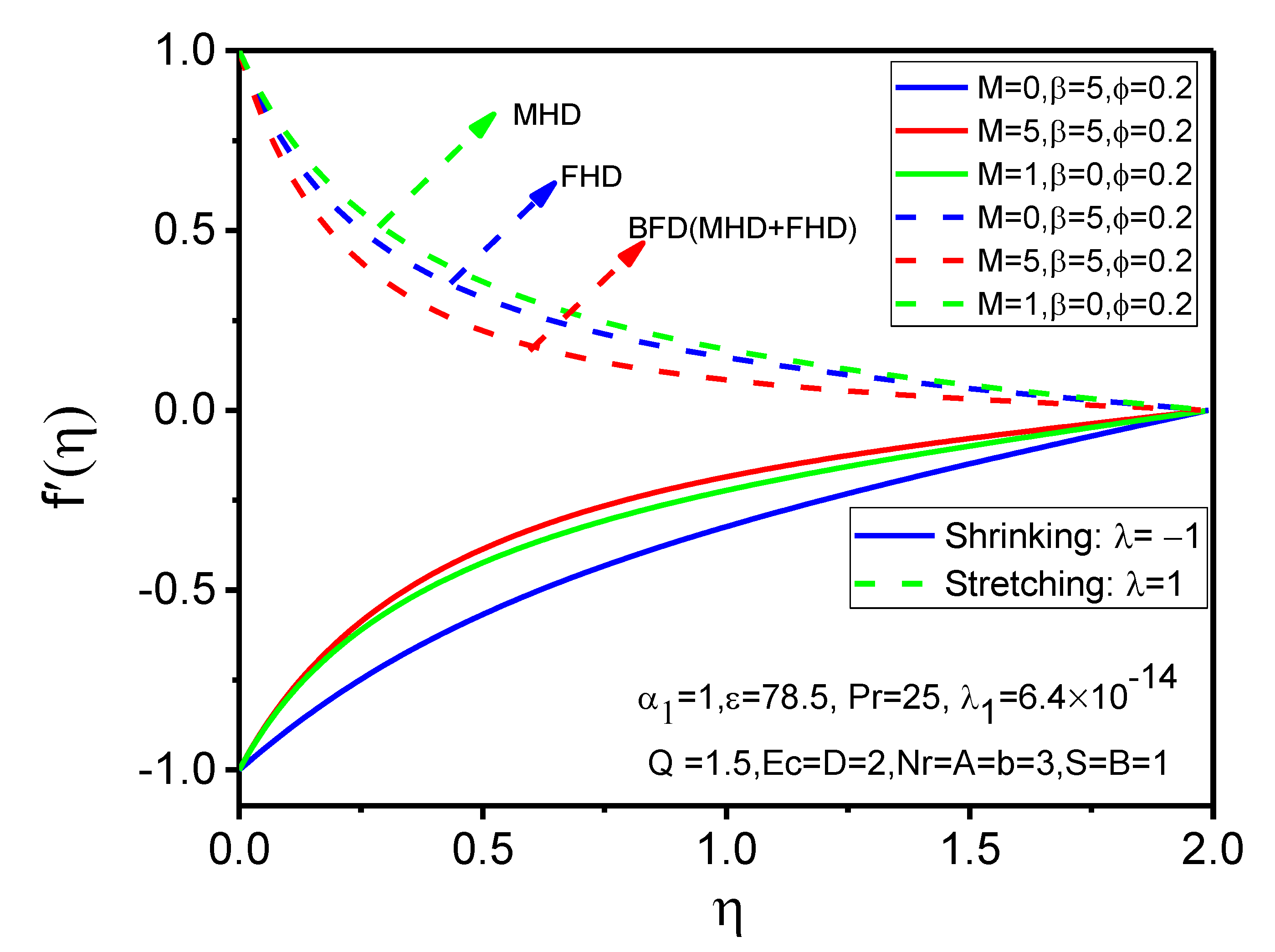
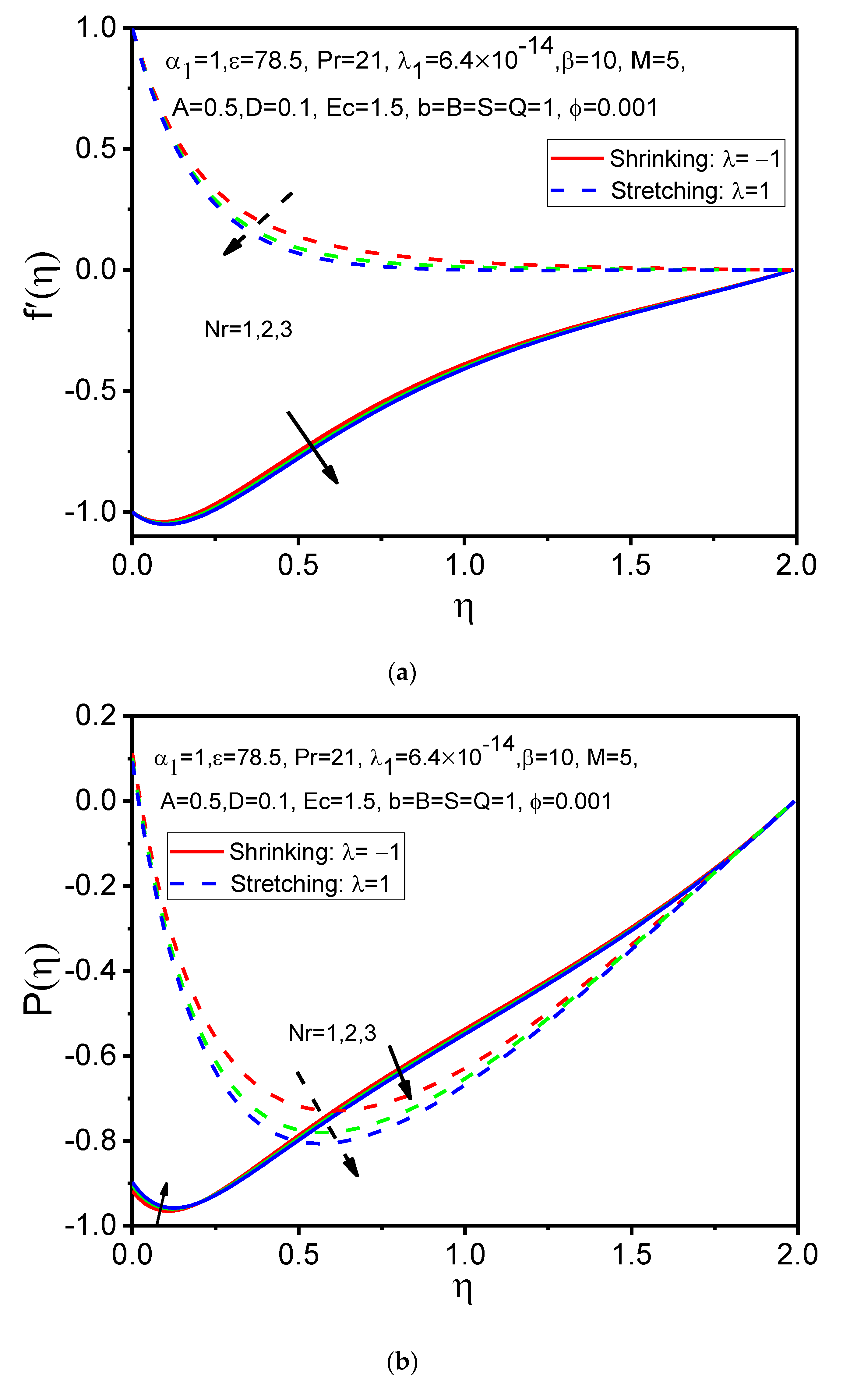
• The velocity and pressure profiles of blood-CoFe₂O₄ are decreased for both stretching and shrinking cases with the enhancement of the values of ferromagnetic interaction parameter, thermal conductivity parameter and radiation parameter.
• Increasing values of curvature parameter, volume fraction of magnetic particles and/or heat source are causing a rise in the velocity profile.
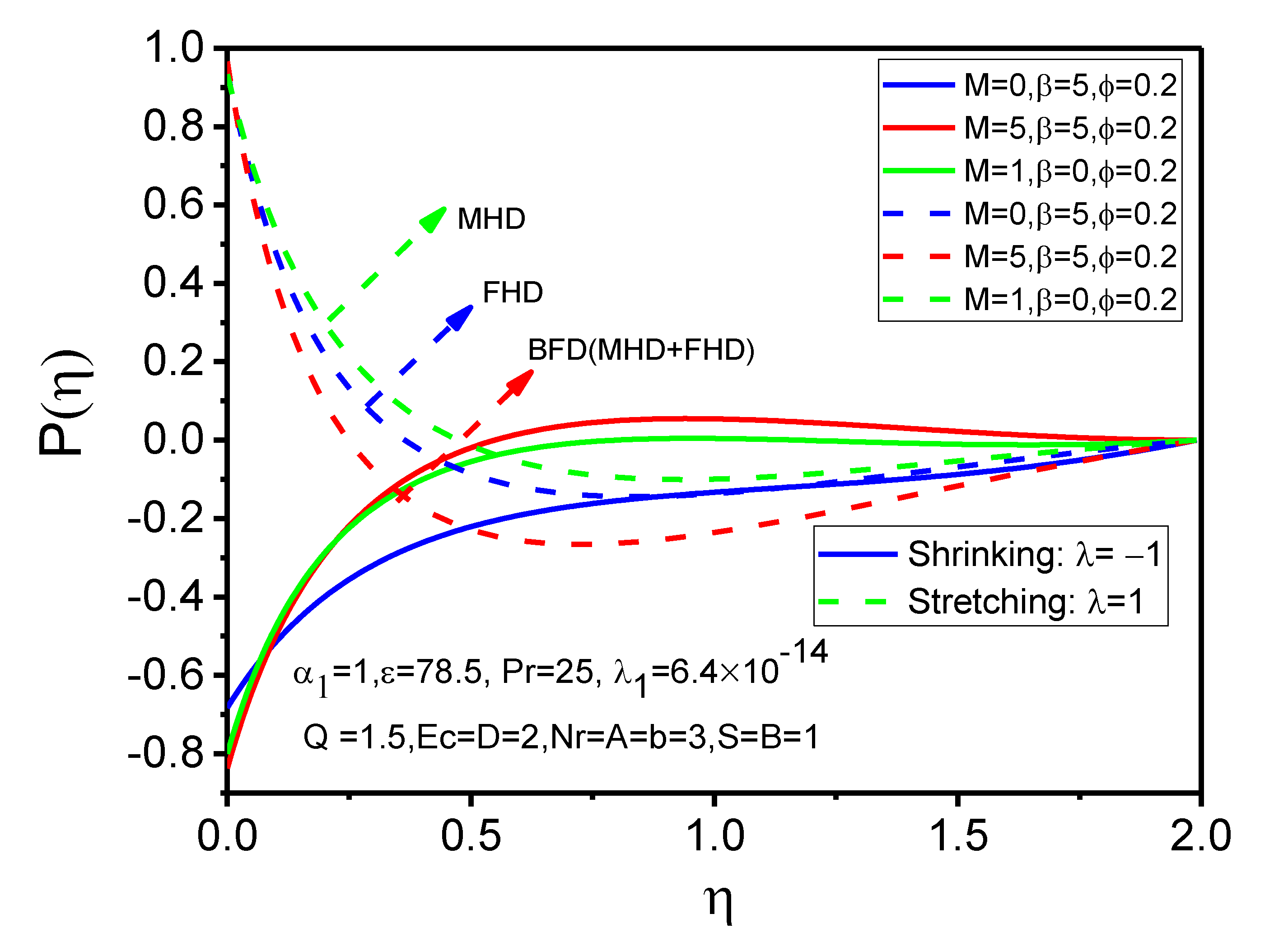
• The velocity profile is reduced when the values of the magnetic parameter and unsteady parameter are increased gradually for the stretching case, whereas the opposite behavior is observed for the shrinking case. Similar behavior is also observed for the pressure profile.
• The blood pressure is enhanced for larger values of the curvature parameter and volume fraction for the stretching case, whereas the opposite is true for the shrinking case.
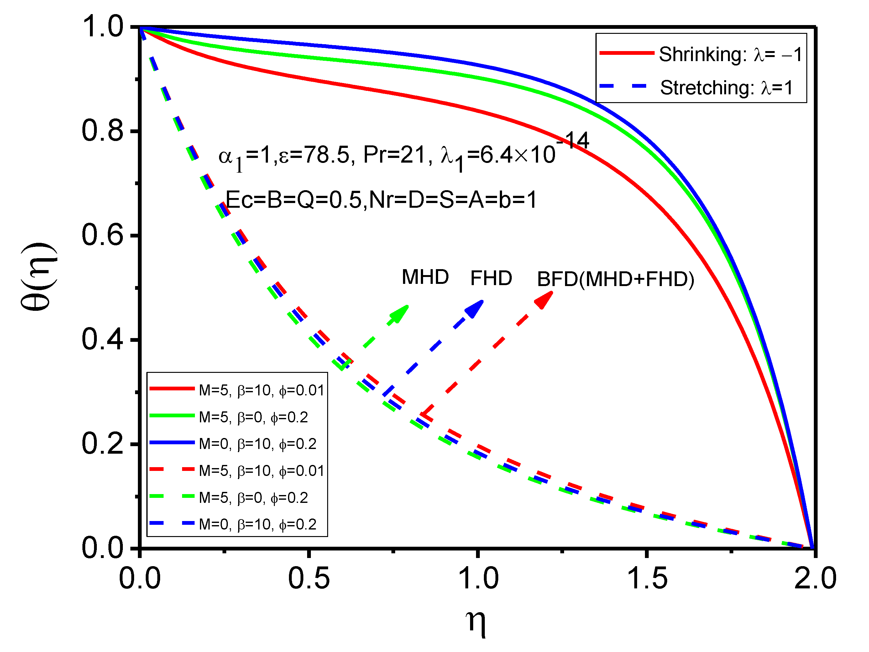
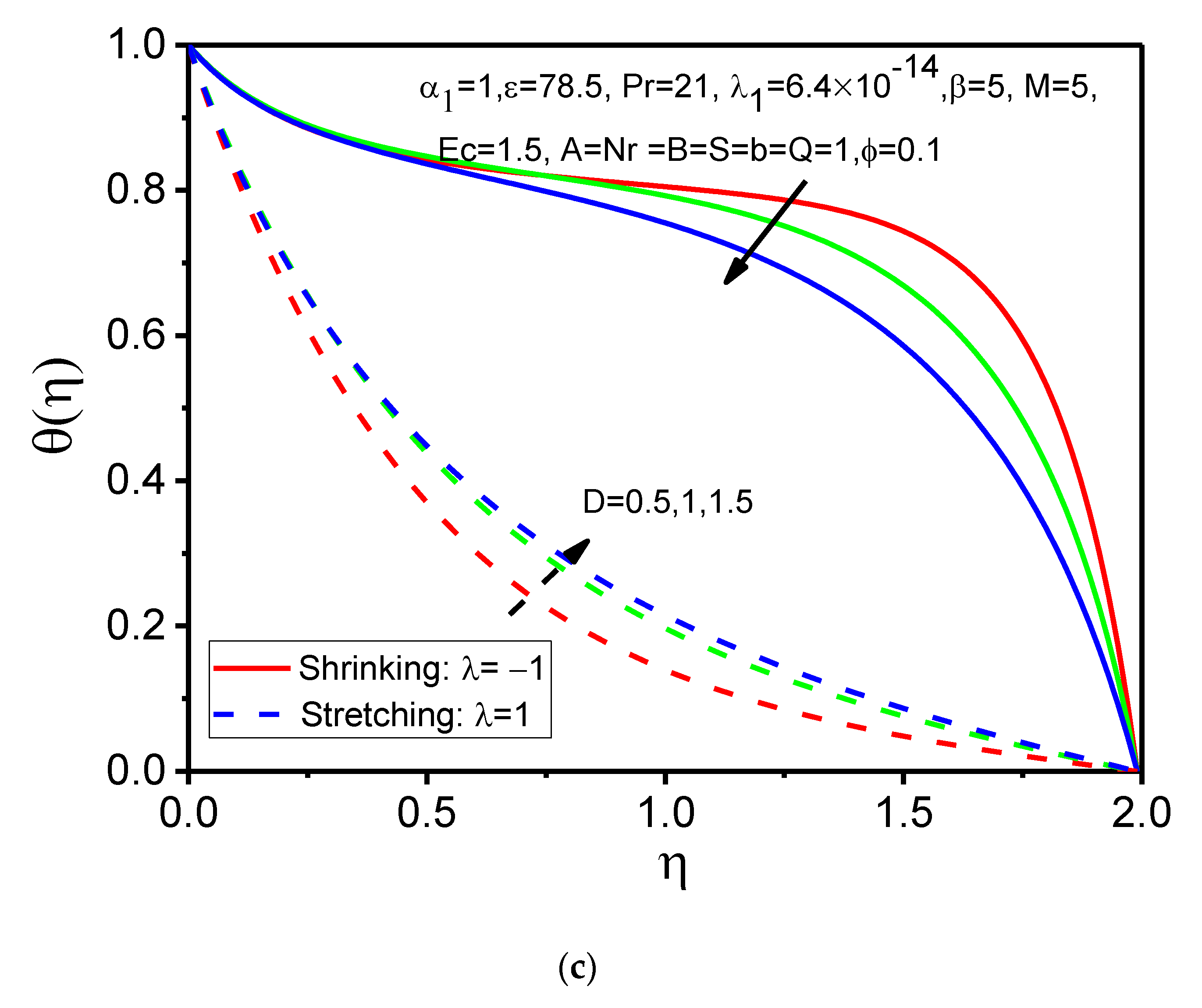
• For both stretching and shrinking cases the temperature profile exacerbates when the values of the unsteady parameter, radiation parameter and thermal conductivity parameter are increased; while the contrary behavior is found for the heat source parameter.
• With increasing values of ferromagnetic interaction parameter, magnetic field parameter, curvature parameter and the temperature profile are increased for the stretching cylinder while they are decreased in the cylinder surface for the shrinking mode.
• It is obtained temperature profile diminution with the volume fraction of the nanoparticles for the stretching mode, whereas it is raised for the shrinking case.
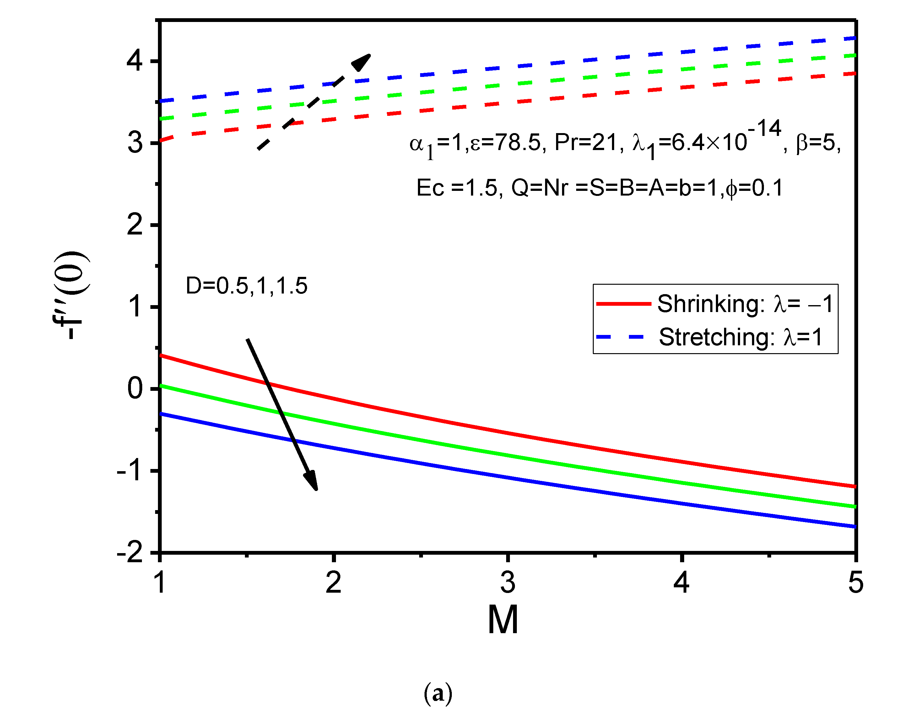
• The skin friction coefficient onward in stretching mode while it is decreased for the shrinking mode when the values of magnetic field parameter, curvature parameter and unsteady parameter are large.
• For increasing values of the ferromagnetic interaction parameter, the skin friction coefficient is enhanced for both cases, while the reverse is observed for the values of the magnetic particles volume fraction.
• The rate of heat transfer is diminished for both stretching and shrinking cases due to the enhancing values of the unsteady parameter while, interestingly, the reverse attitude is observed for the curvature parameter, magnetic field parameter and volume fraction.
• The rate of heat transfer is increased with increasing values of the ferromagnetic number as in the stretching case while the opposing trend is found for the shrinking case.

References

1. Stark, D.D.; Weissleder, R.; Elizondo, G.; Hahn, P.F.; Saini, S.; Todd, L.E.; Wittenberg, J.; Ferrucci, J.T. Superparamagnetic iron oxide: Clinical application as a contrast agent for MR imaging of the liver. Radiology 1988, 168, 297–301. [Google Scholar] [CrossRef] [PubMed]
2. Lu, J.; Ma, S.; Sun, J.; Xia, C.; Liu, C.; Wang, Z. Magnetese ferrite nanoparticle micellarnanocomposites as MRI contrast agent for liver imaging. Biomaterials 2009, 30, 2919–2928. [Google Scholar] [CrossRef]
3. Suzuki, M.; Honda, H.; Kobayashi, T.; Wakabayashi, T.; Yoshida, J.; Takahashi, M. Development of a target-directed magnetic resonance contrast agent using monoclonal antibody-conjugated magnetic particles. Brain Tumor Pathol. 1996, 13, 127–132. [Google Scholar]
4. Dürr, S.; Janko, C.; Lyer, S.; Tripal, P.; Schwarz, M.; Zaloga, J.; Tietze, R.; Alexiou, C. Magnetic nanoparticles for cancer therapy. Nanotechnol. Rev. 2013, 2, 395–409. [Google Scholar] [CrossRef] [Green Version]
5. Haik, Y.; Chen, J.C.; Pai, V.M. Development of bio-magnetic fluid dynamics. In Proceedings of the IX International Symposium on Transport Properties in Thermal Fluids Engineering, Singapore, 25–28 June 1996; Winoto, S.H., Chew, Y.T., Wijeysundera, N.E., Eds.; Pacific Center of Thermal Fluid Engineering: Kihei, HI, USA, 1996; pp. 121–126. [Google Scholar]
6. Tzirtzilakis, E.E. A mathematical model for blood flow in magnetic field. Phys. Fluids 2005, 17, 077103. [Google Scholar] [CrossRef]
7. Tzirtzilakis, E.E. Biomagnetic fluid flow in an aneurysm using ferrohydrodynamics principles. Phys. Fluids 2015, 27, 061902. [Google Scholar] [CrossRef]
8. Abdollahzadeh Jamalobadi, M.Y.; Daqiqshirazij, M.; Nasir, H.; Safaei, M.R.; Nguyen, T.K. Modeling and analysis of biomagnetic blood carreau fluid flow through a stenosis artery with magnetic heat transfer: A transient study. PLoS ONE 2018, 13, e0192138. [Google Scholar] [CrossRef]
9. Murtaza, M.G.; Tzirtzilakis, E.E.; Ferdows, M. Three-Dimensional Biomagnetic Flow and Heat Transfer over a Stretching Surface with Variable Fluid Properties. Adv. Mech. Math. 2019, 3, 403–414. [Google Scholar]
10. Murtaza, M.G.; Tzirtzilakis, E.E.; Ferdows, M. Effect of electrical conductivity and magnetization on the biomagnetic fluid flow over a stretching sheet. Z. Angew. Phys. 2017, 68, 93. [Google Scholar] [CrossRef]
11. Murtaza, M.G.; Tzirtzilakis, E.E.; Ferdows, M. Numerical solution of three dimensional unsteady biomagnetic flow and heat transfer through stretching/shrinking sheet using temperature dependent magnetization. Arch. Mech. 2018, 70, 161–185. [Google Scholar]
12. Misra, J.C.; Shit, G.C. Flow of a Biomagnetic Visco-Elastic Fluid in a Channel with Stretching Walls. J. Appl. Mech. 2009, 76, 061006. [Google Scholar] [CrossRef]
13. Misra, J.C.; Sinha, A. Effect of thermal radiation on MHD flow of blood and heat transfer in a permeable capillary in stretching motion. Heat Mass Transf. 2013, 49, 617–628. [Google Scholar] [CrossRef] [Green Version]
14. Misra, J.C.; Sinha, A.; Shit, G.C. Flow of a biomagnetic viscoelastic fluid: Application to estimation of blood flow in arteries during electromagnetic hyperthermia, a therapeutic procedure for cancer treatment. Appl. Math. Mech. 2010, 31, 1405–1420. [Google Scholar] [CrossRef]
15. Sushma, S.; Samuel, N.; Neeraja, G. Slip flow effects on unsteady MHD blood flow in a permeable vessel in the presence of heat source/sink and chemical reaction. Glob. J. Pure Appl. Math. 2018, 14, 1083–1099. [Google Scholar]
16. Ferdows, M.; Murtaza, M.G.; Tzirtzilakis, E.E.; Alzahrani, F. Numerical study of blood flow and heat transfer through stretching cylinder in the presence of a magnetic dipole. Z. Angew. Math. Mech. 2020, 100, e201900278. [Google Scholar] [CrossRef]
17. Choi, S.U.S.; Eastman, J.A. Enhancing thermal conductivity of fluids with nanoparticles. In Proceedings of the ASME International Mechanical Engineering Congress & Exposition, San Francisco, CA, USA, 12–17 November 1995; pp. 99–105. [Google Scholar]
18. Pak, B.C.; Cho, Y.I. Hydrodynamic and heat transfer study of dispersed fluids with submicron metallic oxide. Exp. Heat Transf. 1998, 11, 151–170. [Google Scholar] [CrossRef]
19. Qasim, M.; Khan, Z.H.; Khan, W.; Shah, I.A. MHD Boundary Layer Slip Flow and Heat Transfer of Ferrofluid along a Stretching Cylinder with Prescribed Heat Flux. PLoS ONE 2014, 9, e83930. [Google Scholar] [CrossRef]
20. Singh, K.; Pandey, A.K.; Kumar, M. Melting heat transfer assessment on magnetic nanofluid flow past a porous stretching cylinder. J. Egypt. Math. Soc. 2021, 29, 1. [Google Scholar] [CrossRef]
21. Malik, R.; Khan, M.; Mushtaq, M. Cattaneo-Christov heat flux model for Sisko fluid flow past a permeable non-linearly stretching cylinder. J. Mol. Liq. 2016, 222, 430–434. [Google Scholar] [CrossRef]
22. Abbas, Z.; Rasool, S.; Rashidi, M.M. Heat transfer analysis due to an unsteady stretching/shrinking cylinder with partial slip condition and suction. Ain Shams Eng. J. 2015, 6, 939–945. [Google Scholar] [CrossRef] [Green Version]
23. Islam, S.; Khan, A.; Kumam, P.; Alrabaiah, H.; Shah, Z.; Khan, W.; Zubair, M.; Jawad, M. Radiative mixed convection flow of maxwell nanofluid over a stretching cylinder with joule heating and heat source/sink effects. Sci. Rep. 2020, 10, 17823. [Google Scholar] [CrossRef] [PubMed]
24. Salahuddin, T.; Hussain, A.; Malik, M.Y.; Awais, M.; Khan, M. Carreau nanofluid impinging over a stretching cylinder with generalized slip effects: Using finite difference scheme. Results Phys. 2017, 7, 3090–3099. [Google Scholar] [CrossRef]
25. Zeeshan, A.; Maskeen, M.M.; Mehmood, O.U. Hydromagnetic nanofluid flow past a stretching cylinder embedded in non-Darcian Forchheimer porous media. Neural Comput. Appl. 2018, 30, 3479–3489. [Google Scholar] [CrossRef]
26. Ashorynejad, H.R.; Sheikholeslami, M.; Pop, I.; Ganji, D.D. Nanofluid flow and heat transfer due to a stretching cylinder in the presence of magnetic field. Heat Mass Transf. 2013, 49, 427–436. [Google Scholar] [CrossRef]
27. Gangadhar, K.; Venkata, R.; Dasaradha, R.; Kamar, B.R. Slip flow of a nanofluid over a stretching cylinder with Cattaneo-Christov flux model: Using SRM. Int. J. Eng. Technol. 2018, 7, 225–232. [Google Scholar]
28. Kakac, K.; Pramuanjaroenkij, A. Review of convective heat transfer enhancement with nanofluids. Int. J. Heat Mass Transf. 2009, 52, 3187–3196. [Google Scholar] [CrossRef]
29. Kleinstreuer, C.; Feng, Y. Experimental and theoretical studies of nanofluid thermal conductivity enhancement: A review. Nanoscale Res. Lett. 2011, 6, 229. [Google Scholar] [CrossRef] [Green Version]
30. Ozernic, S.; Kakac, S.; Yazcioglu, A. Enhanced thermal conductivity of nanofluids: A state of the art-review. Renew. Sustain. Energy Rev. 2010, 25, 670–686. [Google Scholar]
31. Khan, S.U.; Al-Khaled, K.; Aldabesh, A.; Awais, M.; Tlili, I. Bioconvection flow in accelerated couple stress nanoparticles with activation energy: Bio-fuel applications. Sci. Rep. 2021, 11, 3331. [Google Scholar] [CrossRef]
32. Kolsi, L.; Dero, S.; Ali-Lund, L.; Alqsair, U.F.; Omri, M.; Khan, S.U. Thermal stability and performances of hybrid nanoparticles for convective heat transfer phenomenon with multiple solutions. Case Stud. Therm. Eng. 2021, 28, 101684. [Google Scholar] [CrossRef]
33. Abbasi, A.; Khan, S.U.; Al-Khaled, K.; Khan, M.I.; Farooq, W.; Galal, A.M.; Javid, K.; Malik, M. Thermal prospective of Casson nano-materials in radiative binary reactive flow near oblique stagnation point flow with activation energy applications. Chem. Phys. Lett. 2021, 786, 139172. [Google Scholar] [CrossRef]
34. Islam, S.; Dawar, A.; Shah, Z.; Tariq, A. Cattaneo–Christov theory for a time-dependent magnetohydrodynamic Maxwell fluid flow through a stretching cylinder. Adv. Mech. Eng. 2021, 13, 1–11. [Google Scholar] [CrossRef]
35. Krishnamurthy, M.; Prasannakumara, B.; Gireesha, B.; Gorla, R.S.R. Effect of chemical reaction on MHD boundary layer flow and melting heat transfer of Williamson nanofluid in porous medium. Eng. Sci. Technol. Int. J. 2016, 19, 53–61. [Google Scholar] [CrossRef] [Green Version]
36. Rosensweig, R.E. Magnetic fluids. Annu. Rev. Fluid Mech. 1987, 19, 437–461. [Google Scholar] [CrossRef]
37. Das, S.; Chakraborty, S.; Jana, R.N.; Makinde, O.D. Entropy analysis of unsteady magneto-nanofluid flow past accelerating stretching sheet with convective boundary condition. Appl. Math. Mech. 2015, 36, 1593–1610. [Google Scholar] [CrossRef]
38. Dandapat, B.S.; Santra, B.; Singh, S.K. Thin film flow over a non-linear stretching sheet in presence of uniform transverse magnetic field. Z. Angew. Math. Phys. 2010, 61, 685–695. [Google Scholar] [CrossRef]
39. Misra, J.C.; Rath, H.J.; Shit, G.C. Flow and heat transfer of a MHD viscoelastic fluid in a channel with stretching walls: Some applications to haemodynamics. Comput. Fluids 2008, 37, 1–11. [Google Scholar] [CrossRef] [Green Version]
40. Tzirtzilakis, E.; Kafoussias, N.G. Three-Dimensional Magnetic Fluid Boundary Layer Flow over a Linearly Stretching Sheet. J. Heat Transf. 2009, 132, 1–8. [Google Scholar] [CrossRef]
41. Tzirtzilakis, E.E.; Kafoussias, N.G. Biomagnetic fluid flow over a stretching sheet with nonlinear temperature dependent magnetization. Z. Angew. Math. Phys. 2003, 54, 551–565. [Google Scholar]
42. Tzirtzilakis, E.; Tanoudis, G. Numerical study of biomagnetic fluid flow over a stretching sheet with heat transfer. Int. J. Numer. Methods Heat Fluid Flow 2003, 13, 830–848. [Google Scholar] [CrossRef] [Green Version]
43. Nadeem, S.; Ullah, N.; Khan, A.U.; Akbar, T. Effect of homogeneous-heterogeneous reactions on ferrofluid in the presence of magnetic dipole along a stretching cylinder. Results Phys. 2017, 7, 3574–3582. [Google Scholar] [CrossRef]
44. Tahir, H.; Khan, U.; Din, A.; Chu, Y.-M.; Muhammad, N. Heat Transfer in a Ferromagnetic Chemically Reactive Species. J. Thermophys. Heat Transf. 2021, 35, 402–410. [Google Scholar] [CrossRef]
45. Makinde, O.D. Stagnation Point flow with heat and mass transfer and temporal stability of ferrofluid past a permeable stretching/shrinking sheet. Defect Diffus. Forum 2018, 387, 510–522. [Google Scholar] [CrossRef]
46. Alam, J.; Murtaza, G.; Tzirtzilakis, E.; Ferdows, M. Biomagnetic Fluid Flow and Heat Transfer Study of Blood with Gold Nanoparticles over a Stretching Sheet in the Presence of Magnetic Dipole. Fluids 2021, 6, 113. [Google Scholar] [CrossRef]
47. Kafoussias, N.G.; Williams, E.W. An improved approximation technique to obtain numerical solution of a class of two-point boundary value similarity problems in fluid mechanics. Int. J. Numer. Methods Fluids 1993, 17, 145–162. [Google Scholar] [CrossRef]
48. Vajravelu, K.; Prasad, K.; Santhi, S. Axisymmetric magneto-hydrodynamic (MHD) flow and heat transfer at a non-isothermal stretching cylinder. Appl. Math. Comput. 2012, 219, 3993–4005. [Google Scholar] [CrossRef] [Green Version]
49. Bhattacharyya, K.; Gorla, R. Boundary layer flow and heat transfer over a permeable shrinking cylinder with surface mass transfer. Int. J. Appl. Mech. Eng. 2013, 18, 1003–1012. [Google Scholar] [CrossRef] [Green Version]
50. Tzirtzilakis, E.E.; Xenos, M.; Loukopoulos, V.C.; Kafoussias, N.G. Turbulent biomagnetic fluid flow in a rectangular channel under the action of a localized magnetic field. Int. J. Eng. Sci. 2006, 44, 1205–1224. [Google Scholar] [CrossRef]
51. Alam, M.J.; Murtaza, M.G.; Tzirtzilakis, E.E.; Ferdows, M. Effect of thermal radiation on biomagnetic fluid flow and heat transfer over an unsteady stretching sheet. Comput. Assist. Methods Eng. Sci. (CAMES) 2021, 28, 81–104. [Google Scholar]
52. Bhattacharyya, K. Effects of heat source/sink on MHD flow and heat transfer over a shrinking sheet with mass suction. Chem. Eng. Res. Bull. 2011, 15, 12–17. [Google Scholar] [CrossRef]
53. Ismail, H.N.; Abdel-Wahed, M.S.; Omama, M. Effect of variable thermal conductivity on the MHD boundary-layer of Casson nanofluid over a moving plate with variable thickness. Therm. Sci. 2021, 25, 145–157. [Google Scholar] [CrossRef]
54. Muhammad, K.A.M.; Farah, N.A.; Salleh, M.Z. MHD boundary layer flow over a permeable flat plate in a ferrofluid with thermal radiation effect. J. Phys. Conf. Ser. 2019, 1366, 012014. [Google Scholar]
55. Kumar, K.A.; Sandeep, N.; Sugunamma, V.; Animasaum, I.I. Effect of irregular heat source/sink on the radiative thin film flow of MHD hybrid ferrofluid. J. Therm. Anal. 2020, 139, 2145–2153. [Google Scholar] [CrossRef]
56. Ferdows, M.; Murtaza, G.; Misra, J.C.; Tzirtzilakis, E.E.; Alsenafi, A. Dual solutions in biomagnetic fluid flow and heat transfer over a nonlinear stretching/shrinking sheet: Application of lie group transformation method. Math. Biosci. Eng. 2020, 17, 4852–4874. [Google Scholar] [CrossRef] [PubMed]
Figure 1. Graphical representation and coordinate system of given flow problem (a) for stretching cylinder and (b) for shrinking cylinder.
Magnetochemistry 08 00027 g001
Figure 2. Velocity profile for BFD, MHD and FHD.
Magnetochemistry 08 00027 g002
Figure 3. Pressure profile for BFD, MHD and FHD.
Magnetochemistry 08 00027 g003
Figure 4. Temperature profile for BFD, MHD and FHD.
Magnetochemistry 08 00027 g004
Figure 5. Variation of β on (a) velocity profile, (b) Pressure profile, (c) Temperature profile.
Magnetochemistry 08 00027 g005aMagnetochemistry 08 00027 g005b
Figure 6. Variation of M on (a) Velocity profile, (b) Pressure profile, (c) Temperature profile.
Magnetochemistry 08 00027 g006aMagnetochemistry 08 00027 g006b
Figure 7. Variation of D on (a) Velocity profile, (b) Pressure profile, (c) Temperature profile.
Magnetochemistry 08 00027 g007aMagnetochemistry 08 00027 g007b
Figure 8. Variation of ϕ on (a) Velocity profile, (b) Pressure profile, (c) Temperature profile.
Magnetochemistry 08 00027 g008aMagnetochemistry 08 00027 g008b
Figure 9. Variation of A on (a) Velocity profile, (b) Pressure profile, (c) Temperature profile.
Magnetochemistry 08 00027 g009aMagnetochemistry 08 00027 g009b
Figure 10. Variation of b on (a) Velocity profile, (b) Pressure profile, (c) Temperature profile.
Magnetochemistry 08 00027 g010aMagnetochemistry 08 00027 g010b
Figure 11. Variation of N r on (a) Velocity profile, (b) Pressure profile, (c) Temperature profile.
Magnetochemistry 08 00027 g011aMagnetochemistry 08 00027 g011b
Figure 12. Variation of Q on (a) Velocity profile, (b) Pressure profile, (c) Temperature profile.
Magnetochemistry 08 00027 g012aMagnetochemistry 08 00027 g012b
Figure 13. Influence of β against M on (a) Skin friction coefficient, (b) Rate of heat transfer.
Magnetochemistry 08 00027 g013aMagnetochemistry 08 00027 g013b
Figure 14. Influence of D against M on (a) Skin friction coefficient, (b) Rate of heat transfer.
Magnetochemistry 08 00027 g014aMagnetochemistry 08 00027 g014b
Figure 15. Influence of M against β on (a) Skin friction coefficient, (b) Rate of heat transfer.
Magnetochemistry 08 00027 g015aMagnetochemistry 08 00027 g015b
Figure 16. Influence of φ against β on (a) Skin friction coefficient, (b) Rate of heat transfer.
Magnetochemistry 08 00027 g016aMagnetochemistry 08 00027 g016b
Figure 17. Influence of A against β on (a) Skin friction coefficient, (b) Rate of heat transfer.
Magnetochemistry 08 00027 g017aMagnetochemistry 08 00027 g017b