Article

Deep Feature Extraction for Cymbidium Species Classification Using Global–Local CNN

Hangzhou Academy of Agricultural Sciences, Hangzhou 311400, China
*
Author to whom correspondence should be addressed.
Horticulturae 2022, 8(6), 470; https://doi.org/10.3390/horticulturae8060470
Submission received: 12 April 2022 / Accepted: 27 April 2022 / Published: 25 May 2022

Abstract

:
Cymbidium is the most famous and widely distributed type of plant in the Orchidaceae family. It has extremely high ornamental and economic value. With the continuous development of the Cymbidium industry in recent years, it has become increasingly difficult to classify, identify, develop, and utilize orchids. In this study, a classification model GL-CNN based on a convolutional neural network was proposed to solve the problem of Cymbidium classification. First, the image set was expanded by four methods (mirror rotation, salt-and-pepper noise, image sharpening, and random angle flip), and then a cascade fusion strategy was used to fit the multiscale features obtained from the two branches. Comparing the performance of GL-CNN with other four classic models (AlexNet, ResNet50, GoogleNet, and VGG16), the results showed that GL-CNN achieves the highest classification prediction accuracy with a value of 94.13%. This model can effectively detect different species of Cymbidium and provide a reference for the identification of Cymbidium germplasm resources.

1. Introduction

Orchidaceae is one of the largest and most diverse flowering plants and has been widespread all around the world [1]. Cymbidium, belonging to the Orchidaceae family, with elegant and upright leaves and fragrant flowers, is the most important and economic flowering genus. It is popular in Asia, especially in China, Japan, Korea, and Southeast Asia [2]. In China, the Cymbidium has more than a thousand years of history with extremely high cultural and economic value [3]. The flowers of Cymbidium have various colors and shape patterns, which usually leads to confusion when comparing cultivars to assess genetic resources at the species level [4]. In recent years, with the continuous development of the Cymbidium industry, the number of Cymbidium germplasm resources has increased year by year, which greatly increases the difficulty of orchid classification, identification, and development. Traditional approaches for the classification of Cymbidium cultivars are based on morphological traits, which are difficult due to the problems associated with morphological variability, growth conditions, overlapping geographical origins, and individual biases, and most of these cultivars are related [5,6,7]. It requires professionals but offers jugged with subjective. Molecular recognition is the most effective method to identify the various Cymbidium cultivars [8,9,10], but often time and cost-consuming, making it unsuitable for high throughput and rapid classification.
Recently, an emerging field of machine learning, deep learning (DL), known as deep neural networks, has been growing fast and widely used in many fields, such as image processing, content prediction, and text understanding [11]. The main core of the deep learning algorithm is largely inherited from artificial neural network architecture with many hidden layers. Deep learning allows computers to process and analyze images and extract image details similar to the human brain and has been significantly progressed for image pattern recognition as computer vision algorithms [12]. Convolutional neural network (CNN) is one of the most common methods for visual image classification and has been widely adopted by the research community [13]. With the support of powerful graphics processing units (GPU), CNN can be easily used with low-cost normal image data and huge numbers of datasets, as deep learning often requires large datasets and powerful resources for model training [14]. Inspired by the results of image classification and object detection, many researchers use CNN to identify plant images [15,16]. For instance, CNN has been successfully used to automatically learn discriminative features from leaf images [17] and to detect the diversity in flower images [18]. In addition, the features extracted by CNN could highly improve classification accuracy and have been suggested to be the optimal candidate for any visual task [19,20]. CNN has been successfully used to extract features for hyperspectral image (HSI) classification and perform at high accuracy [21]. Hiary et al. [22] conducted a two-step deep learning model that could automatically discover the portions of flowers and use the feature extracted from this portion to yield a high classification accuracy of 97.1% on flowers. Dias et al. [23] also performed feature extraction from a fine-tuned CNN model and used these features to establish a support vector machines (SVM) classification model. The model accuracy reached 90% on apple flowers. In addition, a combination of features extracted from pretrained CNN models (AlexNet, ResNet50, and VGG-16) was also used for flower species classification, with a success rate of 80%. These pretrained models have achieved successful results in an ImageNet competition [24]. Evidence has shown that combining the feature selection of CNN model and traditional machine learning methods, such as SVM and random forest (RF), could yield a high success rate, save massive process time, and reduce computation intensity [25]. However, among the available research into CNN technologies, there is limited research into detecting flower images of diverse Cymbidium species.
CNN has a powerful ability to capture local features and keep parallel motion unchanged [26]. However, the existing classification methods based on CNN mostly focus on single-scale image datasets [27]. Global–local CNN (GL-CNN), a CNN based on multifeature fusion, can fuse global and local features. Hao et al. [27] used GL-CNN to classify the growth period of Gynura bicolor DC, and the test accuracy of GL-CNN reached 95.63%. In this study, we proposed a global–local joint training CNN framework called GL-CNN to solve the problem of identifying different Cymbidium species instead of using global image information alone. Specific objectives were to: (1) The image set was expanded by four methods (mirror rotation, salt-and-pepper noise, image sharpening, and random angle flipping) to improve the model training effect and prevent overfitting. (2) A GL-CNN architecture based on a fusion strategy was proposed to classify 10 different species of Cymbidium. (3) The GL-CNN model was compared with the four classic models (AlexNet, ResNet50, GoogleNet, and VGG16) and the model performance was comprehensively evaluated.

2. Materials and Methods

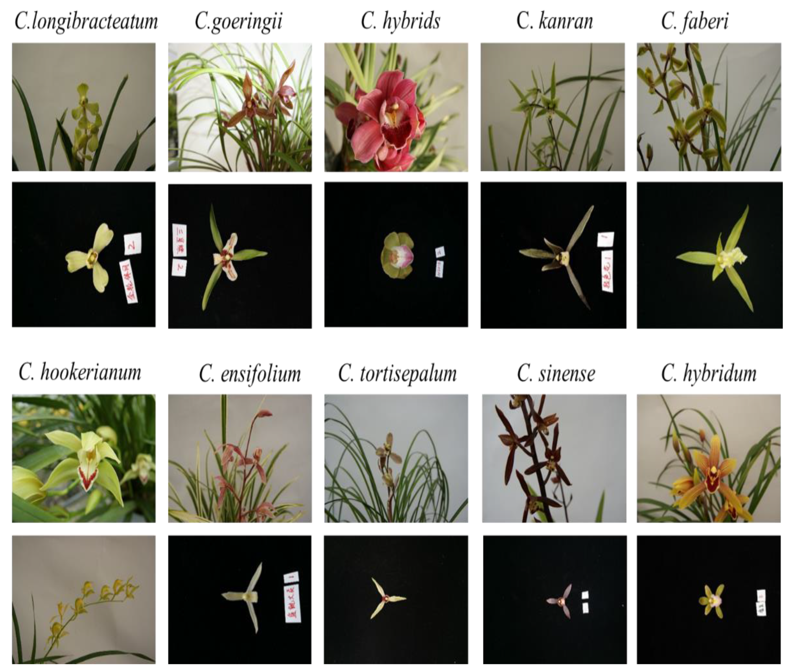
2.1. Cymbidium Species Flower Dataset

In this study, we collected 10 species of Cymbidium, which were C. goeringii, C. longibracteatum, C. faberi, C. sinense, C. hybrids, C. hybridum, C. ensifolium, C. kanran, C. hookerianum, and C. tortisepalum for flower classification. During the flowering period, the flowers of each species were pictured using a high-definition camera (Canon 500D, Tokyo, Japan). There was a total of 3390 pictures. They were divided into two types, as shown in Figure 1. One was an unpicked Cymbidium plant, and the other was a flower on a black background.

2.2. Data Preprocessing

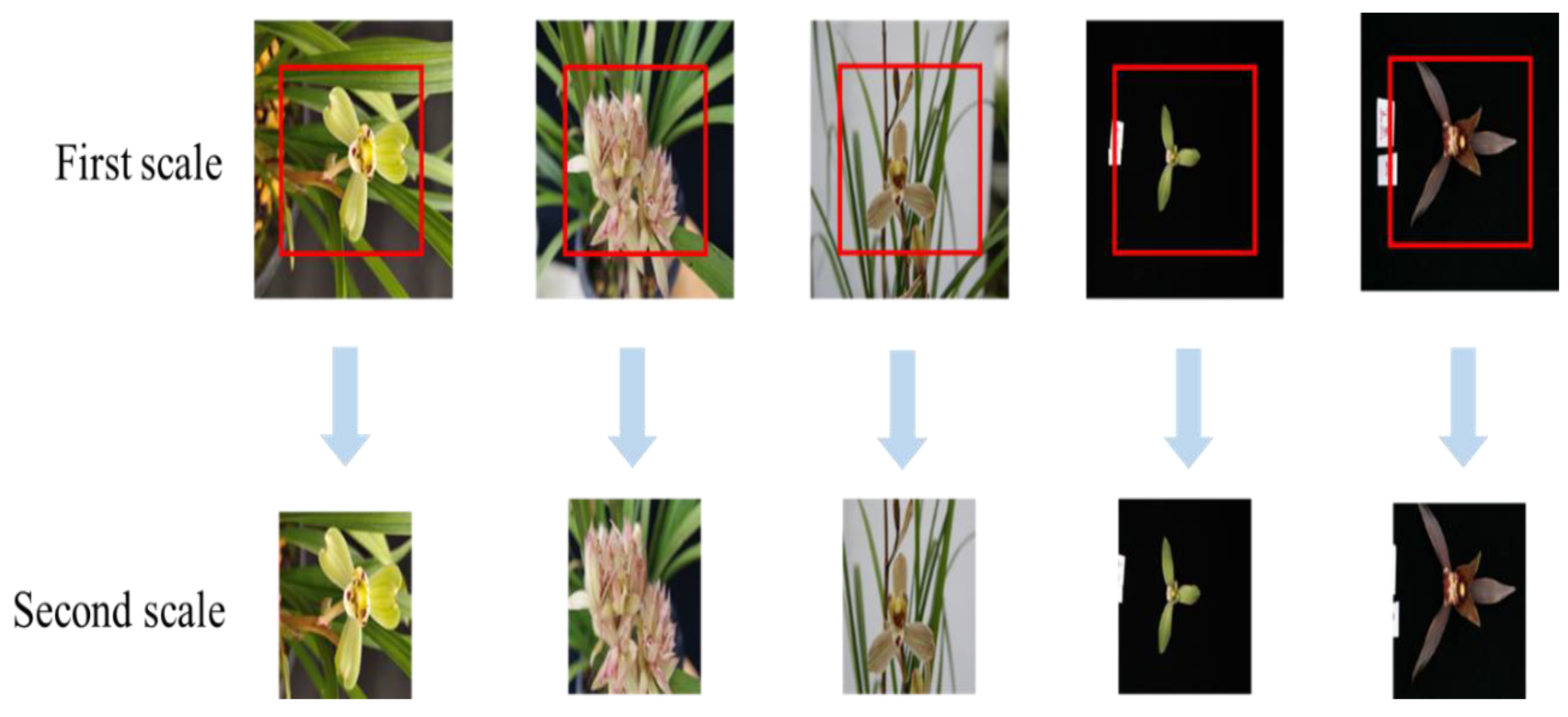
2.2.1. Two-Scale Image Acquisition

Before model training, Cymbidium images were subjected to two-scale processing to improve the robustness of the classification model established by the image with different backgrounds [27]. Figure 2 shows an image sample randomly selected from 10 Cymbidium species. The red frame represents the second scale image captured. First, set the original image to a size of 224 × 224 to obtain an image of the first scale. Since the recognition targets were basically located in the middle of the images, the experiment chose to intercept a partial image from the center of the first scale image (the height and width of the partial image were both 0.8 times of the first scale image) as the second scale image. The size of the second scale image was the same as the first scale image, which was 224 × 224 [28].

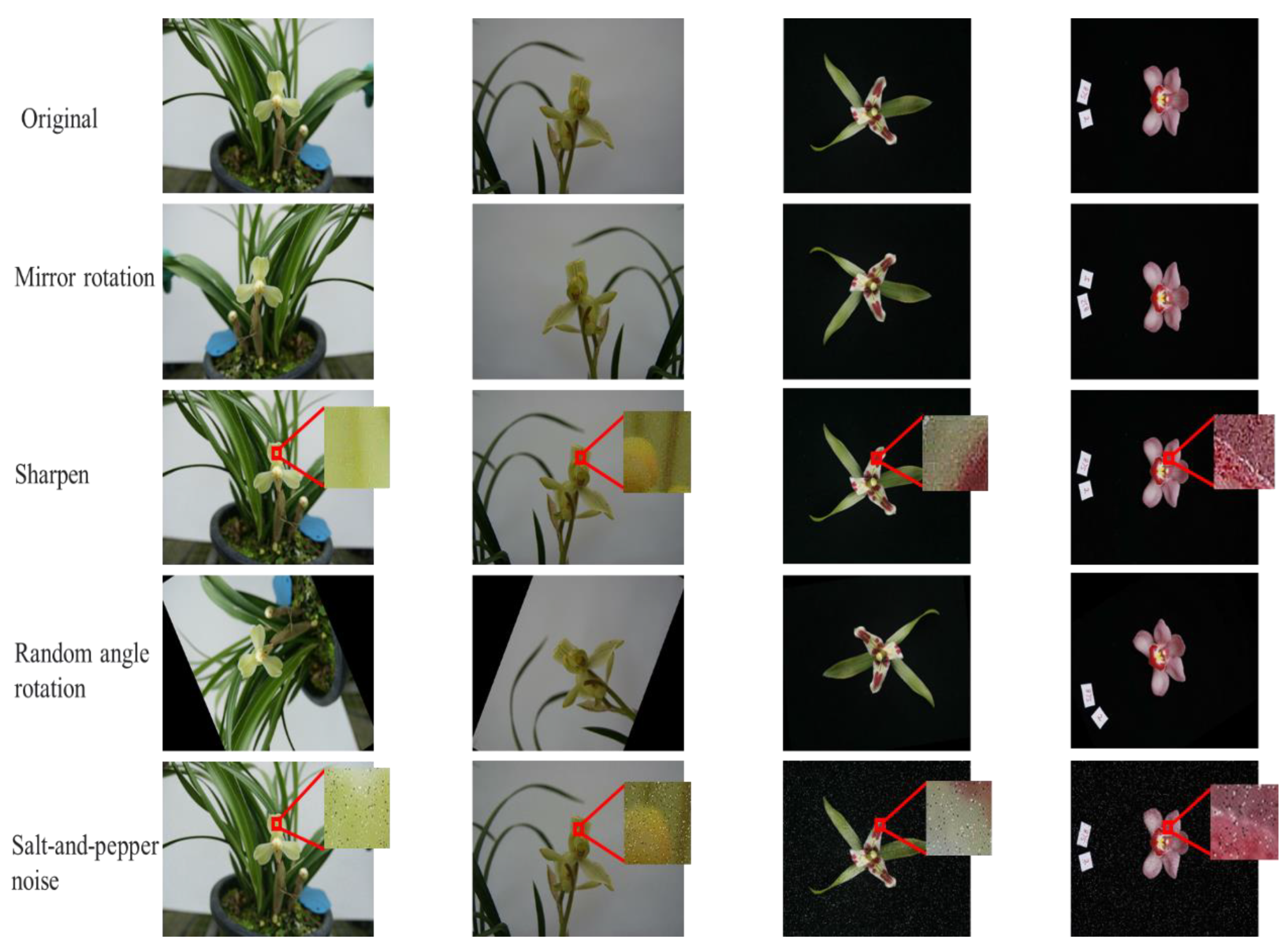
2.2.2. Data Set Enhancement

The original data set was divided into training, validation, and test sets at a ratio of 8:1:1. Although the diversity of sample species and morphology were considered in the image collection process, the growth of orchids and the imaging angle were random [26]. This experiment mainly chose mirror rotation, sharpening, salt-and-pepper noise, and random angle rotation to enhance the image set [29,30,31]. The total number of samples was expanded by four times, and the effects before and after image enhancement are shown in Figure 3.

2.3. Global–Local CNN Classification Model

2.3.1. GL-CNN Model Construction

In this part, we proposed a global–local CNN (GL-CNN) network to achieve accurate classification of different kinds of Cymbidium. The network consists of two types of features extracted from the trained GL-CNN. The first branch network is the global feature, denoted as “Gnet.” The second feature is used to capture the local information of the input image, denoted as “LNet” [27]. The overall network structure is shown in Figure 4. The model input consists of two parts. The original image is input to GNet with a size of 224 × 224, and the corresponding local images of the same size are input to LNet. There is a one-to-one correspondence between input images of two scales. This operation expands the original image information from the data level by expanding the resolution of the input image in the LNet branch.
This experiment designed different sizes of convolution kernels according to the scale of the input image in order to enhance the feature extraction ability of the network. As shown in Figure 4, since GNet extracts global features based on larger-scale images, the size of the first convolution kernel is set to 11 × 11 to extract edge features. This branch mainly includes four convolutional layers, three pooling layers, and one fully connected layer. Moreover, LNet is a detailed feature extraction branch based on a more fine-grained image design, which adds an additional convolutional layer based on GNet to abstract the features [26].

2.3.2. Cascade Fusion Strategy

We used the cascade fusion strategy to fit the multiscale features obtained from the two branches [32]. A feature fusion block was designed to capture features with more details [31]. With a cascading operation, it can process data layer-by-layer, and it only merges the two parts of the feature vectors without performing other mathematical operations. More importantly, the concatenated vector contains all the feature vectors. In a nutshell, the model can be concerned as an “ensemble of ensembles.”
In order to combine the different features of the global image and the local image, the “cascade fusion” strategy integrates FC11 and FC12 into the Cas layer through cascade (Table 1) and sends the Cas feature queue to the FC2 and FC3 layers for further feature combination and integration. Finally, the prediction probability output is realized through the SoftMax layer. The main hidden layer parameter settings are shown in Table 1.

2.3.3. Model Enhancement

The model uses ReLU6 and dropout to prevent gradient explosion and alleviate potential overfitting problems. End-to-end training is achieved through momentum stochastic gradient descent, and cross-entropy is used as the loss function.
ReLU 6 is an activation function commonly used in deep convolutional neural networks [27,33]. Relu uses x for linear activation in the region of x > 0, which may cause the value after activation to be too large and affect the stability of the model [34]. In order to offset the linear growth of the ReLU excitation function, the Relu6 function can be used. The ReLU activation function and derivative function are:
R e L U 6 ( x ) = m i n ( m a x ( x , 0 ) , 6 ) [ 0 , 6 ]
R e L U 6 ( x ) = { 1 ,     0 < x < 6 0 ,     e l s e { 0 , 1 }
Dropout is used to combat overfitting in artificial neural networks. It can avoid complicated mutual adaptation to training data [35]. During the network training process, half of the neurons are usually ignored randomly; that is, the dropout is set to 0.5. The cross-entropy loss function is used to evaluate the difference between the predicted and actual values of the model [36], which can be expressed as follows:
L = 1 N i   L i = 1 N i   c = 1 M   y i c log ( p i c )
where M is the number of categories, N is the number of samples, and y i c indicates the symbolic function (0 or 1). If the true category of the sample i is equal to C, take 1, or otherwise take 0. p i c indicates the predicted probability of the observation sample with i belonging to category C.

2.4. Model Training

2.4.1. Parameter Settings

Referring to the method of Hao et al. [27], the experiment was performed on a Windows 10 64-bit PC equipped with an Intel(R) Xeon(R) CPU @ 3.80 GHz processor, 32 GB RAM, and a GPU of NVIDIA GeForce GTX 3060. The GL-CNN model mentioned in this article is implemented based on the Keras framework. In addition, the maximum number of iterations epochs is set to 60, the initial learning rate is set to 0.05, and the learning rate is updated to 1/2 of the original value every 20 epochs. The “SGD+Momentum” strategy is adopted to update the parameters to improve the training speed of the model and avoid falling into the local optimum at the same time [37].

2.4.2. Contrast Experiment

In order to evaluate the performance of the proposed GL-CNN model in orchid-type classification tasks, comparative experiments were carried out with the classic AlexNet, ResNet50, GoogleNet, and VGG16 models. AlexNet is a convolutional neural network designed by Alex Krizhevsky and contains an eight-layer network [38]. The first five layers are convolutional layers, some of the later layers are maximum pooling layers, and the last three layers are fully connected layers. It uses a non-saturated ReLU activation function and shows better training performance than tanh and sigmoid [39]. The Residual Neural Network (ResNet) is an artificial neural network (ANN) that stacks residual blocks on top of each other to form a network. ResNet-50 is a convolutional neural network with a depth of 50 layers, which can accurately analyze visual images [40]. GoogLeNet is a type of convolutional neural network based on the Inception architecture [39]. It utilizes Inception modules, which allow the network to choose between multiple convolutional filter sizes in each block. An Inception network stacks these modules on top of each other, with occasional max-pooling layers with stride 2 to halve the resolution of the grid. VGG16 is a convolutional neural network model proposed by K. Simonyan and A. Zisserman of Oxford University. This model achieves a top-five test accuracy rate of 92.7% in ImageNet [28].

2.4.3. Model Performance Evaluation

Four metrics, namely, precision, recall, F1-score, and accuracy, were used to evaluate the classification model [27,41], and the formulas are expressed as follows:
P r e c i s i o n = T P T P + F P
R e c a l l = T P T P + F N
A c c u r a c y = T P + T N T P + T N + F P + F N
F 1 = 2 T P 2 T P + F P + F N
where true positive (TP) refers to the number of samples whose predicted value and actual value are both positive. False positive (FP) refers to the number of samples whose predicted value is positive, and the actual value is negative. False negative (FN) means false negative, which refers to the number of samples whose predicted value is negative, and the measured value is positive, correspondingly. True negative (TN) is true negative, which refers to the number of samples whose predicted value and actual value are both negative.

3. Results

3.1. Data Collection and Preprocessing

In the image samples randomly selected from 10 Cymbidium species shown in Figure 2, it can be observed that the background of the second scale image was smaller, and the details of the flower such as veins and textures were more abundant, which was more helpful to expand the input features and improve the classification accuracy. Four data enhancement methods, i.e., mirror rotation, sharpening, salt-and-pepper noise, and random angle rotation, were used to expand the training set by four times to prevent overfitting.

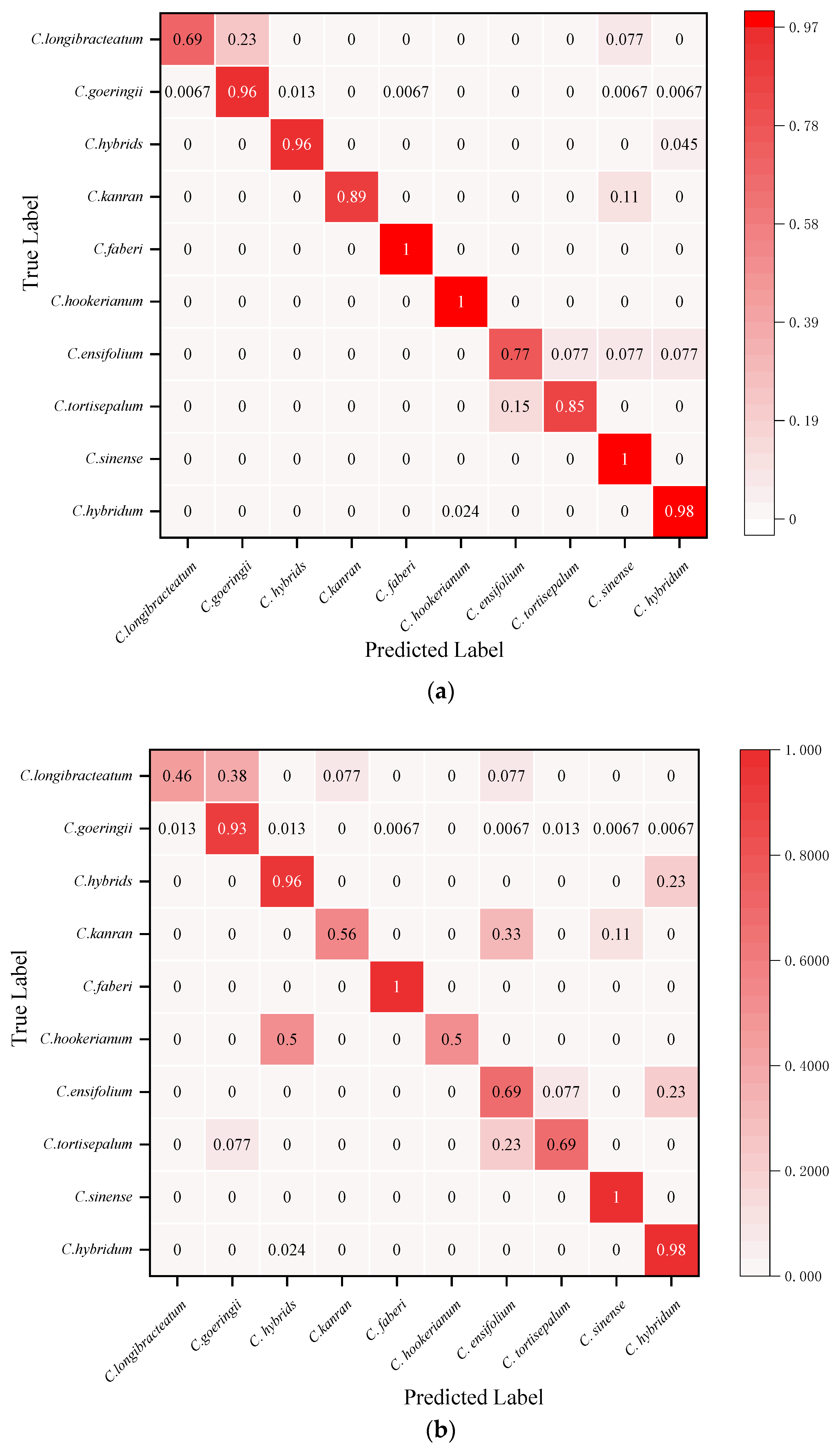
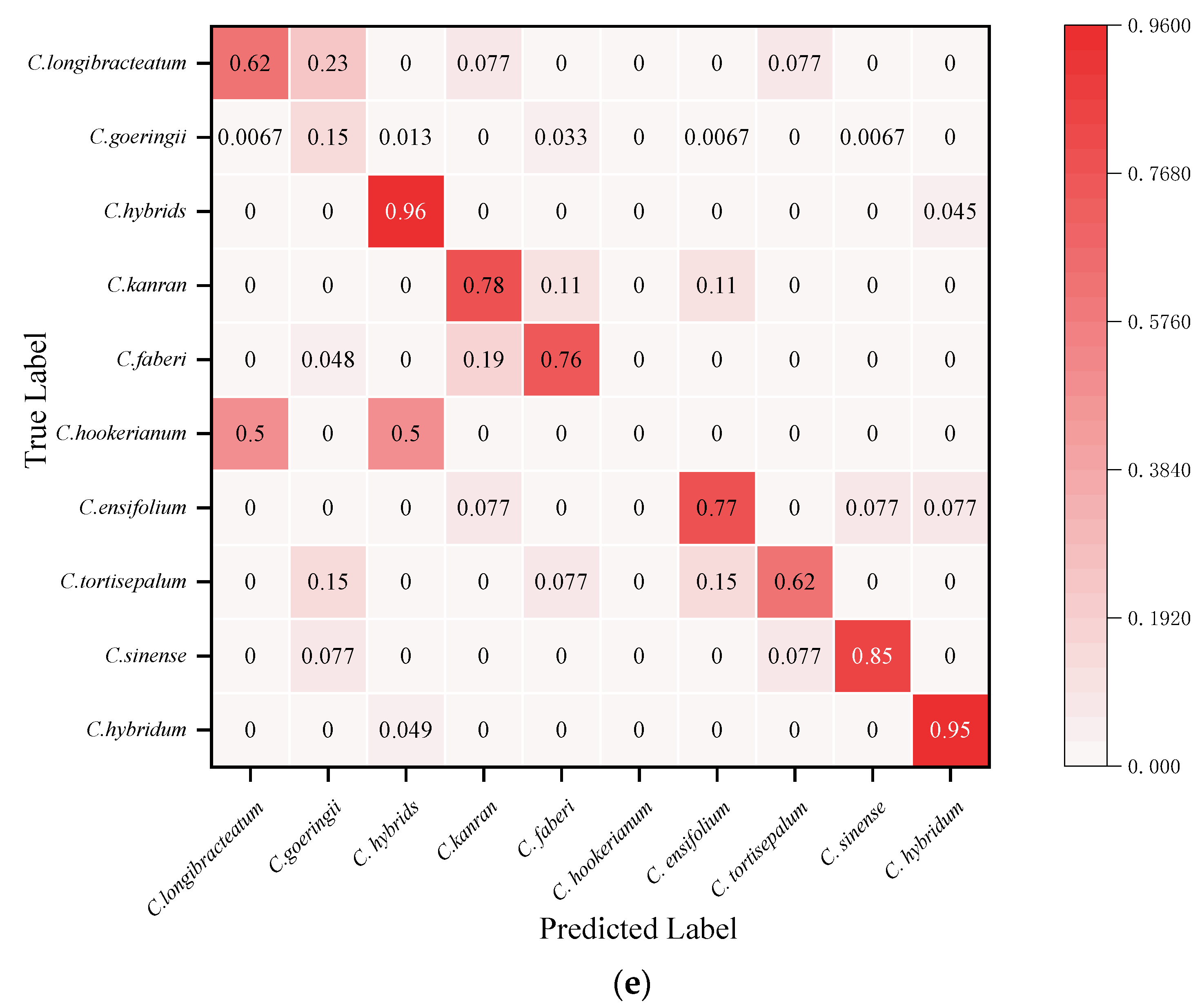
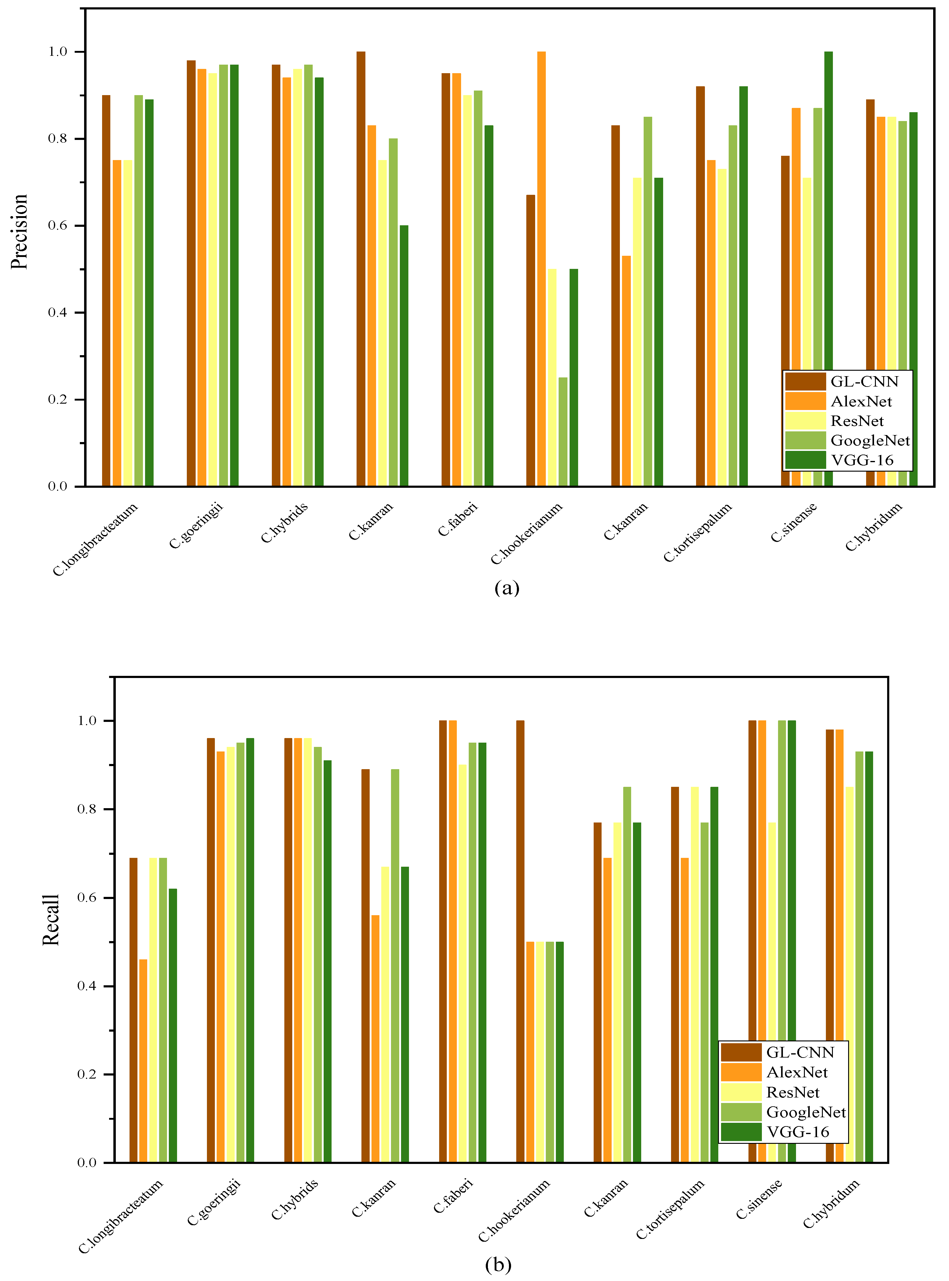
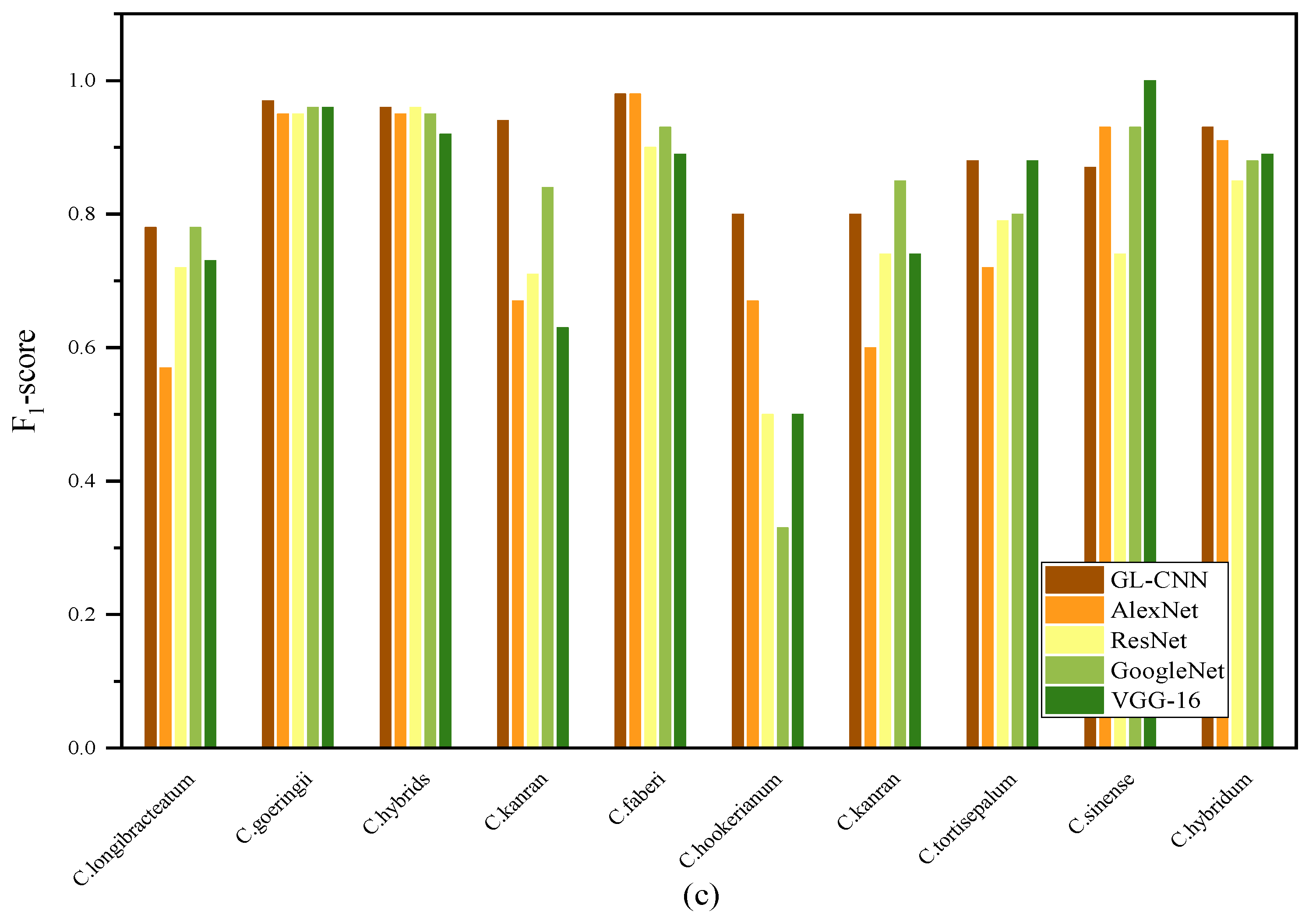
3.2. Model Performance Evaluation

The visual confusion matrix was used to count the classification results of different Cymbidium species (Figure 5). The true category (ordinates) and the predicted category (abscissa) were compared to obtain the classification rate of each species. The GL-CNN model has the highest prediction accuracy for C. faberi and C. hookerianum, with an accuracy rate of 100%, followed by C. hybridum, with an accuracy rate of 98% (Figure 5a). From the numerical distribution of the confusion matrix, it can be observed that all models have achieved high classification accuracy on C. hybrids, and their average classification rates have reached 95.6%. In addition, there have been more misclassifications between C. goeringii, C. longibracteatum, and C. tortisepalum. In general, the model GL-CNN built by this project has achieved a high individual classification rate in most orchid species recognition. The recognition performance of VGG16 is poor, and there is a serious misclassification phenomenon.
Figure 6 shows the precision, recall, and F1-score of 5 models for classifying 10 Cymbidium species. Among them, the precision, recall, and F1-score of each model on C. goeringii and C. hybrids all reached high values. On the contrary, the precision, recall, and F1-score of the five models on the C. hookerianum are quite different. GL-CNN has the highest precision, with an average of 89%. ResNet’s average precision is the lowest, only 78%, indicating that there are many samples misclassified under this method. Using the AlexNet model, many samples were misclassified to other varieties (the average recall rate was 0.78) because the differences between the samples were small, and there was a certain degree of difficulty in recognition. The precision and recall rate of different models are quite different, which indicates that the recognition difference of each model is more prominent in the categories that are more difficult to distinguish, showing a certain degree of unstable performance. In addition, GL-CNN showed high precision and recall rates in 10 different species of Cymbidium, indicating its strong ability to extract nuances.
Table 2 lists the average accuracy of the five models in order to further and comprehensively evaluate the effectiveness of the model. It can be observed from the table that GL-CNN has achieved the highest average accuracy of 94.13%. Compared with other models, GL-CNN has greatly improved the accuracy of classification. Correspondingly, VGG16 only achieves an average accuracy of 88.60%, which is significantly lower than GL-CNN.

4. Discussion

CNN is a method that combines an artificial neural network and deep learning with good fault tolerance and adaptability [42]. At the same time, it also has the advantages of automatic feature extraction, weight sharing, and a good combination of input image and network structure [27]. It is widely used in plant species identification, pest identification, weed identification, and other fields [43,44,45]. Existing CNN-based classification methods mainly focus on single-scale image data sets [27]. Therefore, there is an urgent need to design a fusion network that integrates the advantages of multiple features, which will greatly improve classification performance. This research proposed a two-scale CNN model, GL-CNN, which can extract features of different granularities from images of two scales, thereby enriching useful feature information, and ultimately improving the recognition ability of the model [26,27]. Researchers found that increasing the number of layers and units in the network will bring significant performance improvements, but it is prone to overfitting, explosion, or the disappearance of gradients [26]. To solve the above problems, a compact bilinear pooling method was proposed by Gao et al. [46], which can reduce the dimensionality while maintaining accuracy. Our experiment used a cascade fusion strategy to fit the two-scale features obtained from the two branches. Meanwhile, ReLU6, dropout, and other methods were used to alleviate potential overfitting problems. In the process of network training, dropout reduces the running time by randomly ignoring a certain proportion of hidden layer nodes, which can effectively reduce the interdependence between neurons, thereby extracting independent important features and inhibiting network overfitting.
In model training, the choice of feature extractor can affect the accuracy and speed of model detection. As the number of feature extractor layers increases, the network can extract higher-dimensional sample features, but the increase in network depth will affect the update signal of each layer and affect detection accuracy [47,48]. As classic feature extractors, AlexNet, ResNet, GoogleNet, and VGGNet are mostly used for image classification and recognition [48,49]. This study has shown that compared with the four typical models, GL-CNN has obvious accuracy and computational advantages, and the model accuracy is as high as 94%. An unexpected phenomenon is that the two excellent models (VGGNet and ResNet) did not achieve the desired performance, especially VGGNet, which obtained the lowest results, with a model accuracy of only 88.6%. The reason for this phenomenon is that the VGGNet training speed is very slow, and the weight of the network architecture itself is very large. In the case of many parameters and insufficient image data, the excellent classification effect cannot be exerted [49,50]. ResNet’s network connection is also very complicated and requires a lot of calculations. Therefore, they need a large data set to complete the convergence of the model [50]. In contrast, GoogLeNet, and AlexNet contain fewer parameters, a relatively simpler structure, and better training effects than VGGNet and ResNet [27]. As the best training model, GL-CNN has a slight advantage over GoogleNet in accuracy. The parameters and calculations of GL-CNN are significantly smaller, and it is easy to construct and apply. When the orchid image with more background information is adjusted to 224 × 224, a great deal of fine-grained information will be lost, which prevents the network from learning more in-depth and sufficient details. This situation can lead to poor network performance. GL-CNN can obtain global and local information and cascade the two parts together to extract detailed context features, which helps to expand the input features and improve classification accuracy.
Deep learning is still data-driven, and the size and quality of the data set will directly affect the effectiveness of network training [26]. Due to the limitation of the data set size, it may be difficult to train CNN. This study found that the precision, recall, and F1-score of each model on C. hookerianum are quite different. This is due to the small sample size of C. hookerianum, which makes the stability performance of the model different. Therefore, the training model is not sensitive enough to recognize the experimental samples. By increasing the number of such images, the compatibility of the classification model for different Cymbidium species can be improved.

5. Conclusions

In this study, a Cymbidium classification method based on the GL-CNN was proposed. It consists of two CNN networks with comparable weight, which helps expand the input features and improve classification accuracy. The cascade fusion strategy was used to fit the multiscale features obtained from the two branches. ReLU6 and dropout were used to prevent gradient explosion and alleviate the problem of overfitting. The end-to-end training was realized, and the robustness of the model was enhanced. Comparing GL-CNN with four classic models (AlexNet, ResNet50, GoogleNet, and VGG16), the results showed that GL-CNN achieved the highest classification prediction accuracy with a value of 94.13%.
In summary, the GL-CNN model used in this paper integrates multiscale information through the network, expands the number of features, has high detection accuracy, and can effectively identify different species of Cymbidium.

Author Contributions

Q.F. and C.L. conceived the ideas and designed the methodology; Q.F. collected and analyzed the data and wrote the manuscript; C.L. guided the data analysis and reviewed the manuscripts; F.Z., R.R., L.Q., X.Z. and C.L. supervised all stages of the experiment. All authors have read and agreed to the published version of the manuscript.

Funding

This research was supported by the Hangzhou Agriculture and Social Development Project (20201203B104).

Institutional Review Board Statement

Not applicable.

Informed Consent Statement

Not applicable.

Data Availability Statement

Data are contained within the article.

Conflicts of Interest

The authors declare no conflict of interest.

References

  1. Dressler, R.L. Phylogeny and Classification of the Orchid Family; Cambridge University Press: Cambridge, UK, 1993. [Google Scholar]
  2. Sharma, S.K.; Rajkumari, K.; Kumaria, S.; Tandon, P.; Rao, S.R. Karyo-morphological characterization of natural genetic variation in some threatened Cymbidium species of Northeast India. Caryologia 2010, 63, 99–105. [Google Scholar] [CrossRef] [Green Version]
  3. Lee, Y.-M.; Kim, M.-S.; Lee, S.-I.; Kim, J.-B. Review on breeding, tissue culture and genetic transformation systems in Cymbidium. J. Plant Biotechnol. 2010, 37, 357–369. [Google Scholar] [CrossRef] [Green Version]
  4. Wang, H.-Z.; Lu, J.-J.; Hu, X.; Liu, J.-J. Genetic variation and cultivar identification in Cymbidium ensifolium. Plant Syst. Evol. 2011, 293, 101–110. [Google Scholar] [CrossRef]
  5. Ning, H.; Ao, S.; Fan, Y.; Fu, J.; Xu, C. Correlation analysis between the karyotypes and phenotypic traits of Chinese cymbidium cultivars. Hortic. Environ. Biotechnol. 2018, 59, 93–103. [Google Scholar] [CrossRef]
  6. Guo, F.; Niu, L.-X.; Zhang, Y.-L. Phenotypic Variation of Natural Populations of Cymbidium faberi in Zhashui. North Hortic. 2010, 18, 91–93. [Google Scholar]
  7. Sharma, S.K.; Kumaria, S.; Tandon, P.; Rao, S.R. Assessment of genetic variation and identification of species-specific ISSR markers in five species of Cymbidium (Orchidaceae). J. Plant Biochem. Biotechnol. 2013, 22, 250–255. [Google Scholar] [CrossRef]
  8. Lu, J.; Hu, X.; Liu, J.; Wang, H. Genetic diversity and population structure of 151 Cymbidium sinense cultivars. J. Hortic. For. 2011, 3, 104–114. [Google Scholar]
  9. Lee, D.-G.; Koh, J.-C.; Chung, K.-W. Determination and application of combined genotype of simple sequence repeats (SSR) DNA marker for cultivars of Cymbidium goeringii. Hortic. Sci. Technol. 2012, 30, 278–285. [Google Scholar] [CrossRef]
  10. Obara-Okeyo, P.; Kako, S. Genetic diversity and identification of Cymbidium cultivars as measured by random amplified polymorphic DNA (RAPD) markers. Euphytica 1998, 99, 95–101. [Google Scholar] [CrossRef]
  11. LeCun, Y.; Bengio, Y.; Hinton, G. Deep learning. Nature 2015, 521, 436–444. [Google Scholar] [CrossRef]
  12. Tian, C.; Xu, Y.; Fei, L.; Yan, K. Deep learning for image denoising: A survey. In Proceedings of the International Conference on Genetic and Evolutionary Computing, Springer, Singapore, 14–17 December 2018; pp. 563–572. [Google Scholar]
  13. Albawi, S.; Mohammed, T.A.; Al-Zawi, S. Understanding of a convolutional neural network. In Proceedings of the 2017 International Conference on Engineering and Technology (ICET), Antalya, Turkey, 21–23 August 2017; pp. 1–6. [Google Scholar]
  14. Cengil, E.; Çinar, A.; Güler, Z. A GPU-based convolutional neural network approach for image classification. In Proceedings of the 2017 International Artificial Intelligence and Data Processing Symposium (IDAP), Malatya, Turkey, 16–17 September 2017; pp. 1–6. [Google Scholar]
  15. Dyrmann, M.; Karstoft, H.; Midtiby, H.S. Plant species classification using deep convolutional neural network. Biosys. Eng. 2016, 151, 72–80. [Google Scholar] [CrossRef]
  16. Yalcin, H.; Razavi, S. Plant classification using convolutional neural networks. In Proceedings of the 2016 Fifth International Conference on Agro-Geoinformatics (Agro-Geoinformatics), Tianjin, China, 18–20 July 2016; pp. 1–5. [Google Scholar]
  17. Ma, J.; Du, K.; Zheng, F.; Zhang, L.; Gong, Z.; Sun, Z. A recognition method for cucumber diseases using leaf symptom images based on deep convolutional neural network. Comput. Electron. Agric. 2018, 154, 18–24. [Google Scholar] [CrossRef]
  18. Patel, I.; Patel, S. An Optimized Deep Learning Model for Flower Classification Using NAS-FPN and Faster R-CNN. Int. J. Sci. Technol. Res. 2020, 9, 5308–5318. [Google Scholar]
  19. Liu, Y.H. Feature extraction and image recognition with convolutional neural networks. J. Phys. Conf. Ser. 2018, 1087, 062032. [Google Scholar] [CrossRef]
  20. Workman, S.; Jacobs, N. On the location dependence of convolutional neural network features. In Proceedings of the IEEE Conference on Computer Vision and Pattern Recognition Workshops, Boston, MA, USA, 7–12 June 2015; pp. 70–78. [Google Scholar]
  21. Li, W.; Wu, G.; Zhang, F.; Du, Q. Hyperspectral image classification using deep pixel-pair features. IEEE Trans. Geosci. Remote Sens. 2016, 55, 844–853. [Google Scholar] [CrossRef]
  22. Hiary, H.; Saadeh, H.; Saadeh, M.; Yaqub, M. Flower classification using deep convolutional neural networks. IET Comput. Vis. 2018, 12, 855–862. [Google Scholar] [CrossRef]
  23. Dias, P.A.; Tabb, A.; Medeiros, H. Apple flower detection using deep convolutional networks. Comput. Ind. 2018, 99, 17–28. [Google Scholar] [CrossRef] [Green Version]
  24. Alaslani, M.G. Convolutional neural network based feature extraction for iris recognition. Int. J. Comput. Sci. Inf. Technol. (IJCSIT) 2018, 10, 65–78. [Google Scholar] [CrossRef] [Green Version]
  25. Huang, K.; Liu, X.; Fu, S.; Guo, D.; Xu, M. A lightweight privacy-preserving CNN feature extraction framework for mobile sensing. IEEE Trans. Dependable Secur. Comput. 2019, 18, 1441–1455. [Google Scholar] [CrossRef]
  26. Xie, G.-S.; Zhang, X.-Y.; Yang, W.; Xu, M.; Yan, S.; Liu, C.-L. LG-CNN: From local parts to global discrimination for fine-grained recognition. Pattern Recognit. 2017, 71, 118–131. [Google Scholar] [CrossRef]
  27. Hao, X.; Jia, J.; Khattak, A.M.; Zhang, L.; Guo, X.; Gao, W.; Wang, M. Growing period classification of Gynura bicolor DC using GL-CNN. Comput. Electron. Agric. 2020, 174, 105497. [Google Scholar] [CrossRef]
  28. Simonyan, K.; Zisserman, A. Very deep convolutional networks for large-scale image recognition. arXiv 2014, arXiv:1409.1556. [Google Scholar]
  29. Chao, X.; Sun, G.; Zhao, H.; Li, M.; He, D. Identification of apple tree leaf diseases based on deep learning models. Symmetry 2020, 12, 1065. [Google Scholar] [CrossRef]
  30. Neupane, B.; Horanont, T.; Aryal, J. Deep Learning-Based Semantic Segmentation of Urban Features in Satellite Images: A Review and Meta-Analysis. Remote Sens. 2021, 13, 808. [Google Scholar] [CrossRef]
  31. Zhou, Q.; Situ, Z.; Teng, S.; Chen, G. Convolutional Neural Networks—Based Model for Automated Sewer Defects Detection and Classification. J. Water Resour. Plan. Manag. 2021, 147, 04021036. [Google Scholar] [CrossRef]
  32. Huang, K.; Li, C.; Zhang, J.; Wang, B. Cascade and Fusion: A Deep Learning Approach for Camouflaged Object Sensing. Sensors 2021, 21, 5455. [Google Scholar] [CrossRef]
  33. Lin, G.; Shen, W. Research on convolutional neural network based on improved Relu piecewise activation function. Procedia Comput. Sci. 2018, 131, 977–984. [Google Scholar] [CrossRef]
  34. Agarap, A.F. Deep learning using rectified linear units (relu). arXiv 2018, arXiv:1803.08375. [Google Scholar]
  35. Srivastava, N.; Hinton, G.; Krizhevsky, A.; Sutskever, I.; Salakhutdinov, R. Dropout: A simple way to prevent neural networks from overfitting. J. Mach. Learn. Res. 2014, 15, 1929–1958. [Google Scholar]
  36. Hu, K.; Zhang, Z.; Niu, X.; Zhang, Y.; Cao, C.; Xiao, F.; Gao, X. Retinal vessel segmentation of color fundus images using multiscale convolutional neural network with an improved cross-entropy loss function. Neurocomputing 2018, 309, 179–191. [Google Scholar] [CrossRef]
  37. Dozat, T. Incorporating nesterov momentum into adam. In Proceedings of the 4th International Conference on Learning Representations, Workshop Track, Caribe Hilton, San Juan, Puerto Rico, 2–4 May 2016. [Google Scholar]
  38. Yu, W.; Yang, K.; Bai, Y.; Xiao, T.; Yao, H.; Rui, Y. Visualizing and comparing AlexNet and VGG using deconvolutional layers. In Proceedings of the 33rd International Conference on International Conference on Machine Learning, New York, NY, USA, 19–24 June 2016. [Google Scholar]
  39. Ballester, P.; Araujo, R.M. On the performance of GoogLeNet and AlexNet applied to sketches. In Proceedings of the Thirtieth AAAI Conference on Artificial Intelligence, Phoenix, AZ, USA, 12–17 February 2016. [Google Scholar]
  40. Gao, M.; Chen, J.; Mu, H.; Qi, D. A Transfer Residual Neural Network Based on ResNet-34 for Detection of Wood Knot Defects. Forests 2021, 12, 212. [Google Scholar] [CrossRef]
  41. Yacouby, R.; Axman, D. Probabilistic Extension of Precision, Recall, and F1 Score for More Thorough Evaluation of Classification Models. In Proceedings of the First Workshop on Evaluation and Comparison of NLP Systems; Association for Computational Linguistics: Stroudsburg, PA, USA, 2020; Volume 202, pp. 79–91. [Google Scholar]
  42. Azman, A.A.; Ismail, F.S. Convolutional Neural Network for Optimal Pineapple Harvesting. ELEKTRIKA-J. Electr. Eng. 2017, 16, 1–4. [Google Scholar]
  43. Saleem, G.; Akhtar, M.; Ahmed, N.; Qureshi, W.S. Automated analysis of visual leaf shape features for plant classification. Comput. Electron. Agric. 2019, 157, 270–280. [Google Scholar] [CrossRef]
  44. Liu, J.; Pi, J.; Xia, L. A novel and high precision tomato maturity recognition algorithm based on multi-level deep residual network. Multimed. Tools Appl. 2020, 79, 9403–9417. [Google Scholar] [CrossRef]
  45. Esgario, J.G.M.; Krohling, R.A.; Ventura, J.A. Deep learning for classification and severity estimation of coffee leaf biotic stress. Comput. Electron. Agric. 2020, 169, 105162. [Google Scholar] [CrossRef] [Green Version]
  46. Gao, Y.; Beijbom, O.; Zhang, N.; Darrell, T. Compact bilinear pooling. In Proceedings of the 2016 IEEE Conference on Computer Vision and Pattern Recognition (CVPR), Las Vegas, NV, USA, 27–30 June 2016; pp. 317–326. [Google Scholar]
  47. Yuan, Z.-W.; Zhang, J. Feature extraction and image retrieval based on AlexNet. In Proceedings of the Eighth International Conference on Digital Image Processing (ICDIP 2016), Chengdu, China, 20–22 May 2016; p. 100330E. [Google Scholar]
  48. Thenmozhi, K.; Reddy, U.S. Crop pest classification based on deep convolutional neural network and transfer learning. Comput. Electron. Agric. 2019, 164, 104906. [Google Scholar] [CrossRef]
  49. Sethy, P.K.; Barpanda, N.K.; Rath, A.K.; Behera, S.K. Nitrogen deficiency prediction of rice crop based on convolutional neural network. J. Ambient. Intell. Humaniz. Comput. 2020, 11, 5703–5711. [Google Scholar] [CrossRef]
  50. Yaqoob, M.K.; Ali, S.F.; Bilal, M.; Hanif, M.S.; Al-Saggaf, U.M. ResNet Based Deep Features and Random Forest Classifier for Diabetic Retinopathy Detection. Sensors 2021, 21, 3883. [Google Scholar] [CrossRef]
Figure 1. Examples of pictures of 10 Cymbidium species.
Horticulturae 08 00470 g001
Figure 2. Schematic diagram of two-scale image acquisition.
Horticulturae 08 00470 g002
Figure 3. Examples of the effects before and after image enhancement.
Horticulturae 08 00470 g003
Figure 4. GL-CNN network structure diagram.
Horticulturae 08 00470 g004
Figure 5. Test set confusion matrix: (a) GL-CNN; (b) AlexNet; (c) ResNet; (d) GoogleNet; (e) VGGNet.
Horticulturae 08 00470 g005aHorticulturae 08 00470 g005bHorticulturae 08 00470 g005c
Figure 6. Precision (a), recall (b), and F1-score (c) of each model on different Cymbidium species.
Horticulturae 08 00470 g006aHorticulturae 08 00470 g006b
Table 1. Details of GL-CNN hidden layer parameters.
LayerTypeSizeNumber of CoresStep SizeOutput SizeNumber of ConvolutionsNumber of Neurons
Input----224 × 224 × 3--
Conv11Convolution11 × 1196454 × 54 × 96(11 × 11 + 1) × 9654 × 54 × 96
Pool11Mean-pooling3 × 3-226 × 26 × 96-26 × 26 × 96
Conv12Convolution5 × 596126 × 26 × 256(5 × 5 + 1) × 9626 × 26 × 96
Pool12Mean-pooling3 × 3-212 × 12 × 96-12 × 12 × 96
Conv13Convolution3 × 3192112 × 12 × 384(3 × 3 + 1) × 19212 × 12 × 192
Conv14Convolution3 × 3256112 × 12 × 384(3 × 3 + 1) × 25612 × 12 × 256
Pool13Mean-pooling3 × 3-25 × 5 × 256-5 × 5 × 256
FC11Fully connected1 × 14096-1 × 1 × 4096(1 × 1 + 1) × 40961 × 1 × 2048
Conv21Convolution5 × 596375 × 75 × 96(5 × 5 + 1) × 9675 × 75 × 96
Pool21Mean-pooling3 × 3-325 × 25 × 96-25 × 25 × 96
Conv22Convolution5 × 596125 × 25 × 256(5 × 5 + 1) × 9625 × 25 × 96
Pool22Mean-pooling3 × 3-212 × 12 × 96-12 × 12 × 96
Conv23Convolution3 × 3192112 × 12 × 384(3 × 3 + 1) × 19212 × 12 × 192
Conv24Convolution3 × 3256112 × 12 × 384(3 × 3 + 1) × 25612 × 12 × 256
Conv25Convolution3 × 3256112 × 12 × 384(3 × 3 + 1) × 25612 × 12 × 256
Pool23Mean-pooling3 × 3-25 × 5 × 256-5 × 5 × 256
FC21Fully connected1 × 14096-1 × 1 × 4096(1 × 1 + 1) × 40961 × 1 × 2048
CasCascade---1 × 1 × 8192-1 × 1 × 8192
FC2Fully connected1 × 14096-1 × 1 × 4096(1 × 1 + 1) × 40961 × 1 × 4096
FC3Fully connected1 × 11000-1 × 1 × 1000(1 × 1 + 1) × 10001 × 1 × 1000
OutputOutput1 × 110-1 × 1 × 10--
Table 2. Average accuracy of each model.
GL-CNNAlexNetResNetGoogleNetVGGNet
Average accuracy (%)94.1390.0689.4792.1588.60
Publisher’s Note: MDPI stays neutral with regard to jurisdictional claims in published maps and institutional affiliations.

