Article

VIS-NIR Modeling of Hydrangenol and Phyllodulcin Contents in Tea-Hortensia (Hydrangea macrophylla subsp. serrata)

1
Renewable Resources, Institute of Crop Science and Resource Conversation, University of Bonn, Klein-Altendorf 2, 53359 Rheinbach, Germany
2
Symrise AG, Mühlenfeldstr. 1, 37603 Holzminden, Germany
3
Horticultural Sciences, Institute of Crop Science and Resource Conversation, University of Bonn, Auf dem Hügel 6, 53121 Bonn, Germany
4
Field Lab, Campus Klein-Altendorf, University of Bonn, Klein-Altendorf 2, 53359 Rheinbach, Germany
*
Author to whom correspondence should be addressed.
These authors contributed equally to this work.
Horticulturae 2022, 8(3), 264; https://doi.org/10.3390/horticulturae8030264
Submission received: 9 February 2022 / Revised: 16 March 2022 / Accepted: 16 March 2022 / Published: 18 March 2022

Abstract

:
Hyperspectral data are commonly used for the fast and inexpensive quantification of plant constituent estimation and quality control as well as in research and development applications. Based on chemical analysis, different models for dihydroisocoumarins (DHCs), namely hydrangenol (HG) and phyllodulcin (PD), were built using a partial least squares regression (PLSR). While HG is common in Hydrangea macrophylla, PD only occurs in cultivars of Hydrangea macrophylla subsp. serrata, also known as ‘tea-hortensia’. PD content varies significantly over the course of the growing period. For maximizing yield, a targeted estimation of PD content is needed. Nowadays, DHC contents are determined via UPLC, a time-consuming and a destructive method. In this research article we investigated PLSR-based models for HG and PD using three different spectrometers. Two separate trials were conducted to test for model quality. Measurement conditions, namely fresh or dried leaves and black or white background, did not influence model quality. While highly accurate modeling of HG and PD for single plants was not possible, the determination of the mean content on a larger scale was successful. The results of this study show that hyperspectral modeling as a decision support for farmers is feasible and provides accurate results on a field scale.

1. Introduction

Hydrangea macrophylla subsp. serrata has shown to be of interest for its content of the dihydroisocoumarin (DHC) glycosides hydrangenol (HG) and phyllodulcin (PD). Synthesis of DHCs in H. macrophylla subsp. serrata are driven by the shikimic pathway and coumaric acid. Intermediates during synthesis are stilbenecarboxylates in the mevalonate pathway that are enabled by a specific polyketide synthase [1]. During synthesis of PD, HG functions as a precursor [2]. HG and PD contents are influenced by seasonal changes and leaf age, and seem to be predetermined by genetics more than environment [3,4]. The popular name for H. macrophylla subsp. serrata, ‘tea-hortensia’—as proposed by Moll et al. [4], is based on the plant’s original use as a ceremonial tea called Amacha (Japanese for 甘い = amai = sweet, 茶 = cha = tea) [5]. The characteristic taste is caused by PD [6]. Furthermore, HG and PD provide multiple positive benefits. Among these provided benefits, HG enhances the growth-promoting activity from gibberellin [7]. Analogous to PD, HG shows anti-fungal effects [8], but also affects the activation of hyaluronidase and possesses anti-allergenic activities [9]. In BV-2 microglial cells, HG inhibits lipopolysaccharide-induced nitric oxide production [10]. Inhibition of the proliferation, migration, and invasion of EJ bladder cancer was investigated in HG [11], as well as for UV-induced skin damage reduction in mice [12]. Leaf extracts from Hydrangea macrophylla L. were shown to have plant growth promoting effects in mungbean (Vigna radiata L.) which may be due to hormonal effects as well as the micro- and macronutrients in the extracts [13]. The beneficial properties of PD include anti-fungal [14], anti-ulcer, anti-allergic [15], anti-bacterial [16] and anti-inflammatory properties [17]. In vitro, and on a microsomal level, PD is a potent inhibitor of lipid peroxidation [15]. Additionally, further animal experiments investigated the enhancement of cyclic AMP-induced steroidogenesis in bovine adrenocortical cells [18]. Other animal experiments also found that obesity-related symptoms in mice could be reduced [19,20]. The positive effects of PD as a malaria treatment [21], as well as increasing cellular viability and as a protective measure against oxygenation-induced injuries in PC12 cells [22] have also been investigated.
Until now, the quantification of HG and PD has been performed using ultra performance liquid chromatography (UPLC), with one possible protocol introduced by Moll et al. (2021) [4]. While providing advantages in comparison to conventional HPLC, the analysis can be time consuming, depending on the specific compounds [23], even if UPLC has been shown to be up to nine times faster than HPLC [24]. Despite being advantageous in comparison to other techniques [25], UPLC is not suitable to be performed by farmers for real-time estimations in field for PD content quantifications or prediction.
Hyperspectral modeling of the VIS-NIR and NIR regions have been shown to be able to model leaf constituents in natural products [26] over a wide range of plants (coffee, tea, cocoa, tobacco), spices, medicinal and aromatic plants in general [27] and to model the shelf life of products [28]. Additionally, the discrimination of plants using a NIRS-based chemometric evaluation is a promising field of research [29]. On a leaf-based level, contents of flavonoids [30] or terpenoids [31] were investigated using infrared spectroscopy and chemometrics. NIR modeling is used for modeling volatile organic compounds (VOC) in Mentha [32]. Besides constituent analysis and estimation, the yield presents a field of research as well, for instance in alfalfa (Medicago sativa L.) [33] or wheat (Triticum aestivum) [34]. For rice yield, the possibilities of using multispectral data from drones was investigated as well [35].
In the system of hyperspectral measurements, three factors influence the data acquisition: the scene (the observable space in front of the spectrometer), the sensor system, and the processing system [36]. Portable devices allow for satisfying results from VIS-NIR spectra as well [28].
We hypothesized that measurement conditions do not influence model accuracy and that it is possible to use VIS-NIR spectrometers to model for both the HG and PD contents. Based on these results, the suitability of models based on the handheld PolyPen RP400 was to be investigated as a simple and fast proxy for HG and PD contents on a field scale. This would enable farmers to find optimized harvest dates during the season and act as a decision support in tea-hortensia cultivation.
This article provides the first assessment of hyperspectral modeling as a decision support for farmers as well as for scientific purposes in the field of tea-hortensia and the dihydroisocoumarins HG and PD. Seasonal changes [3] lead to uncertainties of ideal harvest time, as peaks in PD accumulation might differ between cultivars. Therefore, a fast quantification of HG and PD is needed on a field scale. Additionally, this study further investigates the possibilities of cultivar differentiation as well as the impact of measurement conditions on model quality.

2. Materials and Methods

2.1. Spectrometer Set-Up

Multiple setups of spectrometers were used for the experiments presented in this study. First, in 2019, two spectrometers from Ocean Insight (Orlando, FL, USA) were used, namely the ‘Red Tide USB650 Fiber Optic Spectrometer’ (350–1000 nm), from now on shortened to ‘Red Tide’, and the ‘Flame-NIR Miniature Spectrometer’ (950–1650 nm), in this study shortened to ‘Flame-NIR’. The Red Tide provides a resolution of 651 pixels per spectrum (2 nm full-width at half-maximum (FWHM)), equal to one datapoint per nm with a signal-to-noise ratio of 250:1. The Flame-NIR signal-to-noise ratio is 6000:1 providing 128 datapoints for its spectrum with a resolution of 10 nm FWHM. Both spectrometers were connected to an external Ocean Insight Tungsten Halogen Light Source HL-2000-HP using a QR200-12-MIXED fiber optic. The ‘SMA connector’ was inserted at maximum and the ‘attenuator’ was pulled out at the maximum. The probe was fixated 1 mm above the sample at an angle of 90° to the leaf surfaces (specular reflectance) using an RPH-1 reflection probe holder. Spectra were collected in reflectance mode and calibration was performed using the Spectroscopy Application Wizard built into the OceanView 1.6.7 software and using a WS1-Diffuse Reflectance Standard. In the first experiment, the spectrometers were used separately to measure four spots per leaf. The integration time was set to 50 ms and 733 ms for the Red Tide and Flame-NIR, respectively. Additionally, both spectrometers were used with 2 scans to average and a boxcar width of 5. Spectra of the four scanning spots were then averaged for further calculations.
In the second experiment, in 2021, the spectrometers were used simultaneously to measure the same spot on a sample. Integration time was set to 6 ms for Red Tide with 25 scans to average and 320 ms for Flame-NIR with 5 scans to average. Again, a boxcar width of 5 was used. Recalibration was done after about 20 to 30 measurements using a white reference and a dark spectrum. Data collection and processing were performed using OceanView 1.6.7 and Microsoft Excel 2019.
Besides stationary spectrometers, the handheld PolyPen RP400 (UV-VIS), from now on referred to as ‘PolyPen’, by Photon Systems Instruments (Brno, Czech Republic), covering a detection range from 380–780 nm with 256 datapoints and a resolution of 8 nm half-width at half-maximum was used to investigate reflectance spectra. Data collection and processing for the PolyPen were performed via SpectraPen 1.0.0.5 and Microsoft Excel 2019.
The original spectrometer data for the experiments are shown in Supplementary Materials Table S1 (2019, Ocean Insight), Table S2 (2021, Ocean Insight), and Table S3 (2021, PolyPen).

2.2. Plant Material and Cultivation

Plant material was obtained from commercial breeders for both experiments. For the first experiment, Kühne Jungpflanzen, Claus Kühne (Dresden, Germany) delivered the plants, and for the second experiment, Kötterheinrich Hortensienkulturen e.K. (Lengerich, Germany). Plant material for the first measurements was delivered to the Institute of Crop Science and Resource Conservation—Renewable Resources in May 2019 as rooted cuttings in 6 × 8 multipot trays and potted in Jiffy-Pots #130 (Jiffy Products International BV, Zwijndrecht, Netherlands) in June 2019 into ‘Einheitserde ED73’ (Einheitserdewerke Werkverband e.V., Sinntal-Altgronau, Germany). Until measurement, all plants were cultivated under the same conditions in a greenhouse and irrigated daily. A total of 5000 plants per tea-hortensia cultivars ‘Amagi Amacha’, ‘Oamacha’ and ‘Odoriko Amacha’ were cultivated in this regime. In May 2019, plants from the same production cycle were delivered to Symrise AG (Holzminden, Germany) as well. Those plants from tea-hortensia cultivar ‘Oamacha’ were planted as part of a small exhibition garden.

2.3. Experimental Design

The study comprised of two separate measurement dates. The first measurement was part of an experiment carried out on 9 July 2019 to gain an understanding of measurement specifics. Therefore, the three tea-hortensia cultivars (‘Amagi Amacha’, ’Oamacha’, ‘Odoriko Amacha’) were analyzed using a black and a white background plate separately. Additionally, fresh leaves were measured after harvest and after drying at 40 °C for 72 h. Sample selection was performed by randomly taking 20 plants from a plant stock consisting of 5000 plants per cultivar and measuring both upper fully developed leaves for each background and leaf water status.
Based on the first results, a second trial was performed. The second block of measurements were part of an experiment carried out on 20 August in 2021 using in-field cultivated H. macrophylla subsp. serrata ‘Oamacha’, again using Red Tide and Flame-NIR. In this trial, a total of 304 single fully developed upper leaves were taken to be measured as fresh leaves on a black background. To avoid wilting, 30 to 40 samples were collected immediately before data acquisition, so that the time slot between harvest and measurement was no longer than 30 min. Sample selection was again carried out by randomly taking leaves from in-plants. The reflectance spectra from 61 of these leaves were additionally taken using the PolyPen, where the mean value of four measurements was calculated.

2.4. Analysis of Hydrangenol and Phyllodulcin

The analysis of hydrangenol and phyllodulcin was performed at Symrise AG (Holzminden, Germany) on a Waters Acquity UPLC® I-Class. An Acquity UPLC ελ PDA detector combined with a commercially available reversed phase C18 column (Luna Omega 1.6 µm Polar C18 50 × 2.1 mm) was used. The procedure was performed according to the protocol for hydrangenol and phyllodulcin quantification for tea-hortensias (Moll et al., 2021) [4].

2.5. Outlier Detection and Spectra Pre-Processing

Errors in a dataset, disturbing effects like spectral noise and many other factors influence data analysis and can affect model quality, thus data pre-processing has proven to be advisable [37]. First, DHC contents (HG and PD) were checked for outliers. Samples with values exceeding three times the interquartile range of the 0.25 tail quantile were excluded from further calculations. Furthermore, the raw spectra were graphically examined and samples with curves strongly shifted on the x-axis were manually removed. In addition, a penalized basis spline (P-spline) model, which minimizes residuals and avoids overfitting at the same time [38,39], was fitted to the reflectance measurements to detect multivariate outliers within the score plot of the first and second principal components. To get an overview, models were developed using leave-one-out cross validation. The model is developed with n-1 training data (n corresponds to the number of samples) and the holdout sample is used for calibration. This process is repeated n times [40]. After cross validation, another sample was discarded due to a high Hotellings T2-statistic (α = 0.05). This method is suitable for correlated variables and is considered as an enhancement of the Student’s t-distribution for multivariate data sets [41]. The procedures resulted in 40 spectra for ‘Oamacha’ and ‘Odoriko Amacha’ and 35 for ‘Amagi Amacha’ in 2019, as well as 296 spectra from the Ocean Insight spectrometers and 60 spectra for modeling with the PolyPen data in 2021.
Standard normal variate (SNV) transformation and Savitzky–Golay (SG) filters. including smoothing, or first- and second order derivatives, were the pre-processing methods in this study. SNV transformation corrects slope variations and scatter effects by first centering the individual spectra and then dividing them by their standard deviation [42]. Smoothing methods are suitable for reducing spectral noise [43]. Based on the moving average method, polynomial smoothing, also known as Savitzky–Golay (SG) smoothing, fits a polynomial function to the data of a chosen smoothing interval so that data are entered with different weights in the calculation of the value to be smoothed. This preserves the structure and spectral information, even with larger smoothing intervals [44]. In addition, the aligned SG polynomial functions fitted to the smoothing intervals can be derived [45]. The obtained derivatives of the spectra remove baseline shifts [46]. The optimal preprocessing methods have to be adapted individually for each model [47]. Here it was found that SNV transformation before SG processing showed the best results. Due to strong noise (observed via graphical inspection) of the SNV transformed spectra of the Red Tide spectrometer in 2021, the wavelength range below 400 nm was excluded from calculations. Afterwards, SG algorithms with 2nd to 8th degree polynomials with window points ranging from 11 to 61 were tested. A summary of the methods and wavelength ranges used for modeling can be found in Table 1. Pretreatments were conducted in JMP Pro 16.

2.6. Model Development

Models were implemented in JMP Pro 16 (SAS) by partial least squares regression (PLSR). PLSR has proven to be a practical and widely used tool for investigating spectroscopic data [48,49,50]. In contrast to multiple linear regression (MLR), this method enables processing of a large number of X-variables (here the wavelengths, also ‘predictors’ or X), which can be intercorrelated and occaisionally show strong noise [51]. The aim is to establish a relationship between the predictors and at least one Y-variable (here the HG or PD content, also ‘response’ or y), which allows for predictions of the latter [52]. Performing a principal component analysis of both the predictors and responses and intercorrelating them reduces the number of variables to a few PLS principal components (also called ‘factors’ or ‘latent variables’), which simplifies modeling and separates relevant information [53]. In order to determine the appropriate number of factors and prevent overfitting or underfitting, validation of the model is required [40]. Therefore, the samples were randomly split into three subsets: training, validation, and testing, that will later result in calibration, validation, and prediction models. The training set (composed of 70% of the samples) was used to estimate the calibration model parameters, the validation set (20%) was used within the algorithm to optimize the calibration model, whose ability to predict was assessed with the separate test set (10%) not involved in the model building process. For calibration model development, data were scaled to unit variances (standard deviation of 1 by dividing the data by their variables’ standard deviation) and centered to a mean value of zero (by subtracting variables average values from the data) [51]. Subsequently, all variables had the same impact on modeling in terms of variation and interpretation was simplified. NIPALS (non-linear iterative partial least squares) was chosen as the algorithm. As Hu et al. [54] reported, model performance can be affected by variable selection. So-called variable influence on projection (VIP) [55] values describe the importance of a variable (x) in explaining both X and y [51]. According to Wold et al., variables below a threshold of 1.0 can be removed. Models in this study were pruned until all variables were weighted with a factor greater than 0.8 [55].

2.7. Statistical Analysis

Parameters based on the determination of residuals (ei) can be used to assess the goodness of fit. Residuals are defined as the difference between the actual measured (yi) and predicted (ŷi) analyte concentrations and represent the remaining variance in the data that cannot be explained by the principal components [51]. In this study, both root mean square error (RMSE) as well as the coefficient of determination (R2) were specified for the different subsets: the training set, which correspond to the calibration model (Rc2 and RMSEC); the validation set (Rv2 and RMSEV); the test set, which correspond to the prediction set in common terminology (Rp2 and RMSEP) and the overall model (Rtotal2 and RMSEtotal). Equations are given in (1) and (2). Models with a low RMSE/root mean PRESS and a high R2 score were considered to be good.
RMSE = i = 1 n ( y i ŷ i ) 2 n
R 2 = 1 i = 1 n ( y i ŷ i ) 2 i = 1 n ( y i ȳ ) 2
  • n = number of samples (spectra), yi = measured reference value of the sample i,
  • ŷ = predicted value of the sample i, ȳ = mean value of all samples.
Statistical analysis of HG and PD contents in the three cultivars and comparison of models’ R2 regarding the spectrometers used and the partition of the sample sets was performed via analysis of variance (ANOVA) with the Tukey-HSD test as a post hoc procedure to determine homogenous subgroups at a p-value of p ≤ 0.05. Differences between ‘Oamacha’ datasets for Red Tide + Flame-NIR and PolyPen were investigated via a t-test (p ≤ 0.05) with significant differences marked with an asterisk (*).
For the detection of cultivars via hyperspectral models and the impact of measurement background, a discriminant analysis was performed using the cultivars, leaf water status, or backgrounds as the category and HG, PD, and both simultaneously from UPLC analysis as well as prediction models as the covariables.

3. Results

3.1. Hydrangenol and Phyllodulcin Contents

The analysis of hydrangenol and phyllodulcin revealed significant differences between the cultivars in 2019. The HG contents were highest in ‘Odoriko Amacha’ (4.787% ± 1.066%), followed by ‘Oamacha’ (1.514% ± 0.649%), and then ‘Amagi Amacha’ (0.293% ± 0.142%). Phyllodulcin did not show significant differences between ‘Oamacha’ (3.642% ± 0.692%) and ‘Amagi Amacha’ (3.906% ± 0.480%). Both cultivars yielded higher contents of PD than cultivar ‘Odoriko Amacha’ (1.794% ± 0.323%). In 2021, only ‘Oamacha’ was investigated. For both spectrometer setups used (Red Tide + Flame-NIR and PolyPen), different samples were taken out of the modeling process as described in the Material and Methods section regarding data pre-treatment and data elimination. Therefore, different means for HG and PD contents were calculated. For trial I (Red Tide + Flame-NIR) a mean HG content of 0.515% ± 0.133% and a mean PD content of 4.409% ± 0.264% were recorded. The analysis for trial II (PolyPen) revealed 0.545% ± 0.145% HG and 4.448% ± 0.270% PD. The statistical analysis determined no significant differences in mean constituent contents for HG and PD in ‘Oamacha’ that could be a result of different samples taken out of the calculations. The distribution of HG and PD contents by harvest year, trial, and cultivar is illustrated in Figure 1.

3.2. Differentiation of Cultivars

The first objective in modeling HG and PD from tea-hortensia cultivars was the differentiation of ‘Amagi Amacha’, ‘Oamacha’, and ‘Odoriko Amacha’. Basic observation of the reflectance spectra (Figure 2) in combination with the knowledge of HG and PD contents did not allow for a simple solution. Therefore, a linear regression of predicted content values in comparison to the measured values was performed, showing a strong relationship (Figure 3). Prediction of HG and PD was performed according to Table 1, using the Red Tide (2019) dataset. Statistical indicators for regression quality are shown in Table 2 in comparison to the other model setups in this study. For all three R2 calculations (training, validation, and test set) Rtotal2 > 0.9 was calculated for HG, resulting in Rp2 = 0.998 for the test set. Similarly, Rp2 = 0.910 for PD was calculated for the test set. RSMEP for HG resulted in 0.116 while for PD, higher values were calculated with RMSEP = 0.340.
Hydrangenol seems to be a reasonable component for classification of cultivars. Based on the UPLC analytics, 90.4% of samples are classified correctly for all samples taken into the experiments. Here, ‘Amagi Amacha’ showed a 100% accuracy, ‘Odoriko Amacha’ showed 95%, and ‘Oamacha’ showed 77.5%. The usage of modeled HG contents seems to be reasonable as well, as 91.6% of samples were classified correctly. Both ‘Oamacha’ and ‘Odoriko Amacha’ were classified correctly in 100% of samples. ‘Amagi Amacha’ showed a 75% accuracy.
The discriminant analysis revealed that predicted PD seems to be prone to errors when it comes to accessing cultivars correctly. Still, 29.6% of false classifications fall into the same range of wrong classifications based on predicted values, in comparison to 32.2% when grouped according to the actual laboratory measured PD content. The overlap of ‘Amagi Amacha’ and ‘Oamacha’ in PD contents resulted in a high overlap in cultivar classification as well. ‘Odoriko Amacha’ was classified correctly for 100% of inputs based on lab analysis as well as on modeled PD. A total of 80% of the PD samples were classified correctly when only the test set was observed, which can again be explained by the overlap of actual PD contents measured via UPLC.
Based on lab analytics, the combination of HG and PD as covariables for classification of cultivars showed the highest accuracy, with a 93% rate of correct classifications. No false classifications were observed in ‘Odoriko Amacha’, while one wrong classification was observed in ‘Amagi Amacha’ (97% accuracy). ‘Oamacha’ had an 82.5% classification accuracy.

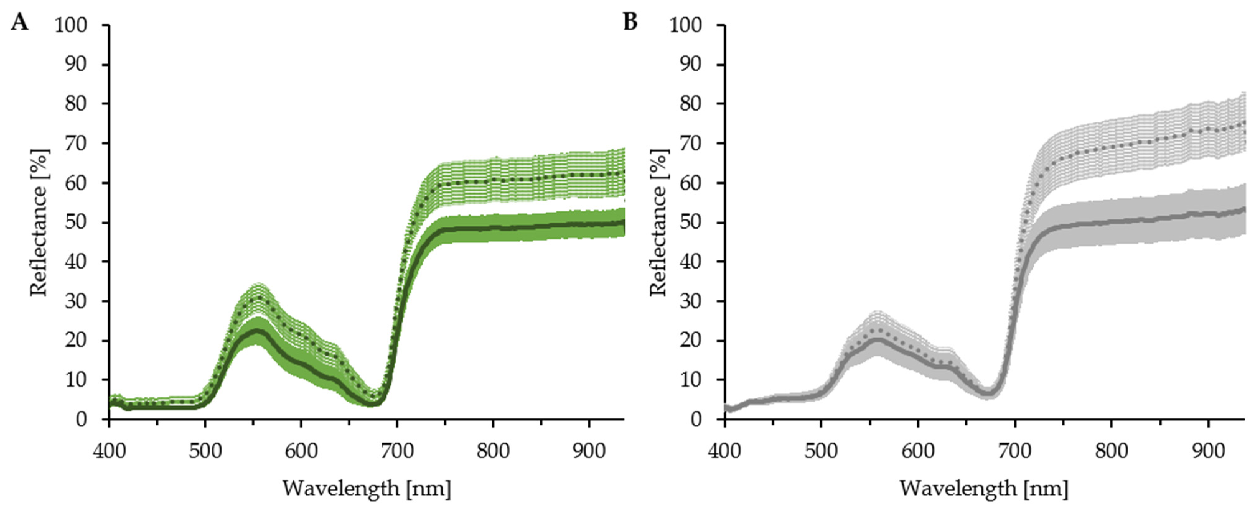
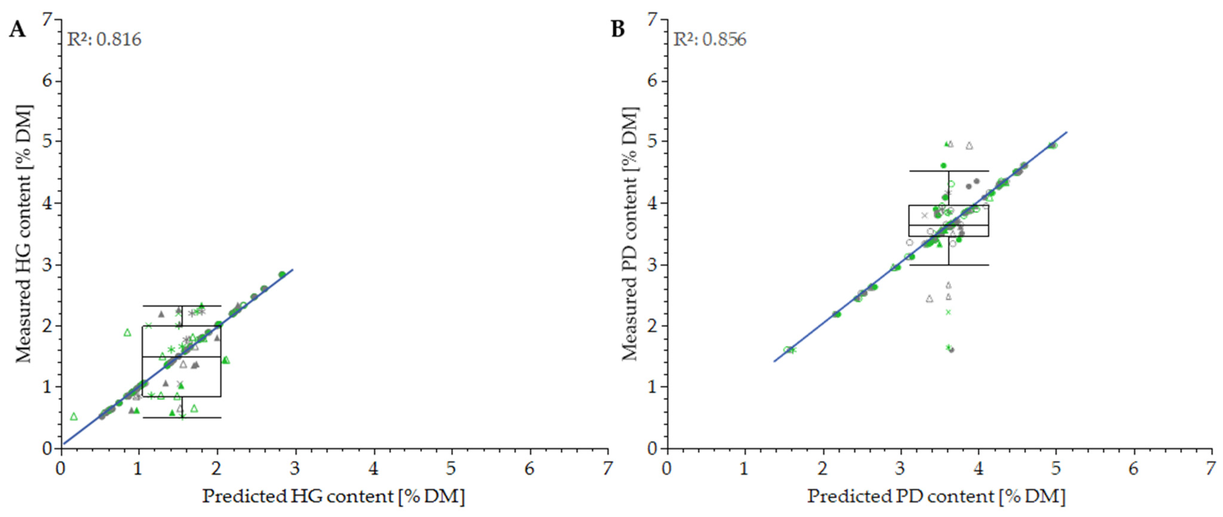
3.3. Impact of Measurement Conditions

For the transferability and replicability of the models for tea-hortensia cultivar differentiation as well as HG or PD assessment, the influence of the measurement background and leaf water status were investigated. While the reflectance spectra of ‘Oamacha’ (Figure 4) showed obvious differences in curve structure, the influence of leaf water status and background color on calculated regressions was negligible. The background color influenced the shape of reflectance spectra in tea-hortensia cultivar ‘Oamacha’, with a higher reflectance on white backgrounds in comparison to black ones for both fresh and dried leaves. In the range from 400 to 700 nm, the effects of measurement background were more pronounced for fresh leaves than for dried leaves. Contrarily, in the red-edge region until 1000 nm, the differences were larger for dried leaves.
The linear regression for ‘Oamacha’ samples is depicted in Figure 5. The training data were reproduced most accurately but for validation samples, the prediction did not appear satisfactory. The Rp2 value was 0.253 and 0.935 for HG and PD, respectively. As no differences between the measurement conditions could be observed between the models, discriminant analysis was conducted. Measurement conditions seemed to not have an important impact on model predictions. For ‘Oamacha’, the discriminant analysis on black and white measurement backgrounds showed that 62% of HG model predictions and 50% of PD model predictions were grouped correctly. For the leaf water status, fresh or dried leaves, 54% of HG predictions, but 75% of PD predictions, were performed correctly. Based on this data, only leaf water status seems relevant in PD modelling. Contrarily, for ‘Amagi Amacha’, 46% of the fresh and dried leaves were grouped correctly, while 73% of the predicted PD values were classified correctly in terms of the background color. For ‘Odoriko Amacha’, 69% and 54% of PD predictions were classified correctly with regard to the measurement background and leaf water status, respectively.

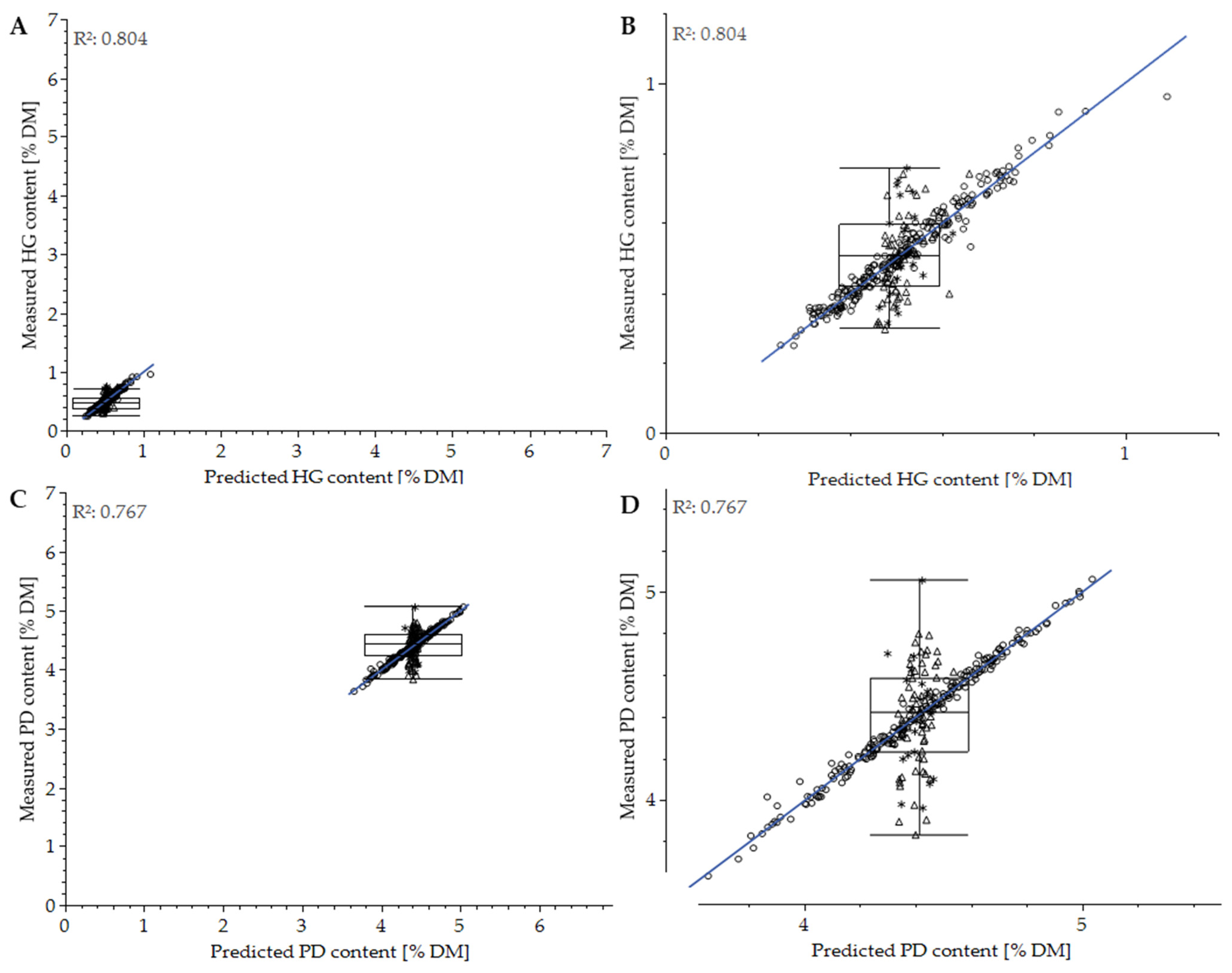
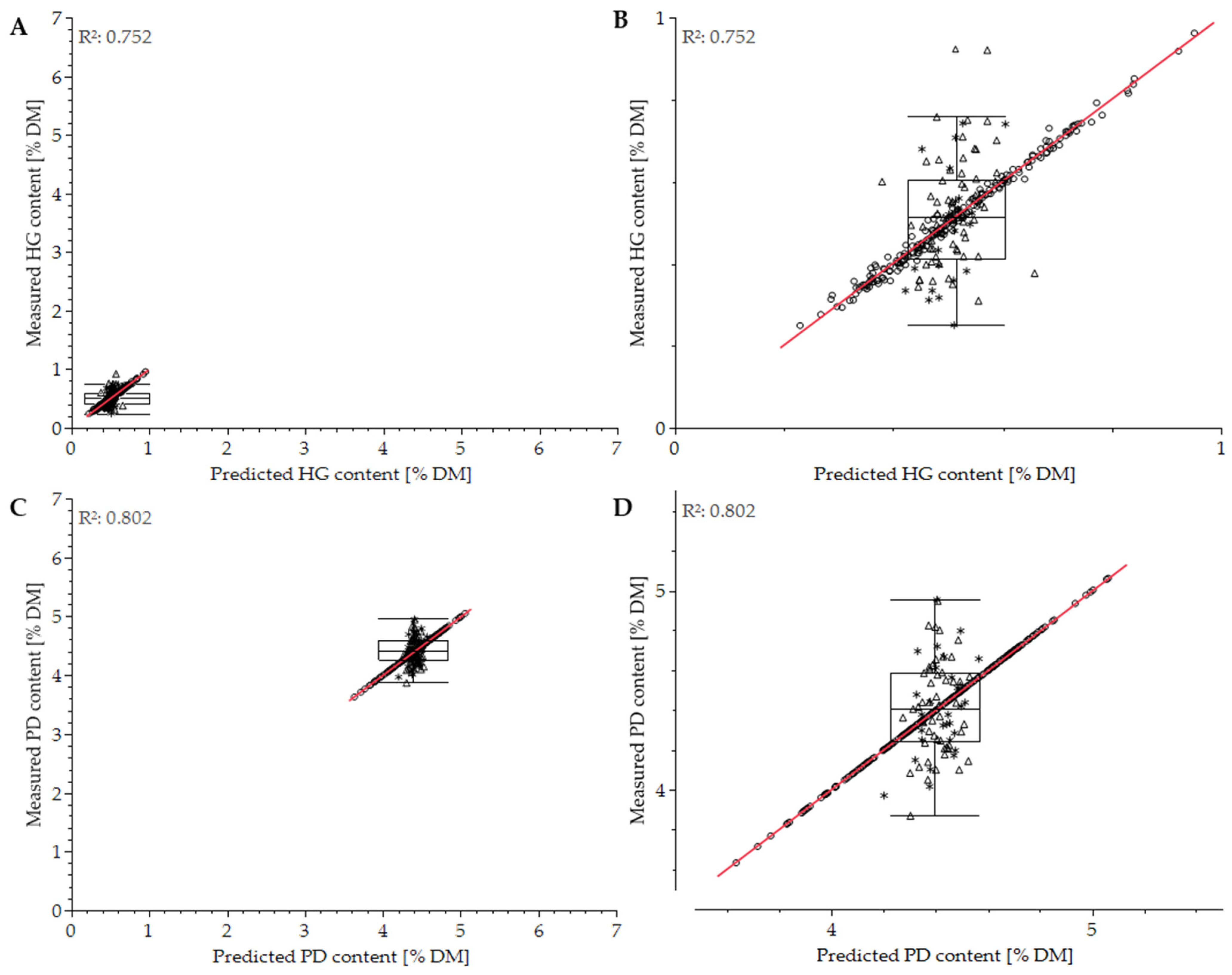
3.4. Effect of Spectrometer

After the differentiation of cultivars appeared to be feasible and the measurement conditions did not seem particularly influential on modeling, the experiment (2021) continued with a larger data set of in-field plants of ‘Oamacha’ using fresh leaf samples and a black measurement background. The aim was to generate models with reflectance spectra recorded by three different spectrometers and to gain a deeper understanding of wavelengths relevant for PLSR.
HG and PD showed great consistency concerning the VIP wavelengths of the reflectance recorded by the Ocean Insight devices. The range of 530–599 nm and between 697 and 737 nm within the VIS spectrum and the ranges of 940–1470 nm and 1497–1664 nm within the NIR spectrum were relevant for both compounds. VIP wavelengths relevant only to HG were 400 nm, 115–116 nm, and 616–644 nm. The range between 1470–1497 nm was only relevant to PD (Figure 6).
With external validation, these VIPs could be confirmed for the most part, and in some cases, variables were either added or removed. From here on, the models will be named according to the spectrometer used for data acquisition (‘Red Tide‘ and ‘Flame-NIR’).
In the following sample set, DHC contents were spread across a small range, so a zoomed-in plot of the linear regressions was required. Predictions based on measurements using the two Ocean Insight spectrometers (Red Tide and Flame-NIR, Figure 7 and Figure 8) showed a strong relationship with the reference analytics of the training data. This was also evident from the statistics of the overall model, as the training sets accounted for a large proportion (70%) of the samples. The Rtotal2 (training + validation + test set) was between 0.75 and 0.80 for the two DHCs. The performance of the validation and test sets, on the other hand, was poor, ranging between 0.006 and 0.236 for Rp2. Contents close to the average value were predicted more accurately, while contents differing from this scattered far outside the regression line. The comparison of Rp2 revealed that HG contents were modeled slightly more accurately than PD. Additionally, ‘Flame-NIR’ resulted in a higher Rp2 than ‘Red Tide’. More precisely, ‘Red Tide’ yielded an Rp2 = 0.105 with an RMSEP of 0.121 and an Rp2 = 0.006 with an RMSEP of 0.274 for HG and PD, respectively. ‘Flame-NIR’ resulted in an Rp2 = 0.236 with an RMSEP of 0.127 for HG and an Rp2 = 0.115 with an RMSEP of 0.230 for PD. Modeling with measurements from both Ocean Insight spectrometers at the same time (Red Tide + Flame-NIR) resulted in an Rp = 0.118 for HG. A slightly higher value of Rp = 0.230 was determined for PD. It should be noted that the measured contents showed only little variation, which could have made modeling difficult. Nevertheless, the laboratory DHC contents of the validation and test samples within the 25th to 75th percentiles (box shown) were estimated with a precision of ±0.1% (HG) and ±0.2% (PD) of the dry matter. However, the exact determination of HG and PD on a leaf level did not seem possible.

3.5. Use of Handheld PolyPen RP400

To simulate measurements on the part of a farmer, a handheld device was used as a third device. By using the PolyPen measurements, VIPs could be reduced to a few, but modeling with just these variables was only possible within a specific division of the samples into the three sets (training, validation, and testing) and did not provide reproducible results. The linear regressions of the reference analytics and modeled values are depicted in Figure 9. For the dataset in 2021, ‘PolyPen’ yielded the highest R2 values for both Rtotal2 and Rp2. Modeling of HG resulted in an Rtotal2 = 0.889 with an RMSEtotal of 0.049 and an Rp2 = 0.422 with an RMSEP of 0.096. As with the Ocean Insight spectrometers, the HG contents of the validation and test samples could be determined with an accuracy of nearly ±0.1% within the interquartile range (25th to 75th percentile). For predicted and measured PD values, the Rtotal2 was 0.904 with an RMSEtotal of 0.084 and Rp2 = 0.582 with an RMSEP of 0.104, respectively, with the latter showing the most precise result in 2021. For PD, the prediction accuracy of the validation and test samples within the interquartile range was increased to ±0.1% of the dry matter content. Although the test set consisted of only of five samples, the minimum and maximum contents were included in this, showing a representative random sample. Despite this, the actual spread of the contents (min to max = 1.32%) was reduced by the prediction, explaining only 0.216% of the variability.
To determine whether significantly better models could be generated using the PolyPen, the Rc2, Rv2, and Rp2 as well as the RMSEC, RMSEV and RMSEP of the three spectrometers were compared. In addition, the influence of the proportion of the training set on both parameters was investigated. An overview of the results for the coefficient of regression is shown in Figure 10. For Rp (the test set), significant differences were found between the PolyPen and the Ocean Insight spectrometers with a training data proportion of ≥70%. The mean values for the Rp2 of the PolyPen models were comparatively significantly higher than those of the Red Tide and Flame-NIR models, specifically, 0.624 compared to 0.033 and 0.107, respectively. Moreover, different ratios of the sample sets influenced the coefficient of determination, Rp. The higher the proportion of training data, the higher the Rp2. It was also shown that the variance of R2 increased with an increasing proportion of the training data but was higher overall for the PolyPen. The RMSE (figure not shown) had a lower variance overall, which also tended to increase as the proportion of training increased. As with the Rp2, a significant difference between the handheld device and the other spectrometers was observed for the test set (RMSEP) when using a training proportion of 70%. The RMSEP was lower for the PolyPen. At the same time, modelling with measurements from the handheld device proved to be more error prone. Out of 25 PLSR trials, with the samples divided into 70% training, 20% validation, and 10% testing, a model was successfully built 13 times, compared to 23 models with the Ocean Insight devices.
As models for a single cultivar did not allow for conclusions to be drawn about the exact content of individual leaves, the mean contents of the lab analytics and the predicted values (test set) were used for comparison. As shown in Figure 11, the box plots of the reference analytics from 2021 were well represented by the modelled DHC contents. For both HG and PD, the measured and predicted values agreed to within one decimal place. For HG, differences of 0.002% (Red Tide), 0.012% (Flame-NIR), and 0.038% (PolyPen) of the dry matter content were determined. Modelled PD contents deviated < 1% from the reference analytics, resulting in differences of 0.004% (Red Tide), 0.007% (Flame-NIR), and 0.017% (PolyPen) in the dry matter content. Consequently, the PLSR models established appeared to be suitable in adequately reproducing an average value of sampled in-field plants. Greater discrepancies were found for the measurement conditions and cultivar differentiation models. When using the measurement conditions data, the mean HG content of 1.514% was well modelled (1.472%), whereas the values for PD were on average 0.234% lower than lab contents. The highest variance (0.332%) was observed when comparing the mean values of PD of the cultivar differentiation model, which was due to the unequal distribution of cultivars into training and test samples.

4. Discussion

This experiment investigated the possibilities of hyperspectral modeling for in-field applications. Therefore, known difficulties and restrictions of hyperspectral measurements of field conditions in comparison to laboratory conditions [56] were purposefully taken into account as well. This led to a practical simulation of rapid in-field measurements in combination with model quality for HG and PD. For this purpose, the accurate depiction of mean HG and PD contents via hyperspectral modeling was sufficient.
The UPLC analysis of DHC contents revealed that the three cultivars show distinct patterns of HG and PD contents. ‘Odoriko Amacha’ yielded the highest HG contents and lowest amounts of PD. ‘Amagi Amacha’ expressed an opposite pattern with high contents of PD while yielding the lowest contents of HG. The tea-hortensia cultivar ‘Oamacha’ was the middle-ground in regard to HG and yielded PD contents that were at the same level as the ones in ‘Amagi Amacha’. A similar pattern for these three cultivars was previously found with one key difference, as ‘Amagi Amacha’ yielded significantly higher PD contents than ‘Oamacha’ [4]. This overlap might be due to a known pattern of seasonal changes [3]. Additionally, this pattern of seasonal changes is more pronounced for ‘Amagi Amacha’ than for other cultivars (unpublished data). This overlap is one major factor influencing the cultivar differentiation via hyperspectral modeling. Besides the HG and PD contents, morphological and physiological differences of the three cultivars could lead to the possible differentiation of cultivars. Leaf hairs [57] and leaf wax [58] influence the reflectance and therefore could allow for the distinction of cultivars. Additionally, adaxial and abaxial surfaces influence hyperspectral modeling for chlorophyll [59]. Nitrogen and chlorophyll [60], as well as general nutrient status [61], are common parameters to be modeled. During the interpretation of such VIS-NIR models, two parameters have to be taken into consideration besides the plant morphology, accuracy, and representativity of measurements. UPLC generally performs at a reasonably well accuracy [62], but as the dynamics of hydrangenol and phyllodulcin in leaves of tea hortensias are not clear yet, hyperspectral measurements might weaken the model quality. This could be due to a lack of representativity of point measurements on the leaves or an uneven distribution of dihydroisocoumarins in the leaf.
As the contents of HG and PD in relation to the respective cultivars performed similarly well for both measured and modeled contents, the modeling of HG and PD for the purpose of cultivar differentiation was successful. The results also show that accurate determinations of HG and PD are not possible from the models developed in this study, while the best results were obtained with the hand-held spectrometer (Table 2). Other spectrometers detecting in the UV and short wavelength infrared (SWIR) regions have previously been investigated for the detection of phenolic compounds and reached an R2 = 0.91 for UV and an R2 = 0.99 for SWIR [63]. Based on these results, different spectrometers that cover other spectral ranges or spectrometers that cover smaller ranges, but yield a higher resolution, might lead to more accurate models.
The VIP wavelengths for HG and PD overlap to a large extent. Still, key wavelengths that only yield information for HG or PD were identified. This leads to the assumption that further research in the field of HG and PD modeling could yield more precise models based on lesser wavelengths. The models shown in this study show two important features. At a first glance, the model quality does not allow for the approximation of HG and PD in single plants for the tea-hortensia cultivar ‘Oamacha’. The regression clearly indicates R2 values that show that no relation of measured and modeled constituent contents was achieved. Consequently, the models are not yet feasible to replace the well-established UPLC analysis. The major feature of such models in this study was to give farmers a decision support. The comparison of mean HG and PD values via UPLC, and the models shown in this study, reveal that the Red Tide modeled mean HG and PD were highly accurate in the test set. Hence, the purpose of the models in this study was successfully achieved as the Red Tide models provided a clear overview of HG and PD contents in the field overall. As single plants are not of interest for farmers, this overview is the key feature necessary for harvest date decisions. The quality of models might also be negatively influenced by the heterogeneity of the plant material. This phenomenon would be ever-present for such applications and is therefore considered for HG and PD models for farmers’ applications.
The results of this study indicate that it is possible to differentiate tea-hortensia cultivars via hyperspectral modeling. Parallelly, the approximation of the mean HG and PD contents were successful as well. Based on these results, further research regarding in-field measurements with more cultivars under different environments and stages during the production cycle are needed. Also, the implementation of spectrometers covering different wavelengths could improve model quality. This would enable more precise applications for research surrounding tea hortensias. Especially breeding and the faster selection based on the HG and PD contents would benefit from accurate models. For in-field cultivation, the incorporation of UAVs presents further improvements, as the detection of wavelengths for multiple plants could be performed in one flight.

5. Conclusions

Chemical analysis of HG and PD are not a sufficient option for farmers to determine optimal harvest dates. Three different spectrometers were investigated for their suitability to model HG and PD contents in three different tea-hortensia cultivars (‘Amagi Amacha’, ‘Oamacha’, and ‘Odoriko Amacha’). Special focus was put on the feasibility and robustness of spectrometer setups for a farm-based application. The differentiation of cultivars based on model predictions showed to be as accurate as predictions based on the actual HG and PD contents, while the effect of measurement background as well as leaf water status (fresh or dried) seems negligible for such applications. Model quality for all three spectrometers tested did not provide a sufficient accuracy to predict HG and PD for lab applications. Still, the models allow for an estimation of mean HG and PD contents on a field scale to give farmers an indication for higher or lower DHC contents to support decision making with regard to harvest dates.

Supplementary Materials

The following supporting information can be downloaded at: https://www.mdpi.com/article/10.3390/horticulturae8030264/s1, Table S1: raw data from 2019; Table S2: raw data from 2021 (Red-Tide and Flame NIR spectrometer); Table S3: raw data from 2021 (PolyPen spectrometer).

Author Contributions

Conceptualization, M.D.M., L.K., E.G. and T.K.; methodology, M.D.M., L.K., E.G., M.B. and T.K.; software, M.D.M., L.K. and E.G.; validation, M.D.M., L.K., E.G. and T.K.; formal analysis, M.D.M., L.K., E.G. and T.K.; investigation, M.D.M., L.K., E.G., M.B. and T.K.; resources, E.-C.S., S.H., J.L. and R.P.; data curation, M.D.M., L.K. and E.G.; writing—original draft preparation, M.D.M. and L.K.; writing—review and editing, E.G., E.-C.S., M.B., S.H., J.L., T.K. and R.P.; visualization, M.D.M., L.K., E.G. and T.K.; supervision, S.H., J.L., T.K. and R.P.; project administration, S.H., J.L., T.K. and R.P.; funding acquisition, J.L. and R.P. All authors have read and agreed to the published version of the manuscript.

Funding

This research was funded by BMEL via Fachagentur Nachwachsende Rohstoffe e.V. (FNR), grant number 22022617.

Data Availability Statement

The data presented in this study are available in the tables or Supplementary Materials.

Acknowledgments

The authors would like to thank Kühne Jungpflanzen, Claus Kühne, and Kötterheinrich Hortensienkulturen e.K. for providing the plant material for this experiment as well as Volker Kraft for additional support regarding JMP Pro 16.

Conflicts of Interest

The authors declare no conflict of interest. The funders had no role in the design of the study; in the collection, analyses, or interpretation of data; in the writing of the manuscript, or in the decision to publish the results.

References

  1. Kindl, H. Formation of a Stilbene in Isolated Chloroplasts. Hoppy Seylers Z. Physiol. Chem. 1971, 325, 767–768. [Google Scholar]
  2. Yagi, A.; Ogata, Y.; Yamauchi, T.; Nishoka, I. Metabolism of Phenylpropanoids in Hydrangea serrata var. thunbergii and the Biosynthesis of Phyllodulcin. Phytochemistry 1977, 16, 1098–1100. [Google Scholar] [CrossRef]
  3. Ujihara, M.; Shinozaki, M.; Kato, M. Accumulation of Phyllodulcin in Sweet-Leaf Plants of Hydrangea serrata and Its Neutrality in the Defence against a Specialist Leafmining Herbivore. Res. Popul. Ecol. 1995, 37, 249–257. [Google Scholar] [CrossRef]
  4. Moll, M.D.; Vieregge, A.S.; Wiesbaum, C.; Blings, M.; Vana, F.; Hillebrand, S.; Ley, J.; Kraska, T.; Pude, R. Dihydroisocoumarin Content and Phenotyping of Hydrangea macrophylla subsp. serrata Cultivars under Different Shading Regimes. Agronomy 2021, 11, 1743. [Google Scholar] [CrossRef]
  5. Suzuki, H.; Ikeda, T.; Matsumoto, T.; Noguchi, M. Polyphenol Components in Cultured Cells of Amacha (Hydrangea macrophylla seringe var. thunbergii Makino). Agric. Biol. Chem. 1978, 42, 1133–1137. [Google Scholar] [CrossRef]
  6. Shin, W.; Kim, S.J.; Shin, J.M.; Kim, S.H. Structure-taste correlations in sweet dihydrochalcone, sweet dihydroisocoumarin, and bitter flavone compounds. J. Med. Chem. 1995, 38, 4325–4331. [Google Scholar] [CrossRef]
  7. Asen, S.; Cathey, H.M.; Stuart, N.W. Enhancement of Gibberellin Growth-Promoting Activity by Hydrangenol Isolated From Leaves of Hydrangea macrophylla. Plant Physiol. 1960, 35, 816–819. [Google Scholar] [CrossRef] [Green Version]
  8. Nozawa, K.; Yamada, M.; Tsuda, Y.; Kawai, K.-I.; Nakajima, S. Antifungal Activity of Oosponol, Oospolactone, Phyllodulcin, Hydrangenol, and Some Other Related Compounds. Chem. Pharm. Bull. 1981, 29, 2689–2691. [Google Scholar] [CrossRef] [Green Version]
  9. Kakegawa, H.; Matsumoto, H.; Satoh, T. Inhibitory Effects of Hydrangenol Derivatives on the Activation of Hyaluronidase and ther Antiallergic Ectivities. Planta Med. 1988, 385–389. [Google Scholar] [CrossRef]
  10. Kim, H.-J.; Kang, C.-H.; Jayasooriya, R.G.P.T.; Dilshara, M.G.; Lee, S.; Choi, Y.H.; Seo, Y.T.; Kim, G.-Y. Hydrangenol inhibits lipopolysaccharide-induced nitric oxide production in BV2 microglial cells by suppressing the NF-κB pathway and activating the Nrf2-mediated HO-1 pathway. Int. Immunopharmacol. 2016, 35, 61–69. [Google Scholar] [CrossRef]
  11. Shin, S.-S.; Ko, M.-C.; Park, Y.-J.; Hwang, B.; Park, S.L.; Kim, W.-J.; Moon, S.-K. Hydrangenol inhibits the proliferation, migration, and invasion of EJ bladder cancer cells via p21WAF1-mediated G1-phase cell cycle arrest, p38 MAPK activation, and reduction in Sp-1-induced MMP-9 expression. EXCLI J. 2018, 17, 531–543. [Google Scholar] [CrossRef] [PubMed]
  12. Myung, D.-B.; Han, H.-S.; Shin, J.-S.; Park, J.Y.; Hwang, H.J.; Kim, H.J.; Ahn, H.S.; Lee, S.H.; Lee, K.-T. Hydrangenol Isolated from the Leaves of Hydrangea serrata Attenuates Wrinkle Formation and Repairs Skin Moisture in UVB-Irradiated Hairless Mice. Nutrients 2019, 11, 2354. [Google Scholar] [CrossRef] [Green Version]
  13. Sanjeewani, W.C.; Sutharsan, S.; Srikrishnah, S. Effects of Hydrangea (Hydrangea macrophylla L.) Leaf Extract Foliar Application on Growth and Yield of Mungbean (Vigna radiata L.). Int. J. Bot. Stud. 2019, 4, 180–184. [Google Scholar]
  14. Nakajima, S.; Sugiyama, S.; Suto, M. Synthesis of Antifungal Isocoumarins (I). Org. Prep. Proced. Int. 1979, 11, 77–86. [Google Scholar] [CrossRef]
  15. Yamahara, J.; Matsuda, H.; Shimoda, H.; Ishikawa, H.; Kawamori, S.; Wariishi, N.; Harada, E.; Murakami, N.; Yoshikawa, M. Development of bioactive functions in hydrangeae dulcis folium. II. Antiulcer, antiallergy, and cholagoic effects of the extract from hydrangeae dulcis folium. Yakugaku Zasshi 1994, 114, 401–413. [Google Scholar] [CrossRef] [PubMed] [Green Version]
  16. Braca, A.; Bader, A.; de Tommasi, N. Plant and Fungi 3,4-Dihydroisocoumarins: Structures, Biological Activity, and Taxonomic Relationships. In Studies in Natural Products Chemistry; Elsevier: Amsterdam, The Netherlands, 2012; Volume 37, pp. 191–215. ISBN 978-0-44459-514-0. [Google Scholar]
  17. Dilshara, M.G.; Jayasooriya, R.G.P.T.; Lee, S.; Jeong, J.B.; Seo, Y.T.; Choi, Y.H.; Jeong, J.-W.; Jang, Y.P.; Jeong, Y.-K.; Kim, G.-Y. Water extract of processed Hydrangea macrophylla (Thunb.) Ser. leaf attenuates the expression of pro-inflammatory mediators by suppressing Akt-mediated NF-κB activation. Environ. Toxicol. Pharmacol. 2013, 35, 311–319. [Google Scholar] [CrossRef] [PubMed]
  18. Kawamura, M.; Kagata, M.; Masaki, E.; Nishi, H. Phyllodulcin, a Constituent of “Amacha”, Inhibits Phosphodiesterase in Bovine Adrenocortical Cells. Pharmacol. Toxicol. 2002, 90, 106–108. [Google Scholar] [CrossRef] [PubMed]
  19. Kim, E.; Lim, S.M.; Kim, M.S.; Yoo, S.H.; Kim, Y. Phyllodulcin, a Natural Sweetener, Regulates Obesity-Related Metabolic Changes and Fat Browning-Related Genes of Subcutaneous White Adipose Tissue in High-Fat Diet-Induced Obese Mice. Nutrients 2017, 9, 1049. [Google Scholar] [CrossRef]
  20. Kim, E.; Shin, J.H.; Seok, P.R.; Kim, M.S.; Yoo, S.H.; Kim, Y. Phyllodulcin, a natural functional sweetener, improves diabetic metabolic changes by regulating hepatic lipogenesis, inflammation, oxidative stress, fibrosis, and gluconeogenesis in db/db mice. J. Funct. Foods 2018, 42, 1–11. [Google Scholar] [CrossRef]
  21. Kamei, K.; Matsuoka, H.; Furuhata, S.I.; Fujisaki, R.I.; Kawakami, T.; Mogi, S.; Yoshihara, H.; Aoki, N.; Ishii, A.; Shibuya, T. Anti-Malarial Activity of Leaf-Extract of Hydrangea macrophylla, a Common Japanese Plant. Acta Med. Okayama 2000, 54, 227–232. [Google Scholar] [CrossRef]
  22. Hu, C.-L.; Ge, L.; Tang, Y.; Li, J.; Wu, C.-H.; Hu, J.-H.; Yuan, J.-T.; Fan, Y.-Z. Phyllodulcin Protects PC12 Cells against the Injury Induced by Oxygen and Glucose Deprivation-Restoration. Acta Pol. Pharm. Drug Res. 2019, 76, 1043–1050. [Google Scholar] [CrossRef]
  23. Swartz, M.E. UPLC™: An Introduction and Review. J. Liq. Chromatogr. Relat. Technol. 2005, 28, 1253–1263. [Google Scholar] [CrossRef]
  24. Nováková, L.; Matysová, L.; Solich, P. Advantages of application of UPLC in pharmaceutical analysis. Talanta 2006, 68, 908–918. [Google Scholar] [CrossRef] [PubMed]
  25. Kumar, A.; Saini, G.; Nair, A.; Sharma, R. UPLC: A Preeminent Technique In Pharmaceutical Analysis. Acta Pol. Pharm. Drug Res. 2012, 69, 371–380. [Google Scholar]
  26. Cozzolino, D. Near infrared spectroscopy in natural products analysis. Planta Med. 2009, 75, 746–756. [Google Scholar] [CrossRef] [Green Version]
  27. Schulz, H. Analysis of Coffee, Tea, Cocoa, Tobacco, Spices, Medicinal and Aromatic Plants, and Related Products. In Near-Infrared Spectroscopy in Agriculture; Roberts, C.A., Ed.; Wiley: Hoboken, NJ, USA, 2004; pp. 345–376. [Google Scholar]
  28. Giovenzana, V.; Beghi, R.; Buratti, S.; Civelli, R.; Guidetti, R. Monitoring of fresh-cut Valerianella locusta Laterr. shelf life by electronic nose and VIS-NIR spectroscopy. Talanta 2014, 120, 368–375. [Google Scholar] [CrossRef]
  29. Ercioglu, E.; Velioglu, H.M.; Boyaci, I.H. Chemometric Evaluation of Discrimination of Aromatic Plants by Using NIRS, LIBS. Food Anal. Methods 2018, 11, 1656–1667. [Google Scholar] [CrossRef]
  30. Wulandari, L.; Permana, B.D.; Kristiningrum, N. Determination of Total Flavonoid Content in Medicinal Plant Leaves Powder Using Infrared Spectroscopy and Chemometrics. Indones. J. Chem. 2020, 20, 1044–1051. [Google Scholar] [CrossRef]
  31. Ercioglu, E.; Velioglu, H.M.; Boyaci, I.H. Determination of terpenoid contents of aromatic plants using NIRS. Talanta 2018, 178, 716–721. [Google Scholar] [CrossRef]
  32. Schulz, H.; Drews, H.-H.; Krüger, H. Rapid NIRS Determination of Quality Parameters in Leaves and Isolated Essential Oils of Mentha Species. J. Essent. Oil Res. 1999, 11, 185–190. [Google Scholar] [CrossRef]
  33. Noland, R.L.; Wells, M.S.; Coulter, J.A.; Tiede, T.; Baker, J.M.; Martinson, K.L.; Sheaffer, C.C. Estimating alfalfa yield and nutritive value using remote sensing and air temperature. Field Crops Res. 2018, 222, 189–196. [Google Scholar] [CrossRef]
  34. Pantazi, X.E.; Moshou, D.; Alexandridis, T.; Whetton, R.L.; Mouazen, A.M. Wheat yield prediction using machine learning and advanced sensing techniques. Comput. Electron. Agric. 2016, 121, 57–65. [Google Scholar] [CrossRef]
  35. Stroppiana, D.; Migliazzi, M.; Chiarabini, V.; Crema, A.; Musanti, M.; Franchino, C.; Villa, P. Rice Yield Estimation Using Multispectral Data From UAV: A Preliminary Experiment In Northern Italy. In Proceedings of the International Geoscience and Remote Sensing Symposium (IGARSS), Milan, Italy, 26–31 July 2015; pp. 4664–4667. [Google Scholar]
  36. Landgrebe, D. On Information Extraction Principles for Hyperspectral Data: A White Paper; School of Electrical and Computer Engineering, Purdue University: West Lafayette, IN, USA, 1997. [Google Scholar]
  37. Famili, A.; Shen, W.-M.; Weber, R.; Simoudis, E. Data Preprocessing and Intelligent Data Analysis. Intell. Data Anal. 1997, 1, 3–23. [Google Scholar] [CrossRef] [Green Version]
  38. Aguilera-Morillo, M.C.; Aguilera, A.M. P-spline Estimation of Functional Classification Methods for Improving the Quality in the Food Industry. Commun. Stat. B Simul. Comput. 2015, 44, 2513–2534. [Google Scholar] [CrossRef]
  39. Aguilera, A.M.; Aguilera-Morillo, M.C. Comparative study of different B-spline approaches for functional data. Math. Comput. Model. 2013, 58, 1568–1579. [Google Scholar] [CrossRef]
  40. Haaland, D.M.; Thomas, E.V. Partial least-squares methods for spectral analyses. 1. Relation to other quantitative calibration methods and the extraction of qualitative information. Anal. Chem. 1988, 60, 1193–1202. [Google Scholar] [CrossRef]
  41. Hotelling, H. The Generalization of Student’s Ratio. Ann. Math. Stat. 1931, 2, 360–378. [Google Scholar] [CrossRef]
  42. Barnes, R.J.; Dhanoa, M.S.; Lister, S.J. Standard Normal Variate Transformation and De-Trending of Near-Infrared Diffuse Reflectance Spectra. Appl. Spectrosc. 1989, 43, 772–777. [Google Scholar] [CrossRef]
  43. Barak, P. Smoothing and Differentiation by an Adaptive-Degree Polynomial Filter. Anal. Chem. 1995, 67, 2758–2762. [Google Scholar] [CrossRef]
  44. Savitzky, A.; Golay, M. Smoothing and Differentiation of Data by Simplified Least Squares Procedures. Anal. Chem. 1964, 36, 1627–1639. [Google Scholar] [CrossRef]
  45. Luo, J.; Ying, K.; He, P.; Bai, J. Properties of Savitzky–Golay digital differentiators. Digit. Signal Process. 2005, 15, 122–136. [Google Scholar] [CrossRef]
  46. O’Haver, T.C. Potential Clinical Applications of Derivative and Wavelength-Modulation Spectrometry. Clin. Chem. 1979, 25, 1548–1553. [Google Scholar] [CrossRef]
  47. Barbin, D.F.; ElMasry, G.; Sun, D.-W.; Allen, P. Predicting quality and sensory attributes of pork using near-infrared hyperspectral imaging. Anal. Chim. Acta 2012, 719, 30–42. [Google Scholar] [CrossRef] [PubMed]
  48. Aleixandre-Tudo, J.L.; Nieuwoudt, H.; Aleixandre, J.L.; Du Toit, W.J. Robust Ultraviolet-Visible (UV-Vis) Partial Least-Squares (PLS) Models for Tannin Quantification in Red Wine. J. Agric. Food Chem. 2015, 63, 1088–1098. [Google Scholar] [CrossRef]
  49. Huang, Y.; Dong, W.; Sanaeifar, A.; Wang, X.; Luo, W.; Zhan, B.; Liu, X.; Li, R.; Zhang, H.; Li, X. Development of simple identification models for four main catechins and caffeine in fresh green tea leaf based on visible and near-infrared spectroscopy. Comput. Electron. Agric. 2020, 173, 105388. [Google Scholar] [CrossRef]
  50. Sanaeifar, A.; Huang, X.; Chen, M.; Zhao, Z.; Ji, Y.; Li, X.; He, Y.; Zhu, Y.; Chen, X.; Yu, X. Nondestructive monitoring of polyphenols and caffeine during green tea processing using Vis-NIR spectroscopy. Food Sci. Nutr. 2020, 8, 5860–5874. [Google Scholar] [CrossRef] [PubMed]
  51. Wold, S.; Sjöström, M.; Eriksson, L. PLS-regression: A basic tool of chemometrics. Chemom. Intell. Lab. Syst. 2001, 58, 109–130. [Google Scholar] [CrossRef]
  52. Dunn, W.J.; Wold, S.; Edlund, U.; Hellberg, S.; Gasteiger, J. Multivariate structure-activity relationships between data from a battery of biological tests and an ensemble of structure descriptors: The PLS method. Quant. Struct. Act. Relat. 1984, 3, 131–137. [Google Scholar] [CrossRef]
  53. Geladi, P.; Kowalski, B.R. Partial least-squares regression: A tutorial. Anal. Chim. Acta 1986, 185, 1–17. [Google Scholar] [CrossRef]
  54. Hu, Y.; Zhang, H.; Liang, W.; Xu, P.; Lou, K.; Pu, J. Rapid and Simultaneous Measurement of Praeruptorin A, Praeruptorin B, Praeruptorin E, and Moisture Contents in Peucedani Radix Using Near-Infrared Spectroscopy and Chemometrics. J. AOAC Int. 2020, 103, 504–512. [Google Scholar] [CrossRef]
  55. Wold, S.; Johansson, E.; Cocchi, M. PLS: Partial least squares projections to latent structures. In 3D QSAR in Drug Design: Theory, Methods and Applications; Kubinyi, H., Ed.; ESCOM: Leiden, The Netherlands, 1993; pp. 523–550. ISBN 90-72199-14-6. [Google Scholar]
  56. Udelhoven, T.; Jarmer, T.; Hostert, P.; Hill, J. The aquisition of spectral reflectance measurements under field and laboratory conditions as support for hyperspectral applications in precision farming. In Proceedings of the 2nd EARSeL Workshop on Imaging Spectroscopy Co-Organized with the SIG “Imaging Spectroscopy”, Enschede, The Netherlands, 11–13 July 2000. [Google Scholar]
  57. Ge, H.; Lu, S.; Zhao, Y. Effects of Leaf Hair on Leaf Reflectance and Hyperspectral Vegetation Indices. Spectrosc. Spec. Anal. 2012, 32, 439–444. [Google Scholar]
  58. Lu, S. Effects of Leaf Surface Wax on Leaf Spectrum and Hyperspectral Vegetation Indices. In Proceedings of the International Geoscience and Remote Sensing Symposium IGARSS 2013, Melbourne, Australia, 21–26 July 2013. [Google Scholar]
  59. Lu, X.; Lu, S. Effects of adaxial and abaxial surface on the estimation of leaf chlorophyll content using hyperspectral vegetation indices. Int. J. Remote Sens. 2015, 36, 1447–1469. [Google Scholar] [CrossRef]
  60. Yamashita, H.; Sonobe, R.; Hirono, Y.; Morita, A.; Ikka, T. Dissection of hyperspectral reflectance to estimate nitrogen and chlorophyll contents in tea leaves based on machine learning algorithms. Sci. Rep. 2020, 10, 17360. [Google Scholar] [CrossRef] [PubMed]
  61. Gong, P.; Pu, R.; Heald, R.C. Analysis of in situ hyperspectral data for nutrient estimation of giant sequoia. Int. J. Remote Sens. 2002, 23, 1827–1850. [Google Scholar] [CrossRef]
  62. Saviano, A.M.; Madruga, R.O.G.; Lourenço, F.R. Measurement uncertainty of a UPLC stability indicating method for determination of linezolid in dosage forms. Measurement 2015, 59, 1–8. [Google Scholar] [CrossRef]
  63. Tschannerl, J.; Ren, J.; Jack, F.; Krause, J.; Zhao, H.; Huang, W.; Marshall, S. Potential of UV and SWIR hyperspectral imaging for determination of levels of phenolic flavour compounds in peated barley malt. Food Chem. 2019, 270, 105–112. [Google Scholar] [CrossRef] [Green Version]
Figure 1. Hydrangenol (HG) and phyllodulcin (PD) contents of three tea-hortensia cultivars harvested on 9 July 2019 (trial 2019) and 20 August 2021 (trial 2021 I and trial 2021 II). Trial 2021 I represents data used for modeling based on the Ocean Insight spectrometers, while trial 2021 II indicates HG and PD contents for modeling the PolyPen data. The differences in data used for the models in 2021 occur according to the data preprocessing described in Section 2—Material and Methods. Significant differences were determined by ANOVA and Tukey-HSD as post-hoc procedure (p = 0.05) and are indicated by letters (ac) for 2019, while trials in 2021 were investigated by t-test (p = 0.05), differences were not significant (ns).
Horticulturae 08 00264 g001
Figure 2. Averaged raw spectra of H. macrophylla subsp. serrata cutivars (green: ‘Oamacha’ (n = 40), orange: ‘Odoriko Amacha’ (n = 40), and purple: ‘Amagi Amacha’ (n = 35)) measured with the Red Tide spectrometer in 2019 using fresh leaf samples and a black measuring background. (A) shows the averaged spectra while (BD) show the average value ± SD of the respective cultivar.
Horticulturae 08 00264 g002
Figure 3. Regression of predicted and measured (Red Tide, 2019) contents of (A) HG and (B) PD for the three tea-hortensia cultivars (purple: ‘Amagi Amacha’, green: ‘Oamacha’, and orange: ‘Odoriko Amacha’) including coefficient of determination. Different symbols indicate the training (o), validation (∆), and test (*) sets (HG: training (n = 86), validation (n = 18), test (n = 11); PD: training (n = 80), validation (n = 26), test (n = 9)).
Horticulturae 08 00264 g003
Figure 4. Averaged raw spectra ± SD (n = 40) of H. macrophylla subsp. serrata ‘Oamacha’ samples measured under different conditions with Red Tide spectrometer in 2019. Green coloring indicates fresh leaves (A), grey coloring indicates dried leaves (B). The continuous lines represent a black measuring background while the hatched lines represent a white measuring background.
Horticulturae 08 00264 g004
Figure 5. Regression of predicted and measured (Red Tide, 2019) contents of (A) HG and (B) PD for H. macrophylla subsp. serrata ‘Oamacha’ including the coefficient of determination. The different symbols indicate the training (o), validation (∆), and test set (*/x) (HG: training (n = 119), validation (n = 28), test (n = 13); PD: training (n = 118), validation (n = 26), test (n = 16). The green coloring indicates fresh leaves and the grey coloring indicates dried leaves. The filled symbols represent a black measuring background (test set: *), while the unfilled symbols represent a white measuring background (test set: x). The boxplots illustrate the variation of the measured DHC contents in the validation and test sets.
Horticulturae 08 00264 g005
Figure 6. Individual raw spectra of ‘Oamacha’ samples (n = 296) measured in 2021 with Ocean Insight spectrometers. Colored ranges indicate the VIP wavelengths using Red Tide (blue) and Flame-NIR (red). Depending on the DHC compound, ranges have different shading (HG: light shade, PD: dark shade, DHC (HG + PD): medium shade).
Horticulturae 08 00264 g006
Figure 7. Regression of predicted and measured (Red Tide, 2021) contents of HG (A,B) and PD (C,D) for H. macrophylla subsp. serrata ‘Oamacha’ including the coefficient of determination and a zoomed-in version (B,D). The different symbols indicate the training (o), validation (∆), and test sets (*) (HG: training (n = 221), validation (n = 50), test (n = 25); PD training (n = 211), validation (n = 64), test (n = 21)). Boxplots illustrate the variation of the measured DHC contents among the validation and test sets.
Horticulturae 08 00264 g007
Figure 8. Regression of the predicted and measured (Flame-NIR, 2021) contents of HG (A,B) and PD (C,D) for H. macrophylla subsp. serrata ‘Oamacha’ including the coefficient of determination and a zoomed-in version (B,D). The different symbols indicate the training (o), validation (∆), and test (*) sets (HG: training (n = 215), validation (n = 57), test (n = 24); PD: training (n = 215), validation (n = 53), test (n = 28)). The boxplots illustrate the variation of the measured DHC contents among the validation- and test set.
Horticulturae 08 00264 g008
Figure 9. Regression of the predicted and measured (PolyPen, 2021) contents of HG (A,B) and PD (C,D) for H. macrophylla subsp. serrata ‘Oamacha’ including coefficient of determination and a zoomed-in version (B,D). The different symbols indicate the training (o), validation (∆), and test (*) sets (HG: training (n = 42), validation (n = 11), test (n = 7); PD: training (n = 43), validation (n = 12), test (n = 5)). The boxplots illustrate the variation of the measured DHC contents among the validation- and test set.
Horticulturae 08 00264 g009
Figure 10. Coefficient of determination (R2) for PLSR models of phyllodulcin (PD) developed using measurements of H. macrophylla subsp. serrata samples in 2021. The different coloring indicates the spectrometers used (blue: Red Tide, red: Flame-NIR, yellow: PolyPen). Letters (ag) represent the different splitting of the sample set (training/validation/test set ratio: (a) = 2/5.3/2.7; (b) = 3/4.7/2.3; (c) = 4/4/2; (d) = 5/3.3/1.7; (e) = 6/2.7/1.3; (f) = 7/2/1; (g) = 8/1.3/0.7). n = 5 except for the letter f (ratio used for modeling): Red Tide n = 23; Flame-NIR n = 23; PolyPen n = 13. Significant differences were determined by ANOVA with the Tukey-HSD test as a post-hoc procedure (p = 0.05) and are indicated by letters (a, ab, b). Letters above the boxplots refer to the differences between the ratios (row) and the letters below the boxplots refer to differences between the spectrometers within a ratio (box).
Horticulturae 08 00264 g010
Figure 11. DHC (HG: hydrangenol, PD: phyllodulcin) contents from chemical analysis via UPLC (filled box) and modeled contents (test set, colorless box) for different models computed and compilated in this study based on the five models shown in this study.
Horticulturae 08 00264 g011
Table 1. Wavelength ranges and preprocessing methods (standard normal variate (SNV) transformation and Savitzky–Golay (SG) filters) used for modeling of hydrangenol (HG) and phyllodulcin (PD).
Spectrometer
(Year of Experiment)
Wavelength Range [nm] for SNV TransformationWavelength Range [nm] for SG FilterPreprocessing Method
(DHC Compound)
Red Tide (2019)350–938360–928SNV + SG smoothing: 5th polynomial order; distance to right/left filter edge = 10 (HG, PD)
Red Tide (2021)350–1000420–918SNV + SG smoothing: 5th polynomial order, distance to right/left filter edge = 20 (HG, PD)
Flame-NIR (2021)940–1664-SNV
Red Tide + Flame-NIR (2021)400–1664-SNV
PolyPen (2021)325–792353–765SNV + SG 2nd derivative: 7th polynomial order; distance to right/left filter edge = 15 (HG)
382–740SNV + SG 1st derivative: 7th polynomial order; distance to right/left filter edge = 30 (PD)
Table 2. Statistical evaluation of the goodness of fit test modeling hydrangenol (HG) and phyllodulcin (PD) including the coefficient of determination (R2) and root mean square error (RMSE) for the the calibration (Rc2/RMSEC), validation (Rv2/RMSEV), and prediction (test) sets (Rp2/RMSEP), as well as the overall model (Rtotal2/RMSEtotal) consisting of all three sets.
ModelDHC CompoundCalibrationValidationPredictionOverall Model
Rc2RMSECRv2RMSEVRp2RMSEPRtotal2RMSEtotal
Cultivar differentiationHG0.9190.5690.9980.0990.9980.1160.9410.496
PD0.9100.3400.8930.3440.9100.3400.9210.305
Measurement conditionsHG1.0000.0070.2390.5230.2530.5490.8160.273
PD0.8610.2610.7620.2970.9350.1960.8560.261
Red Tide 2021HG0.9590.0280.2760.1010.1050.1210.8040.059
PD0.9890.0290.1140.2210.0060.2740.7670.128
Flame-NIR 2021HG0.9890.0140.0870.1240.2360.1270.7520.066
PD1.0000.0010.0240.2290.1150.2300.8020.118
Red Tide + Flame-NIRHG1.0000.0010.1730.1290.1180.1340.7530.066
PD0.9980.0120.0760.2190.2300.2250.8200.112
PolyPen 2021HG0.9910.0150.8630.0620.4220.0960.8890.049
PD0.9980.0150.1940.1820.5820.1040.9040.084
Publisher’s Note: MDPI stays neutral with regard to jurisdictional claims in published maps and institutional affiliations.

