Quality Grading Algorithm of Oudemansiella raphanipes Based on Transfer Learning and MobileNetV2

Abstract

As a traditional edible and medicinal fungus in China, Oudemansiella raphanipes has high economic benefits. In order to achieve the automatic classification of Oudemansiella raphanipes into four quality levels using their image dataset, a quality grading algorithm based on neural network models was proposed. At first, the transfer learning strategy and six typical convolution neural network models, e.g., VGG16, ResNet50, InceptionV3, NasNet-Mobile, EfficientNet, and MobileNetV2, were used to train the datasets. Experiments show that MobileNetV2 has good performance considering both testing accuracy and detection time. MobileNetV2 only needs 37.5 ms to classify an image, which is shorter by 11.76%, 28.57%, 46.42%, 59.45%, and 79.73%, respectively, compared with the classification times of InceptionV3, EfficientNetB0, ResNet50, NasNet-Mobile, and VGG16. Based on the original MobileNetV2 model, four optimization methods, including data augmentation, hyperparameter selecting, an overfitting control strategy, and a dynamic learning rate strategy, were adopted to improve the accuracy. The final classification accuracy can reach as high as 98.75%, while the detection time for one image is only 22.5 ms and the model size is only 16.48 MB. This quality grading algorithm based on an improved MobileNetV2 model is feasible and effective for Oudemansiella raphanipes, satisfying the needs in the production line.

1. Introduction

Oudemansiella raphanipes is one of the traditional Chinese edible and medicinal mushrooms and has high development value [1]. It is not only rich in many nutrients, such as vitamins, amino acids, and rich trace elements, but also has some medical effects, such as anti-inflammatory and analgesic effects. Owing to the significantly different prices in the market for different qualities of Oudemansiella raphanipes, it is very important for quality grading to distinguish the high-quality products from the poor-quality ones. However, the traditional manual quality grading process requires a high labor force and is low in efficiency, which seriously restricts the economic benefits. Therefore, it is urgent to develop an automated and intelligent quality grading algorithm for Oudemansiella raphanipes.

The quality grading of Oudemansiella raphanipes belongs to the field of image classification. In recent years, with the development of deep learning, convolutional neural networks (CNNs) can fully extract the high-dimensional features of objects. The classification algorithm based on deep learning has been widely used for various crops, such as grains [2,3,4], fruits [5,6,7,8], and vegetables [9,10,11]. For instance, Sujatha R et al. compared the performance of machine learning (support vector machine, random forest, stochastic gradient descent) and deep learning (InceptionV3, VGG16, VGG19) in terms of citrus plant disease detection, showing that VGG16 had the best classification accuracy of 89.5% [12]. Esgario J. G. M. et al. estimated the stress severity caused by biotic agents on coffee leaves using ResNet50, showing an accuracy of 95.24% for the biotic stress classification and 86.51% for severity estimation [13]. Arwatchananukul S et al. recognized 15 species of Paphiopedilum orchid using the InceptionV3 feature extractor, showing a recognition rate of up to 98.6% [14]. Ji M. et al. proposed a binary relevance multi-label learning algorithm combined with NasNet to simultaneously recognize 7 crop species, classify 10 crop diseases, and estimate the severity of 3 kinds of crop disease, showing a test accuracy of 85.28% [15]. Suharjito et al. classified the ripeness levels of a fresh fruit bunch of oil palm using EfficientNetB0 with a data augmentation method named “9-angle crop”, showing a good test accuracy of 89.8% on Keras datasets [16].

In terms of the classification of mushrooms, Preechasuk J. et al. detected the 45 species of edible and poisonous mushrooms by a 6-layer CNN with the average accuracy of 74% on the dataset of 8556 images [17]. Zahan N. et al. used InceptionV3, VGG16, and ResNet50 to identify the 45 species of edible, inedible, and poisonous mushrooms, and InceptionV3 achieved the highest accuracy of 88.40% on the dataset of 8190 images [18]. Zhao M. et al. proposed a four-type classification method based on a compound knowledge distillation algorithm, using ResNet50 as the teacher model and ResNet18 as the student model to perform weight training and compound distillation on the dataset of 3000 images, in which the testing accuracy was 96.89% and the detection time was 32 ms [19]. Ketwongsa W. et al. classified five species of edible and poisonous mushrooms based on AlexNet, ResNet50, and GoogleNet, and a proposed modified AlexNet model using a dataset of 623 images; the proposed model had the fastest training time while maintaining an accuracy of 98.5% [20].

In a production line, the quality grading of mushrooms requires not only a high accuracy, but also a small detection time and few computing resources. However, the deep learning CNN often demands a large detection time and a high level of computing resources. MobileNet is the first generation of lightweight neural networks [21] and has demonstrated its high accuracy as well as small detection time and low requirement of computing resources on various datasets [22,23,24,25,26]. Compared with other neural networks [27,28,29,30,31,32,33], the depth separable convolution in MobileNet leads to a smaller number of parameters and, thus, a smaller amount of calculation. As a result, the high accuracy MobileNet can also achieve a fast speed on a CPU and a small storage space, which is suitable for practical industrial computers.

Moreover, the collection of labelled datasets is time-consuming and labor-intensive work; thus, sometimes only a small dataset can be obtained. However, a deep CNN trained from scratch with small datasets has difficulty obtaining high accuracy. As a result, transfer learning was used to obtain knowledge from a big dataset, and then to complete new tasks using small datasets [9].

In this paper, we provide an algorithm for the quality grading of Oudemansiella raphanipes, which is a good case study when developing a new image classification application. At first, six typical CNNs, including VGG16, ResNet50, InceptionV3, NasNet-Mobile, EfficientNet, and MobileNetV2, were pretrained on the dataset of ImageNet and transferred to our dataset of Oudemansiella raphanipes. Balancing the three criterions of high accuracy, small detection time, and small mode size, MobileNetV2 was selected and improved for the quality grading of Oudemansiella raphanipes. The final classification accuracy can reach as high as 98.75%, while the detection time for one image is only 22.5 ms and the model size is only 16.48 MB. This algorithm is efficient, fast, and resource-saving, which meets the demand of the price-sensitive market and is suitable for deployment on the production line.

2. Materials and Methods

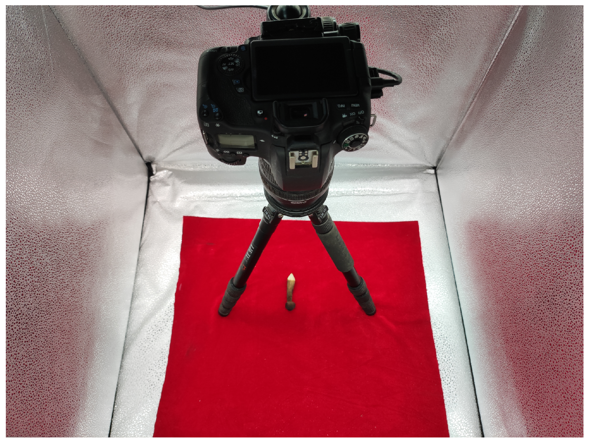
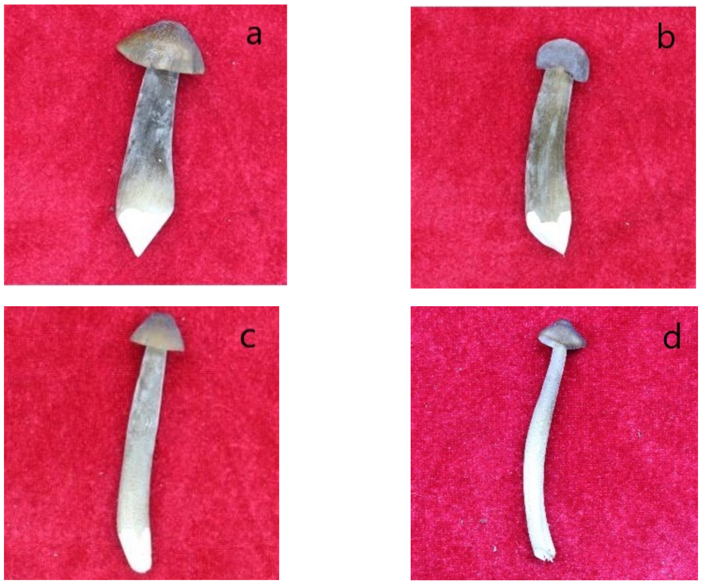
2.1. Datasets

Figure 1 shows our experimental setup for image acquisition. Each Oudemansiella raphanipes was put into a shielding box, in which a light source (four 45-watt fluorescent lamps with a color temperature of 5000 K) was illuminated from the top and a color camera (Canon 760D with EOSUtility software) took the images with the vertical shooting height of 45 cm. The resolution of each image is 3984 × 2656.

All these images were preliminarily labeled by three experts and divided into four quality levels: Class 1, Class 2, Class 3, and Class 4, according to the size, shape, color, texture, viewpoint. After preliminarily labelling, the three experts inspected each category and corrected the wrongly labelled images after discussion. Finally, each category contained 1000 images, the quality level of which was agreed and confirmed by all three experts. Figure 2 gives a typical example of each category.

Before training, the input image needed to be preprocessed. Firstly, the image was downscaled in equal proportion so that it could be used as the input of a neural network. For example, in the MobileNetV2 network [21], the image size needs to be adjusted to be 224 × 224 × 3 pixels. Secondly, the images of each category were randomly grouped into a training dataset, a validation dataset, and a testing dataset at a ratio of 7:2:1. After grouping, there were 2800 images in the training set (700 images for each category), 800 images in the validation set (200 images for each category), and 400 images in the testing set (100 images for each category).

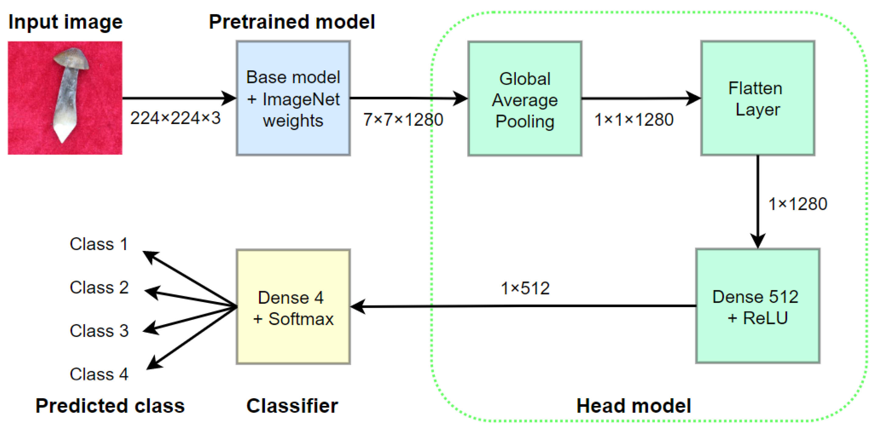
2.2. Transfer Leaning

Figure 3 gives the flowchart of the transfer learning method. At first, the selected base model, e.g., MobileNetV2, was trained on a big dataset, e.g., ImageNet [34], and its network weights were determined. Following the pretrained model, we added a head model and a classifier layer. The head model had a global average pooling layer, a flatten layer, and a fully connected layer. The global average pooling layer was used to down-sample the output of the pretrained model, the flattening layer was used to flatten the multi-dimensional vector into one dimension, and the fully connected layer adopted the ReLU as the activation function to integrate and map the image features into values. The classifier layer adopted the softmax activation function to classify the values’ output from the fully connected layer. Subsequently, the whole model composed of the pretrained model, the head model, and the classifier layer was trained on the small dataset acquired in Section 2.1. Note that the network weights of the pretrained model are kept frozen in the small dataset training, while those of the head model and the classifier layer should be trained.

2.3. Computing Resources

One benefit of transfer leaning is that the required computing resources are less than the traditional CNN training. The computing resources used in this paper are shown in

Table 1. Computing resources.

Equipment	Environment
CPU	Intel(R) Core(TM) i5-8250U, 1.80 GHz
Memory	8 GB
Operation system	Windows 10 (64bit)
Python	Version 3.7.0
Tensorflow	Version 2.3.0
Compiler environment	PyCharm 2020

.

3. Results

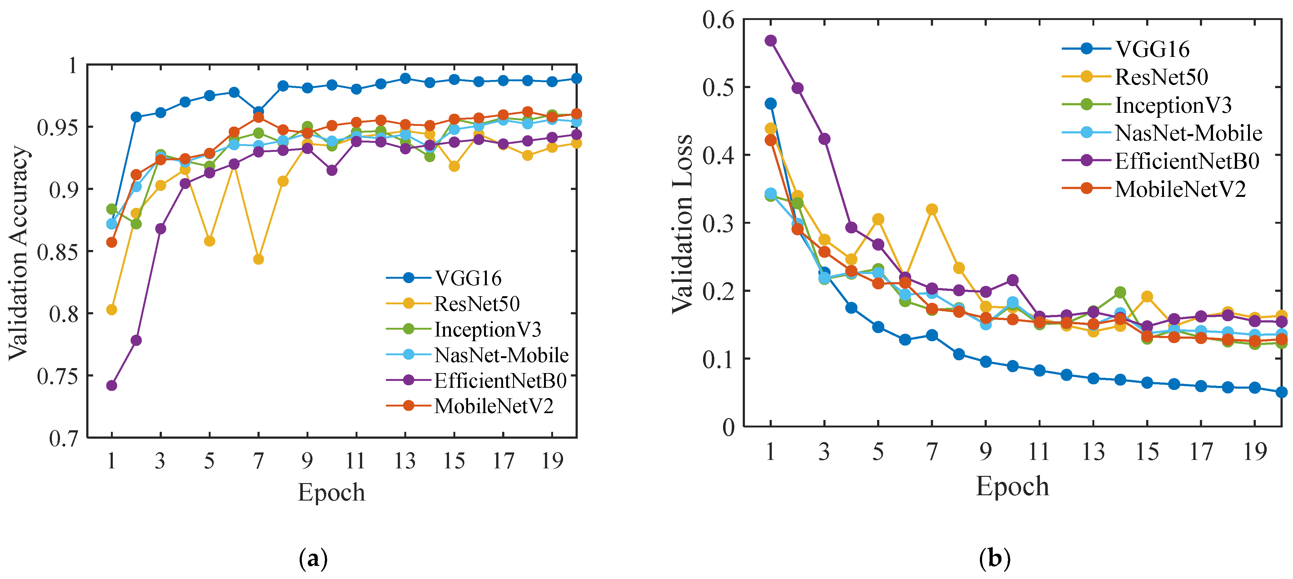
3.1. Comparison of MobileNetV2 with other Five Typical CNN Models

Six typical CNN models, including VGG16 [27], ResNet50 [28], InceptionV3 [29], NasNet-Mobile [30], EfficientNetB0 [31], and MobileNetV2 [21], were evaluated based on the transfer learning from a big dataset, that is, ImageNet [34], to a small dataset, that is, the dataset acquired in Section 2.1.

In the training process, the Adam optimizer was adopted, the learning rate was selected as 0.01, the batch size was 16, and the number of epochs was 20. Figure 4 gives the validation accuracies and losses. VGG16 can reach the highest validation accuracy of 98.88% and the lowest validation loss. ResNet50 fluctuates greatly in the early epochs and its validation accuracy is only 93.68%. EfficientNetB0 also has a relatively lower accuracy of 94.37%. The convergence characteristics of InceptionV3, NasNet-Mobile, and MobileNetV2 are similar, and their validation accuracies are 95.96%, 95.42%, and 96.04%, respectively.

The trained models were applied on the testing dataset and their confusion matrixes are presented in Figure 5. Each of the six CNN models have good recognition accuracies for the four classes, except that there are many errors in the identification of Class 1 from Class 2. It also seems that the classification errors between Class 1 and Class 2 are higher than those between Class 3 and 4. However, the classification errors between the relatively high-quality Oudemansiella raphanipes (Class 1 and 2) and the relatively low-quality ones (Class 3 and 4) is very low, indicating that the characteristics of these two levels of products are obvious and easy to distinguish.

The testing accuracy on the total testing dataset, the average detection time for a single image, and the model size are given in

Table 2. The testing accuracy, average detection time, and model size of VGG16, ResNet50, InceptionV3, NasNet-Mobile, EfficientNetB0, and MobileNetV2.

CNN Models	Test Accuracy (%)	Average Detection Time (ms)	Model Size (MB)
VGG16	97.75	185	56.20
ResNet50	90.00	70	90.38
InceptionV3	94.25	42.5	83.74
NasNet-Mobile	94.25	92.5	23.70
EfficientNetB0	93.00	52.5	23.35
MobileNetV2	94.75	37.5	16.44

. In terms of testing accuracy, VGG16 still performs the best and can reach an accuracy of 97.75%. InceptionV3, NasNet-Mobile, and MobileNetV2 also perform well with accuracies of 94.25%, 94.25%, and 94.75%, respectively, while EfficientNetB0 has a relatively low testing accuracy of 93%. Owing to the errors in the identification of Class 1 (see Figure 5b), ResNet50 has an overall accuracy of only 90%. In terms of detection time, MobileNetV2 only needs 37.5 ms to classify an image, which is lower than that of the other five models. This detection time is shortened by 11.76%, 28.57%, 46.42%, 59.46%, and 79.73%, respectively, compared with those of InceptionV3, EfficientNetB0, ResNet50, NasNet-Mobile, and VGG16. In terms of the size of the model, MobileNetV2, representing a typical lightweight CNN, takes up the least memory space because the number of parameters is much smaller than that of ordinary CNN models. It only needs 16.44 MB of storage space, which is smaller than the 23.35 MB of EfficientNetB0, 23.70 MB of NasNet-Mobile, 56.2 MB of VGG16, 90.38 MB of ResNet50, and 83.74 MB of Inception V3.

In the production line of Oudemansiella raphanipes, the appropriate quality grading algorithm should not only consider the accuracy but also the matching degree of hardware equipment. Although VGG16 performs excellently when testing accuracy, it is not suitable for our grading owing to its long detection time and high requirement of computing resources. ResNet50 performs poorly on the dataset and cannot meet the accuracy requirements. Both InceptionV3 and NasNet-Mobile have a moderate accuracy, but the former requires a large model size, while the latter requires a long detection time. EfficientNetB0 balances the testing accuracy, the detection time, and the model size, but the performance is still not good enough. Compared with the above five models, MobileNetV2 can greatly shorten the detection time and can be deployed in productional computers, or even mobile phones, with poor computing resources, while its accuracy is only 3% lower than that of VGG16. These advantages are in line with the production practice. As a result, we selected MobileNetV2 as the basic model for the following improvements to increase the testing accuracy.

3.2. Optimizations of MobileNetV2

Four optimization methods, including data augmentation, hyperparameter selecting, an overfitting control strategy, and a dynamic learning rate strategy, were applied on the MobileNetV2 model to further improve its classification accuracy while giving full play to the advantages of portability and rapidity. In the experiments, each model was trained three times and the average values of validation accuracies and losses were taken to prevent random errors.

3.2.1. Optimization 1: Data Augmentation

A small amount of training data have difficulty providing enough information for the model to learn. Therefore, data augmentation is often used to expand the amount of data so as to make the model fully learn the image features and to improve the generalization ability of the model.

For our dataset of Oudemansiella raphanipes, three methods, including 90° rotation, horizontal flip, and vertical flip, were randomly used to enrich the dataset. The dataset was expanded to 8000 images. Therefore, we had 5600 images in the training set (1400 images for each category), 1600 images in the verification set (400 images for each category), and 800 images in the testing set (200 images for each category).

3.2.2. Optimization 2: Hyperparameter Selecting

In the training process of a neural network model, the appropriate hyperparameters can effectively accelerate the convergence of the model and improve its accuracy. Based on the basic model after data augmentation, four important hyperparameters, including the optimizer, learning rate, batch size, and number of epochs, were investigated.

• Optimizer

The Adam, SGD, and Adagrad optimizers were investigated. The Adam optimizer performs the best on the validation accuracy and loss.

• Learning Rate

The learning rates of 0.1, 0.01, 0.001, and 0.0001 were evaluated. If the learning rate is 0.001, both the validation accuracy and loss have relatively stable convergence trends, which can not only avoid the large fluctuations when the learning rate is larger, but also avoid the slow convergence speed when the learning rate is smaller.

• Batch Size

The batch sizes of 8, 16, 32, and 64 were examined. A small batch size, such as 8 or 16, leads to a short training time but a significant fluctuation in the function curves of validation accuracy and loss. A large batch size, such as 32 or 64, leads to a stable and fast convergence speed but a relatively long training time. Considering the validation accuracy and training time, the batch size of 32 was adopted.

• Number of Epochs

The number of epochs was set as large as 40 for performance evaluation. The validation accuracy and loss curves decrease rapidly in the first 20 epochs. After that, the curves are convergent, indicating that the performance of the model is no longer improved. Balancing the training time and validation accuracy, the number of epochs was set to 20 in the following experiments.

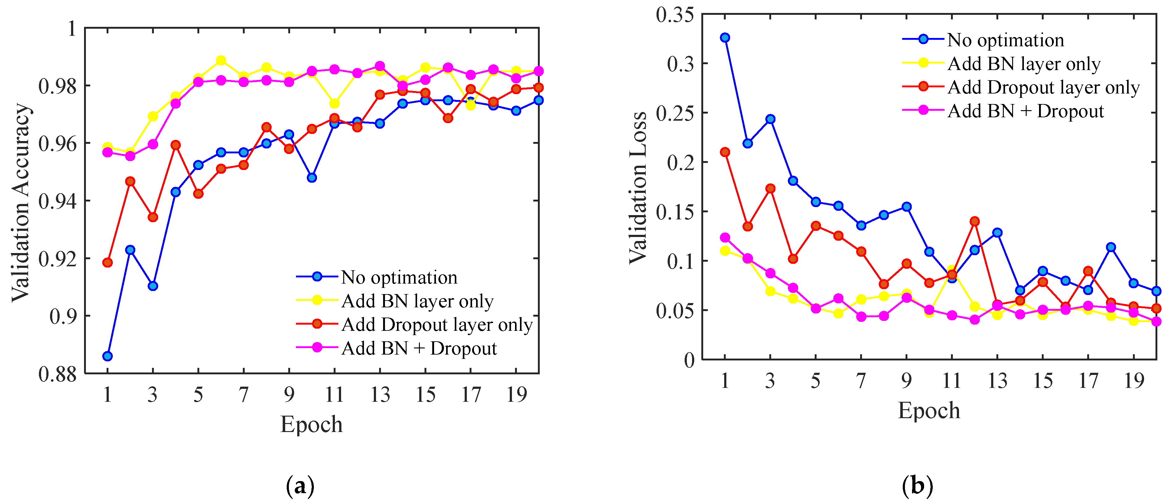
3.2.3. Optimization 3: Overfitting Control Strategy

Overfitting is a condition where the model fits well with the training dataset but does not have good generalization ability, thus it provides low accuracy on new datasets. The appropriate overfitting control strategy can improve the validation and testing accuracies. On the basis of the optimized model after hyperparameter selection, two overfitting control strategies, including the batch normalization (BN) layer [35] and the dropout layer [36], were discussed.

We added the BN layer after the pretrained model to normalize its last convolution layer and the dropout layer after the fully connected layer in the head model. The probability in the dropout layer was set to 0.5, which means that the neuron had a 50% probability of being dropout. Figure 6 presents the validation accuracies and losses of different cases with or without the two strategies. It is shown that adding both the BN and dropout layers can effectively restrain the curve fluctuation and improve the validation accuracy as well as reduce the validation loss. It is better to apply the two strategies simultaneously than to apply only one alone. Compared with the dropout layer, the BN layer plays a more important role in accelerating the convergence speed. In addition, the training accuracy after applying both strategies is 99.02%, while the validation accuracy is 98.50%, with a difference of 0.52%. This value is lower than the difference of 2.18% in the model with optimization 2, proving the effectiveness of the overfitting control strategies.

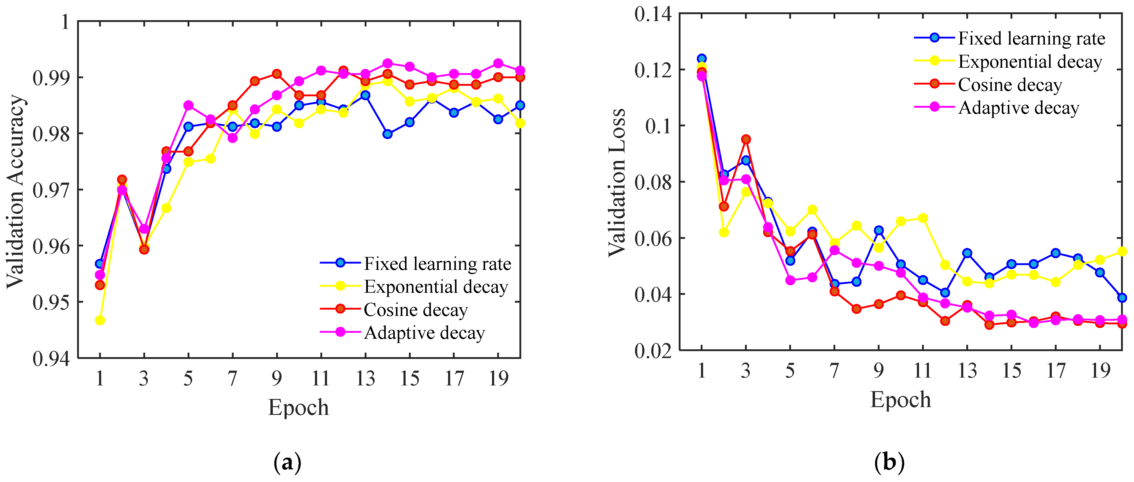
3.2.4. Optimization 4: Dynamic Learning Rate Strategy

Whether the learning rate is good or not depends on two aspects: (a) the convergence speed should be as fast as possible and (b) the optimal solution can be found accurately. From the results in Section 3.2.2 (not shown here), a large learning rate makes the validation loss curve decline rapidly in the early epochs of training, but it also causes fluctuation in the later epochs, which makes it difficult for the model to converge to the optimal solution; a small learning rate makes the validation loss curve more stable in the later epochs, but there is a problem of slow convergence. If both a large learning rate and a small learning rate are combined in the training process to provide the full effect of their respective advantages, the training performance can be further improved. This is the adjustment strategy of the dynamic learning rate. Generally, the dynamic learning rate means that a large learning rate is set in the early epochs of training and is attenuated to be a relatively small value in the later epochs.

Three adjustment strategies, including exponential decay, cosine annealing decay, and adaptive decay, were evaluated.

• Exponential Decay

Exponential decay obeys ${\alpha }_t={\alpha }_0{\beta }^t$, where ${\alpha }_0$ is the initial learning rate, $\beta$ is the decay coefficient, and t is the number of iterations. The characteristic of exponential decay is that the variation rate of the learning rate decreases with the increase in iterations.

• Cosine Annealing Decay

Cosine annealing decay uses the cosine function to reduce the learning rate. The learning rate decreases slowly in the early epochs, rapidly in the middle, and slowly again in the later epochs. Compared with the exponential decay, cosine annealing decay can maintain a large learning rate at the beginning of training, thus accelerating the convergence of the model.

• Adaptive Decay

Adaptive decay is a dynamic learning rate strategy, which usually takes the value of the validation loss as the monitoring index for dynamic adjustment. If the validation loss does not decrease in several epochs, the learning rate would decay to a fraction of the original learning rate. This strategy can be dynamically adjusted according to the validation results and has more flexibility.

Figure 7 presents the validation accuracies and losses for the following four cases: (a) a fixed learning rate of 0.001, (b) the exponential decay with ${\alpha }_0$ is 0.001 and $\beta$ is 0.9, (c) the cosine annealing decay with the initial learning rate of 0.001 and the end value of 0, (d) the adaptive decay in which the learning rate would decay to 1/10 of the previous value if the validation loss does not decrease for two consecutive epochs. It is shown that the adaptive decay strategy has a low validation loss and a high validation accuracy, which are, respectively, 0.0310 and 99.12% after 20 epochs. In the training process, the adaptive adjustment triggered two times and the learning rate attenuated to 1e-4 and 1e-5 in the 7th and 18th epoch, respectively.

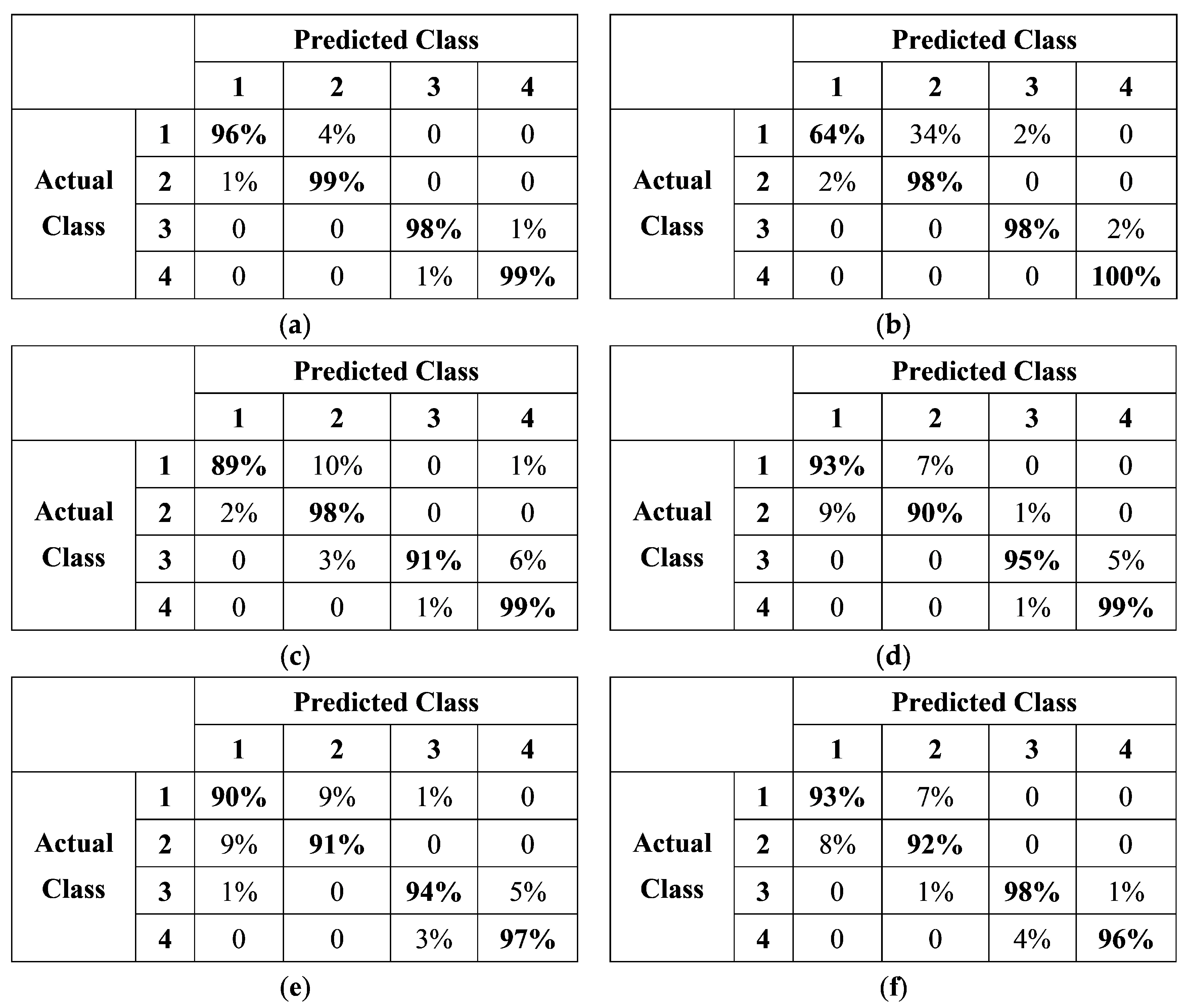
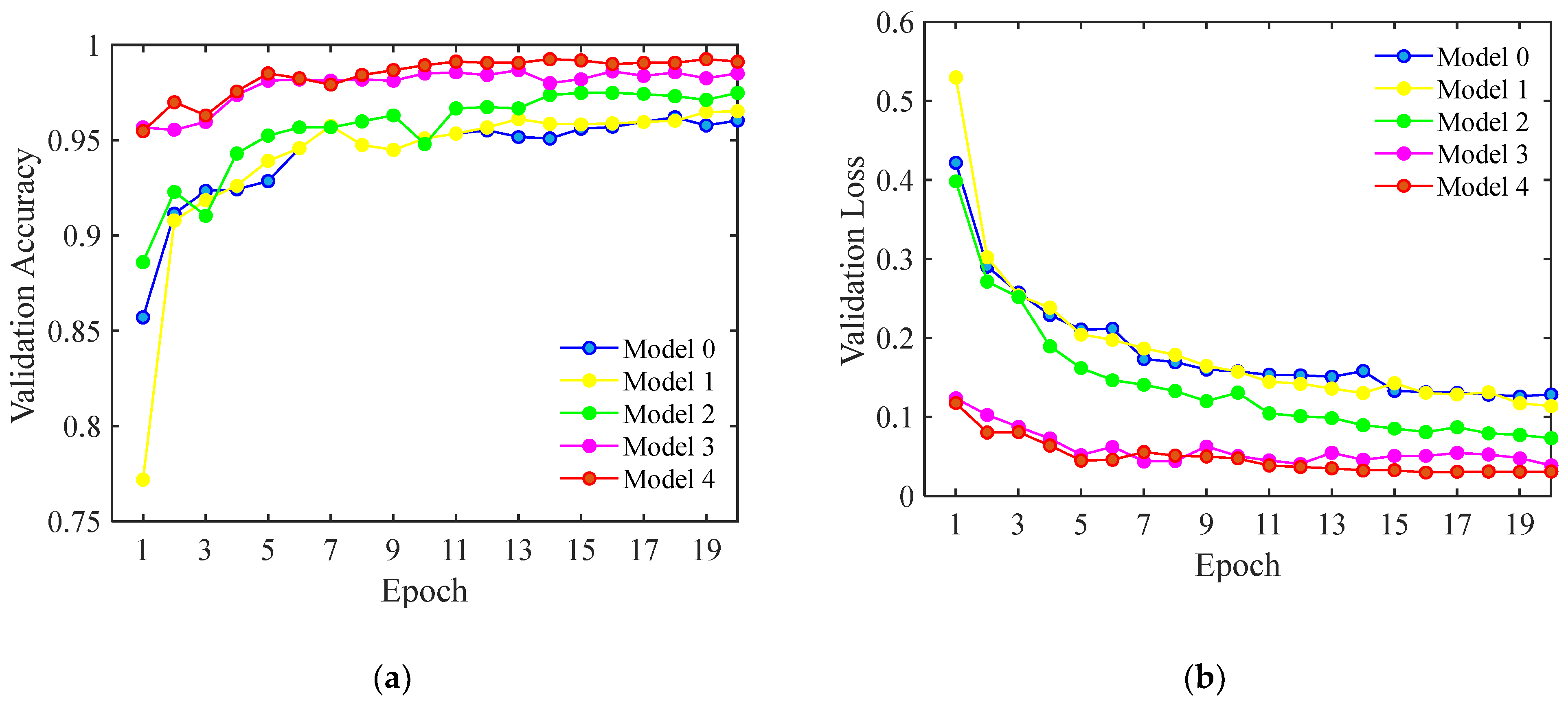
3.2.5. Performance Comparison after the Four Optimizations

To improve the quality grading performance of Oudemansiella raphanipes, the original MobileNetV2 model in Section 3.1 (Model 0), was continuously optimized by the data augmentation in Section 3.2.1 (Model 1), the hyperparameter selection in Section 3.2.2 (Model 2), the overfitting control strategy in Section 3.2.3 (Model 3), and the dynamic learning rate strategy in Section 3.2.4 (Model 4). In this section, the performances of these models are compared and discussed.

Figure 8 presents the validation accuracy and loss curves of the five models. With the increase in the optimization methods, the validation accuracy increases and the loss decreases. Moreover, their convergence speed is significantly accelerated. Taking Model 4 at the 20th epoch as an example, its validation accuracy and loss are 99.12% and 0.0295, respectively, showing a 3.35% increment and 0.1091 decrement, respectively, compared with those of Model 0 as shown in Figure 4.

Figure 9 gives the confusion matrixes of the four optimized models. Compared with the results of Model 0 shown in Figure 5d, the testing accuracies of all the four classes are improved. In particular, the problem of a low accuracy for distinguishing Class 1 from Class 2 in the original Model 0 is solved in the updated Model 4, in which the testing accuracies for Classes 1, 2, 3, and 4 are 98%, 99%, 98%, and 100%, respectively.

Table 3. The validation and testing performance of different models.

Model	Testing Accuracy (%)	Average Detection Time (ms)	Model Size (MB)	F1 Score (%)	Kappa Coefficient
Model 0	94.75	37.5	16.44	95.00	0.930
Model 1	96.25	45	16.44	96.30	0.948
Model 2	97.38	52.5	16.44	96.95	0.965
Model 3	98.00	23.75	16.48	98.00	0.973
Model 4	98.75	22.5	16.48	98.75	0.983

lists the testing accuracies, detection time for a single image, model size, F1 scores, and Kappa coefficients for the testing dataset. The F1 score, which takes into account both the precision and recall, can be calculated by Equation (1) [17,18,20].

$$\mathrm{F}1 \mathrm{Score}=2\times \frac{\mathrm{precision}\times \mathrm{recall}}{\mathrm{precision}+\mathrm{recall}},$$

(1)

where precision = TP/(TP + FP), recall = TP/(TP + FN), TP represents the quantity that the real value is 1 and the predicted value is 1, FP represents the quantity that the real value is 0 and the predicted value is 1, and FN represents the quantity that the real value is 1 and the predicted value is 0. The Kappa coefficient, which is a statistical indicator used for a consistency test; that is, whether the predicted results are consistent with the actual classification results, can be calculated by Equation (2) [19].

$$\mathrm{Kappa} \mathrm{coefficient}=\frac{{\mathrm{P}}_{\mathrm{o}}-{\mathrm{P}}_{\mathrm{e}}}{1-{\mathrm{P}}_{\mathrm{e}}},$$

(2)

where Po is the testing accuracy and Pe represents the sum of the actual number and predicted number of respective categories divided by the square of the total number of samples. It is shown that, with the increase in the optimization methods, all of the testing accuracies, F1 scores, and Kappa coefficients increase. Taking Model 4 as an example, its testing accuracy, F1 score, and Kappa coefficient are 98.75%, 98.75%, and 0.983, respectively, showing 4.00%, 3.75%, and 0.053 increments, respectively, compared with those of Model 0. The large F1 score and Kappa coefficient prove that the predicted results are almost perfectly consistent with the actual classification results. In addition, the detection time for a single image in Model 4 is 22.5 ms, which is 40% less than the 37.5 ms in Model 0, while the model size stays almost the same.

4. Discussion

The motivation of this work is for the quality grading of Oudemansiella raphanipes in a production line. The Oudemansiella raphanipes are placed on a carrier plate one by one and transported to an image-acquisition box, in which a color camera takes images of the Oudemansiella raphanipes and send the images to an industrial computer. The quality grading algorithm implements the classification and, then, the Oudemansiella raphanipes of different grades are grouped into different collection bins. As a result, the application of a quality grading algorithm requires not only a high accuracy but also a small detection time. Moreover, if cheaper computer resources are expected, a smaller model size is also required. On the premise of a relatively good accuracy, the basic MobileNetV2 model has the advantages of fast and efficient training, a small detection time, and small storage space compared with VGG16, ResNet50, InceptionV3, NasNet-Mobile, and EfficientNet. As a result, we selected MobileNetV2 as the basic model. Subsequently, the basic model was optimized by four strategies, including data augmentation, hyperparameter selecting, the overfitting control strategy, and the dynamic learning rate strategy; thereby, the convergence speed was accelerated and the classification accuracy was improved. The performance of the optimized MobileNetV2, of which the testing accuracy is 98.75%, the detection time for a single image is 22.5 ms, and the model size is 16.48 MB, satisfies the needs in the production line. Moreover, compared with the published papers on the classification of mushrooms using CNN [17,18,19,20], shown in

Table 4. Performance comparison between published papers and this paper.

Reference	Model	Testing Accuracy (%)	Detection Time (ms)	F1 Score (%)	Kappa Coefficient
[17]	6-layer CNN	74	/	74	/
[18]	InceptionV3	88.40	/	88	/
[19]	ResNet18	96.89	32	/	0.959
[20]	Modified AlexNet	98.5	/	99.09	/
This paper	Improved MobileNetV2	98.75	22.5	98.75	0.983

, our improved MobileNetV2 still has the highest testing accuracy, the lowest detection time, and the best consistency of the predicted results with the actual classification results.

Although the final classification accuracy can reach as high as 98.75%, the performance of the quality grading algorithm was only evaluated on the dataset of images with a simple background (see Figure 2). This simple background is applicable in a production line as described above. However, if the images are taken with a complex background, e.g., multiple Oudemansiella raphanipes in the soil, the classification accuracy would significantly decrease. The quality grading algorithm for Oudemansiella raphanipes in the soil is in progress and will be published in the near future.

5. Conclusions

To obtain a quality grading algorithm of Oudemansiella raphanipes by a deep CNN model, transfer leaning was adopted. Six typical CNN models, including VGG16, ResNet50, InceptionV3, NasNet-Mobile, EfficientNet, and MobileNetV2, were pretrained on the dataset of ImageNet and transferred to our dataset of Oudemansiella raphanipes. Considering both the testing accuracy and detection time, the MobileNetV2 was selected for further optimization. Four optimization methods, including data augmentation, hyperparameter selecting, the overfitting control strategy, and the dynamic learning rate strategy, were applied. As a result, the improved MobileNetV2 has advantages of a high efficiency, high speed, and small storage space. The testing accuracy is 98.75%, the detection time for a single image is 22.5 ms, and the model size is 16.48 MB. These characteristics are in line with the production practice.

References

1. Zhao, Y.; Wang, Y.; Li, K.; Mazurenko, I. Effect of Oudemansiella Raphanipes Powder on Physicochemical and Textural Properties, Water Distribution and Protein Conformation of Lower-Fat Pork Meat Batter. Foods 2022, 11, 2623. [Google Scholar] [CrossRef] [PubMed]
2. Azadnia, R.; Kheiralipour, K. Recognition of Leaves of Different Medicinal Plant Species Using a Robust Image Processing Algorithm and Artificial Neural Networks Classifier. J. Appl. Res. Med. Aromat. Plants 2021, 25, 100327. [Google Scholar] [CrossRef]
3. Seydi, S.T.; Amani, M.; Ghorbanian, A. A Dual Attention Convolutional Neural Network for Crop Classification Using Time-series Sentinel-2 Imagery. Remote Sens. 2022, 14, 498. [Google Scholar] [CrossRef]
4. Moreno-Revelo, M.Y.; Guachi-Guachi, L.; Gómez-Mendoza, J.B.; Revelo-Fuelagán, J.; Peluffo-Ordóñez, D.H. Enhanced Convolutional-Neural-Network Architecture for Crop Classification. Appl. Sci. 2021, 11, 4292. [Google Scholar] [CrossRef]
5. Yu, Q.; Yang, H.; Gao, Y.; Ma, X.; Chen, G.; Wang, X. LFPNet: Lightweight Network on Real Point Sets for Fruit Classification and Segmentation. Comput. Electron. Agric. 2022, 194, 106691. [Google Scholar] [CrossRef]
6. Ghazal, S.; Qureshi, W.S.; Khan, U.S.; Iqbal, J.; Rashid, N.; Tiwana, M.I. Analysis of Visual Features and Classifiers for Fruit Classification Problem. Comput. Electron. Agric. 2021, 187, 106267. [Google Scholar] [CrossRef]
7. Hossain, M.S.; Al-Hammad, M.; Muhammad, G. Automatic Fruit Classification Using Deep Learning for Industrial Applications. IEEE Trans. Industr. Inform. 2018, 15, 1027–1034. [Google Scholar] [CrossRef]
8. Altaheri, H.; Alsulaiman, M.; Muhammad, G. Date Fruit Classification for Robotic Harvesting in a Natural Environment Using Deep Learning. IEEE Access 2019, 7, 117115–117133. [Google Scholar] [CrossRef]
9. Ahmed, M.I.; Mamun, S.M.; Asif, A.U.Z. DCNN-Based Vegetable Image Classification Using Transfer Learning: A Comparative Study. In Proceedings of the 5th International Conference on Computer, Communication and Signal Processing (ICCCSP), Chennai, India, 24–25 May 2021. [Google Scholar]
10. Ulloa, C.C.; Krus, A.; Barrientos, A.; Del Cerro, J.; Valero, C. Robotic Fertilization in Strip Cropping Using a CNN Vegetables Detection-Characterization Method. Comput. Electron. Agric. 2022, 193, 106684. [Google Scholar] [CrossRef]
11. Hameed, K.; Chai, D.; Rassau, A. A Comprehensive Review of Fruit and Vegetable Classification Techniques. Image Vis. Comput. 2018, 80, 24–44. [Google Scholar] [CrossRef]
12. Sujatha, R.; Chatterjee, J.M.; Jhanjhi, N.Z.; Brohi, S.N. Performance of Deep Learning vs Machine Learning in Plant Leaf Disease Detection. Microprocess. Microsyst. 2021, 80, 103615. [Google Scholar] [CrossRef]
13. Esgario, J.G.M.; Krohling, R.A.; Ventura, J.A. Deep Learning for Classification and Severity Estimation of Coffee Leaf Biotic Stress. Comput. Electron. Agric. 2020, 169, 105162. [Google Scholar] [CrossRef] [Green Version]
14. Arwatchananukul, S.; Kirimasthong, K.; Aunsri, N. A New Paphiopedilum Orchid Database and Its Recognition Using Convolutional Neural Network. Wireless. Pers. Commun. 2020, 115, 3275–3289. [Google Scholar] [CrossRef]
15. Ji, M.; Zhang, K.; Wu, Q.; Deng, Z. Multi-label Learning for Crop Leaf Diseases Recognition and Severity Estimation Based on Convolutional Neural Networks. Soft Comput. 2020, 24, 15327–15340. [Google Scholar] [CrossRef]
16. Suharjito Elwirehardja, G.N.; Prayoga, J.S. Oil Palm Fresh Fruit Bunch Ripeness Classification on Mobile Devices Using Deep Learning Approaches. Comput. Electron. Agr. 2021, 188, 106359. [Google Scholar] [CrossRef]
17. Preechasuk, J.; Chaowalit, O.; Pensiri, F.; Visutsak, P. Image Analysis of Mushroom Types Classification by Convolution Neural Networks. In Proceedings of the 2nd Artificial Intelligence and Cloud Computing Conference (AICCC), Kobe, Japan, 21–23 December 2019. [Google Scholar]
18. Zahan, N.; Hasan, M.Z.; Malek, M.A.; Reya, S.S. A Deep Learning-Based Approach for Edible, Inedible and Poisonous Mushroom Classification. In Proceedings of the International Conference on Information and Communication Technology for Sustainable Development (ICICT4SD), Dhaka, Bangladesh, 27–28 February 2021. [Google Scholar]
19. Zhao, M.; Li, Y.; Xu, P.; Song, T.; Li, H. Image Classification Method for Oudemansiella Raphanipes Using Compound Knowledge Distillation Algorithm. Trans. Chin. Soc. Agric. Eng. 2021, 37, 303–309. [Google Scholar]
20. Ketwongsa, W.; Boonlue, S.; Kokaew, U. A New Deep Learning Model for the Classification of Poisonous and Edible Mushrooms Based on Improved AlexNet Convolutional Neural Network. Appl. Sci. 2022, 12, 3409. [Google Scholar] [CrossRef]
21. Sandler, M.; Howard, A.; Zhu, M.; Zhmoginov, A.; Chen, L.C. Mobilenetv2: Inverted Residuals and Linear Bottlenecks. In Proceedings of the 2018 IEEE Conference on Computer Vision and Pattern Recognition (CVPR), Salt Lake City, UT, USA, 18–23 June 2018. [Google Scholar]
22. Srinivasu, P.N.; SivaSai, J.G.; Ijaz, M.F.; Bhoi, A.K.; Kim, W.; Kang, J.J. Classification of Skin Disease Using Deep Learning Neural Networks with MobileNetV2 and LSTM. Sensors 2021, 21, 2852. [Google Scholar] [CrossRef]
23. Lin, Z.; Guo, W. Cotton Stand Counting from Unmanned Aerial System Imagery Using MobileNet and CenterNet Deep Learning Models. Remote Sens. 2021, 13, 2822. [Google Scholar] [CrossRef]
24. Kim, M.; Kwon, Y.; Kim, J.; Kim, Y. Image Classification of Parcel Boxes Under the Underground Logistics System Using CNN MobileNet. Appl. Sci. 2022, 12, 3337. [Google Scholar] [CrossRef]
25. Sun, H.; Zhang, S.; Ren, R.; Su, L. Maturity Classification of “Hupingzao” Jujubes with an Imbalanced Dataset Based on Improved MobileNetV2. Agriculture 2022, 12, 1305. [Google Scholar] [CrossRef]
26. Li, Y.; Xue, J.; Wang, K.; Zhang, M.; Li, Z. Surface Defect Detection of Fresh-Cut Cauliflowers Based on Convolutional Neural Network with Transfer Learning. Foods 2022, 11, 2915. [Google Scholar] [CrossRef] [PubMed]
27. Simonyan, K.; Zisserman, A. Very Deep Convolutional Networks for Large-Scale Image Recognition. In Proceedings of the 2015 International Conference on Learning Representations (ICLR), San Diego, CA, USA, 7–9 May 2015. [Google Scholar]
28. He, K.; Zhang, X.; Ren, S.; Sun, J. Deep Residual Learning for Image Recognition. In Proceedings of the 2016 IEEE Conference on Computer Vision and Pattern Recognition (CVPR), Las Vegas, NV, USA, 27–30 June 2016. [Google Scholar]
29. Szegedy, C.; Vanhoucke, V.; Ioffe, S.; Shlens, J.; Wojna, Z. Rethinking the Inception Architecture for Computer Vision. In Proceedings of the 2016 IEEE Conference on Computer Vision and Pattern Recognition (CVPR), Las Vegas, NV, USA, 27–30 June 2016. [Google Scholar]
30. Zoph, B.; Vasudevan, V.; Shlens, J.; Le, Q.V. Learning Transferable Architectures for Scalable Image Recognition. In Proceedings of the 2018 IEEE Conference on Computer Vision and Pattern Recognition (CVPR), Salt Lake City, UT, USA, 18–23 June 2018. [Google Scholar]
31. Tan, M.; Le, Q. Efficientnet: Rethinking Model Scaling for Convolutional Neural Networks. In Proceedings of the 2019 International Conference on Machine Learning (ICML), Long Beach, CA, USA, 9–15 June 2019. [Google Scholar]
32. Mehta, S.; Rastegari, M. MobileViT: Light-Weight, General-Purpose, and Mobile-Friendly Vision Transformer. arXiv 2021, arXiv:2110.02178. [Google Scholar]
33. Kogilavani, S.V.; Prabhu, J.; Sandhiya, R.; Kumar, M.S.; Subramaniam, U.; Karthick, A.; Imam, S.B.S. COVID-19 Detection Based on Lung CT Scan Using Deep Learning Techniques. Comput. Math. Methods Med. 2022, 2022, 7672196. [Google Scholar] [CrossRef]
34. Deng, J.; Dong, W.; Socher, R.; Li, L.J.; Li, K.; Fei-Fei, L. Imagenet: A Large-Scale Hierarchical Image Database. In Proceedings of the 2009 IEEE Conference on Computer Vision and Pattern Recognition (CVPR), Miami, FL, USA, 20–25 June 2009. [Google Scholar]
35. Ioffe, S.; Szegedy, C. Batch normalization: Accelerating Deep Network Training by Reducing Internal Covariate Shift. In Proceedings of the 32nd International Conference on Machine Learning (ICML 2015), Lille, France, 6–11 July 2015. [Google Scholar]
36. Srivastava, N.; Hinton, G.; Krizhevsky, A.; Sutskever, I.; Salakhutdinov, R. Dropout: A Simple Way to Prevent Neural Networks from Overfitting. J. Mach. Learn. Res. 2014, 15, 1929–1958. [Google Scholar]
Figure 1. Experimental setup for image acquisition.
Horticulturae 08 01119 g001
Figure 2. Four quality levels of Oudemansiella raphanipes. (a) Class 1; (b) Class 2; (c) Class 3; (d) Class 4.
Horticulturae 08 01119 g002
Figure 3. Transfer leaning method for MobileNetV2.
Horticulturae 08 01119 g003
Figure 4. The validation (a) accuracies and (b) losses of VGG16, ResNet50, InceptionV3, NasNet-Mobile, EfficientNetB0, and MobileNetV2.
Horticulturae 08 01119 g004
Figure 5. The confusion matrixes of (a) VGG16, (b) ResNet50, (c) InceptionV3, (d) NasNet-Mobile, (e) EfficientNetB0, and (f) MobileNetV2 applied on testing dataset.
Horticulturae 08 01119 g005
Figure 6. The validation (a) accuracies and (b) losses of the cases with different overfitting control strategies.
Horticulturae 08 01119 g006
Figure 7. The validation (a) accuracies and (b) losses of the cases with different learning rates.
Horticulturae 08 01119 g007
Figure 8. The validation (a) accuracies and (b) losses of different models.
Horticulturae 08 01119 g008
Figure 9. The confusion matrixes of (a) Model 1, (b) Model 2, (c) Model 3, and (d) Model 4.
Horticulturae 08 01119 g009