Article

Effect of Stand Reduction at Different Growth Stages on Yield of Paprika-Type Chile Pepper

Extension Plant Sciences, New Mexico State University, P.O. Box 30003, MSC 3AE, Las Cruces, NM 88003, USA
*
Author to whom correspondence should be addressed.
Horticulturae 2020, 6(1), 16; https://doi.org/10.3390/horticulturae6010016
Submission received: 16 December 2019 / Revised: 30 January 2020 / Accepted: 24 February 2020 / Published: 5 March 2020

Abstract

:
Paprika-type chile (Capsicum annuum L.) crops are susceptible to plant population losses through pest activity, disease, and extreme weather events such as hail storms. This study was conducted to determine the influence of intensity and timing of plant population reductions on the final harvested yield of paprika-type chile so that informed decisions can be made regarding continuing or ending a damaged field. Two trials, one per year, were conducted in southern New Mexico. ‘LB-25’, a standard commercial cultivar, was direct seeded on 29 March 2016 and 4 April 2017. Plants were thinned at three different growth stages; early seedling, first bloom, and peak bloom. Plants were thinned to four levels at each phenological stage; 0% stand reduction (control; ~200,000 plants/ha), 60% stand reduction (~82,000 plants/ha), 70% stand reduction (~60,000 plants/ha), and 80% stand reduction (~41,000 plant/ha). In both years, the main effects of stand reduction had a significant impact on harvested yield, emphasizing the percentage of stand reduction has more of an impact on yield than timing in paprika-type red chile. Consistently, an 80% stand reduction in paprika-type chile significantly reduced fresh red chile yield by 26% to 38%.

1. Introduction

Crop hail damage can cause considerable economic loss during the growing season [1]. Physical crop injury can be divided into two main categories; defoliation and stand reduction [2]. Many researchers have simulated stand reduction in crops such as cotton (Gossypium hirsutum L.), corn (Zea mays L.), soybeans (Glycine max L.), and wheat (Triticum aestivum L.) by cutting and removing a specific number of plants from the field [2,3,4]. Conversely, for many vegetable crops including paprika-type chile, little to no research of a similar type has been conducted [1].
Paprika-type red chile (Capsicum annuum L.) is a specialty crop important in the southwest region of the United States with a total of 5382 ha of red chile harvested in New Mexico, Arizona, and Texas in 2016 [5,6]. Stand reductions due to pests and extreme weather events have been identified as threats to chile farmers in both Arizona and New Mexico. In response to these threats, the United States Department of Agriculture Risk Management Agency has started pilot programs to insure chile crops [7]. For example, in 2016, there were 136 hail events in New Mexico, 29 hail events in Arizona, and over 500 hail events in Texas [8], causing both defoliation and stand reduction damage to crops. To adequately insure and provide coverage for losses in chile, both farmers and insurance companies must have information on how chile yield changes due to stand reduction caused by pests or extreme weather events at different growth stages.
In the southwest US, New Mexico-type green and red chile are the two most prominent chile products. New Mexico-type red chile is harvested when fruit are at a mature red stage and are partially dried on the plant [9]. Paprika-type chile is a subset of red chile distinctive for fruit exhibiting very low heat level and high carotenoid content [10]. Carotenoids are extracted and used as a natural dye in a variety of food and cosmetic products [11]. Paprika-type chile is also ground into powder and used as a spice [12]. New Mexico is the only state in the southwest to categorize chile production, and in 2016, the highest harvested category of chile was paprika-type chile at 1416 ha [13]. Paprika-type chile was selected for this study due to its importance, not only in the southwest, but to the food industry all over the world. Throughout the world, red paprika-type chile is used as a culinary spice and the extracted pigments of paprika-type red chile are used a natural food colorant in many food products.
All of the previously reported research on the effect of plant population losses in paprika-type chile has been done at one growth stage, leaving a gap in the knowledge about responses during different growth stages. As Cavero et al. [14] found, paprika yield increased as plant density increased from 13,333 to 200,000 plants per hectare when the plants were thinned during the ten to twelve leaves growth stage. Although this illustrated that there is an impact on paprika-type red chile when plant populations change, how they respond to such changes over the season has not been explored. On the other hand, a paprika-type chile field with a high plant population density of 322,335 plants per hectare experienced a 60% yield reduction [10]. It has been reported that removing plants from fields with high plant populations at specific growth stages can be beneficial due to reduction in competition for light [15]. Pariossien and Flynn [10] reported the best planting density for paprika-type red chile to be 98,800 plants per hectare.
In other crops such as soybeans, when plant populations were reduced at the early growth stage, there were no significant changes in seed yield, but when stand reduction occurred in the later growth stage seed yield was decreased [2]. Similar results were found when sunflowers (Helianthus annuus L.) underwent stand reduction at early and late growth stages. Sunflower stand losses of 25% during later growth stages significantly reduced yield, while no reductions in yield occurred when stand losses of 25% occurred at an early growth stage [16]. Many crops can compensate for stand reduction losses early in the season.
The goal of this study was to understand how a simulation of population losses by stand reduction at different growth stages affected the yield of paprika-type red chile. Obtaining this knowledge will give farmers more insight into their yield expectations after a stand reduction event caused by pests and/or extreme weather events at any growth stage. The specific objectives were to determine how four levels of stand reduction simulating hail damage at three growth stages affect the yield components. Our hypothesis was that paprika-type red chile, an indeterminate crop, would recover from stand reduction early in the growing season.

2. Materials and Methods

Field experiments were conducted during 2016 and 2017 at the New Mexico State University Leyendecker Plant Science Research Center in La Mesa, NM, USA [ LPSRC (lat. 32.16° N; long. 106.46° W; elevation 1186 m)]. The soil at LPSRC was a Glendale clay loam [17]. Fertilization during both years consisted of total nitrogen (Helena Chemicals, Collierville, TN, USA) at 168.1 kg·ha−1 and total phosphorus at 112.1 kg·ha−1. All phosphorus and a quarter of the nitrogen were broadcast preplant as ammonium phosphate and the remaining nitrogen was delivered throughout the season in the irrigation water as urea and ammonium nitrate.

2.1. Field Cultivation

The field was plowed, disced, laser-leveled, and listed before planting. ‘LB-25’ (Biad Chili Co., Leasburg, NM, USA), a common commercial paprika-type red chile cultivar, was planted at a rate of 5.6 kg·ha−1 on 29 March 2016 and 4 April 2017 with metalaxyl fungicide (Ridomil Gold; Syngenta, Greensboro, NC, USA) at 146 mL·ha−1 banded into the planting bed during the direct seeding of the ‘LB-25’. A two-way factorial treatment structure in a randomized complete block design with four replications for a total of 48 plots was used. The first factor, stand reduction, had four levels, and the second factor, growth stage, had three levels, and each were combined and randomized in the field plot. Each plot consisted of three rows, with a total area of 13.8 m2 (3.0 m between row spacing × 4.6 m length). The field was 662.24 m2 (13.8 m2 × 48 plots) surrounded by one row (north and south) or plot (east and west) borders of paprika-type red chile plants. All plots were hand-weeded weekly each season. The field was furrow irrigated once every 10–14 days and irrigation ended on 16 September 2016 and 1 September 2017 when the crop was at a mature red growth stage.

2.2. Stand Reduction

At three different growth stages, plants were thinned to four levels of stand reduction. When plants were thinned, two plants were left in a clump [18] at different spacing intervals to achieve desired plant counts per plot. When describing stand reduction treatments, a row is one of the three rows within a plot with an area of 4.6 m2 (1.0 m × 4.6 m). Each of the three rows in a plot were thinned to one of the specified treatments. The four stand reductions treatments were: control with no thinning and ~64 plants per row, 60% stand reduction with 35.7-cm spacing and ~25 plants per row, 70% stand reduction with 45.7-cm spacing and ~19 plants per row, and 80% stand reduction with 66.0-cm spacing and ~13 plants per row. The densities achieved in 2016 for each stand reduction level were 209,974 plants·ha−1 (control, no thinning), 82,021 plants·ha−1 (60% stand reduction), 62,336 plants·ha−1 (70% stand reduction), and 42,651 plants·ha−1 (80% stand reduction). The densities achieved in 2017 for each stand reduction level were 200,131 plants·ha−1 (control, no thinning), 82,021 plants·ha−1 (60% stand reduction), 59,055 plants·ha−1 (70% stand reduction), and 39,370 plants·ha−1 (80% stand reduction).

2.3. Growth Stages

Stand reduction treatments occurred at pre-determined growth stages based on heat units accumulated after planting (HUAP). HUAP values were calculated using the method described by Brown [19] and Silvertooth et al. [20] (Table 1 and Table 2) using 12 °C as the base temperature. Using heat unit systems in a phenology model for crops relates plant growth to local weather and climate conditions [19] and take into account day to day changes in temperature [20]. Daily weather data such as maximum temperatures, minimum temperatures, mean temperatures, and precipitation were collected from the LPSRC weather station, La Mesa, NM, USA [21,22] (Table 1 and Table 2).
The targeted growth stages for the stand reduction treatments were early seedling stage at 700 HUAP, first bloom at 1400 HUAP, and peak bloom at 2000 HUAP [20]. Although HUAP values were used to determine phenological growth stages, we observed that early seedling stage was characterized by the plants having about 30 true leaves, 60–70 days after planting. First bloom was when anthesis began on each plant and peak bloom when more than 60% anthesis was observed. Due to inclement weather and scheduling constraints, stand reduction events did not occur at the exact targeted number of HUAPs for each growth stage. The actual HUAPs and dates for each stand reduction event in 2016 were: early seedling stage on 1 June 2016 at 623 HUAP, first bloom on 27 June 2016 at 1268 HUAP, and peak bloom on 19 July 2016 at 1849 HUAP. The actual HUAPs and dates for each stand reduction event in 2017 were: early seedling stage on 31 May 2017 at 717 HUAP, first bloom on 26 June 2017 at 1398 HUAP, and peak bloom on 17 July 2017 at 1894 HUAP.

2.4. Harvest

The plots were harvested on 17 October 2016 at 3598 HUAP and on 25 October 2017 at 3629 HUAP. The harvested sample area was 3.1 m2 (3.04 m × 1.01 m) taken from the middle section of the middle row of each plot. In 2017, due to labor constraints, the sample size was reduced to 1.5 m2 (1.52 m × 1.01 m). All fruit within a sample area was hand-harvested into plastic bags and then removed from the field for sorting.

2.5. Yield Data Collection

Harvested material was sorted into the following categories: (1) fresh red yield, (2) fresh green yield, (3) unmarketable yield, (4) immature yield. Fruit classified as red were fruits with more than 50% red color. Fruit classified as green were fruits with more than 50% green color. Fruit classified as unmarketable yield were fruits with blemishes and/or discoloration from disease covering over 40% of the fruit. Immature fruit were fruits under 7.6-cm and had a malleable pericarp. Immature yield was nominal, so data were not included in this report. All of the sorted material was weighed (SVI-100E; Sartorius Stedim North America, Bohemia, NY, USA). Fresh red yield was put in a drier at 54.4 °C until fruit were completely dehydrated and then weighed for a dry red yield. In 2016, red yield subsamples in the drier were overcome with mold and had to be discarded.

2.6. Data Analysis

Additionally, this study was designed to measure and compare the interaction of stand reduction and growth stage on various yield components. Analysis was conducted on each year separately due to environmental variation between the years. Response variables analyzed in 2016 and 2017 were: fresh red yield, green yield, unmarketable yield, and plant counts. Additionally, dry red yield was analyzed in 2017, but not in 2016 due to the mold growth noted above. Response variable data were analyzed by analysis of variance (ANOVA) using SAS (version 9.4; SAS Institute, Cary, NC, USA). Tukey’s significant difference test (p ≤ 0.05) was used to separate means when interactions between stand reduction level and growth stage were significant. When interactions were not significant, ANOVA was conducted on the main effects of stand reduction levels. If statistically significant differences were detected in the main effects, then Tukey’s significant difference test (p ≤ 0.05) was used to separate means.

3. Results

3.1. Weather Differences

There were two major differences in weather patterns between the 2016 and 2017 growing seasons. First, 2017 had an overall higher average minimum temperature for the entire season. In 2016, the season average minimum temperature was 13.7 °C, 0.5 °C cooler than in 2017. The higher minimum temperatures 2017 increased the growth rate of the plants, so they matured at a faster rate. Due to this, the 2017 season was 28 weeks long and the 2016 season was 30 weeks long. Second, 2017 had 5.2 cm more total precipitation during the growing season. Much of the precipitation recorded in 2017 occurred in the month of July 2017; it fell at a fast rate, leaving the field with standing water for over a week from 17 July through 24 July 2017.

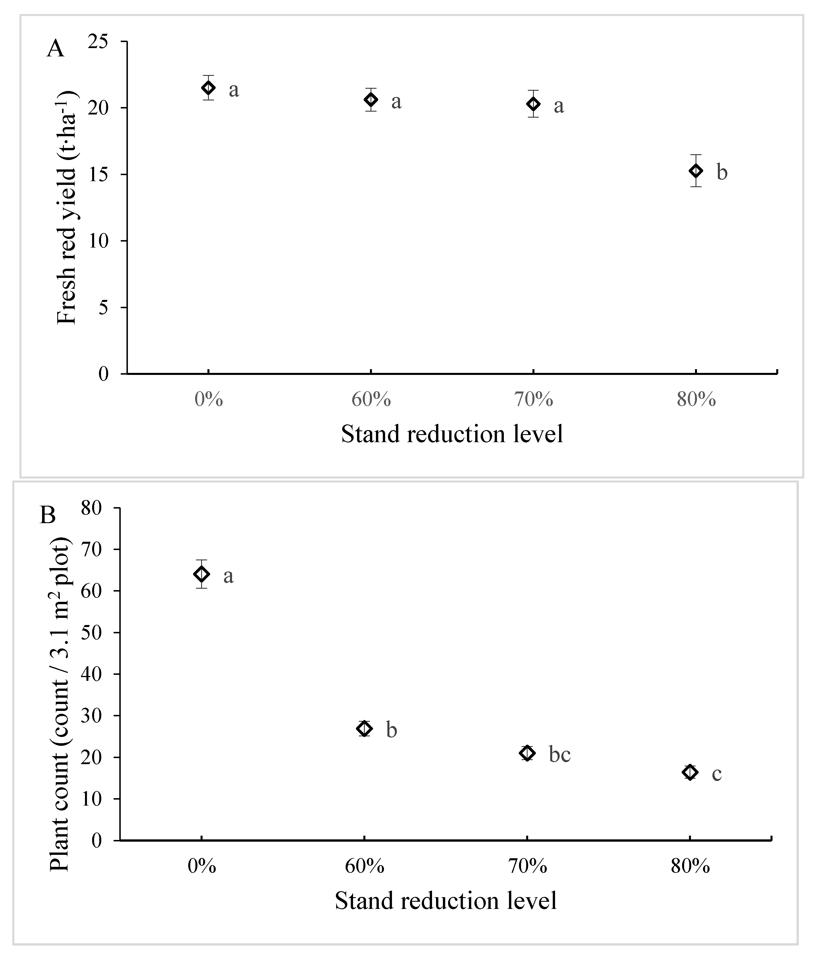
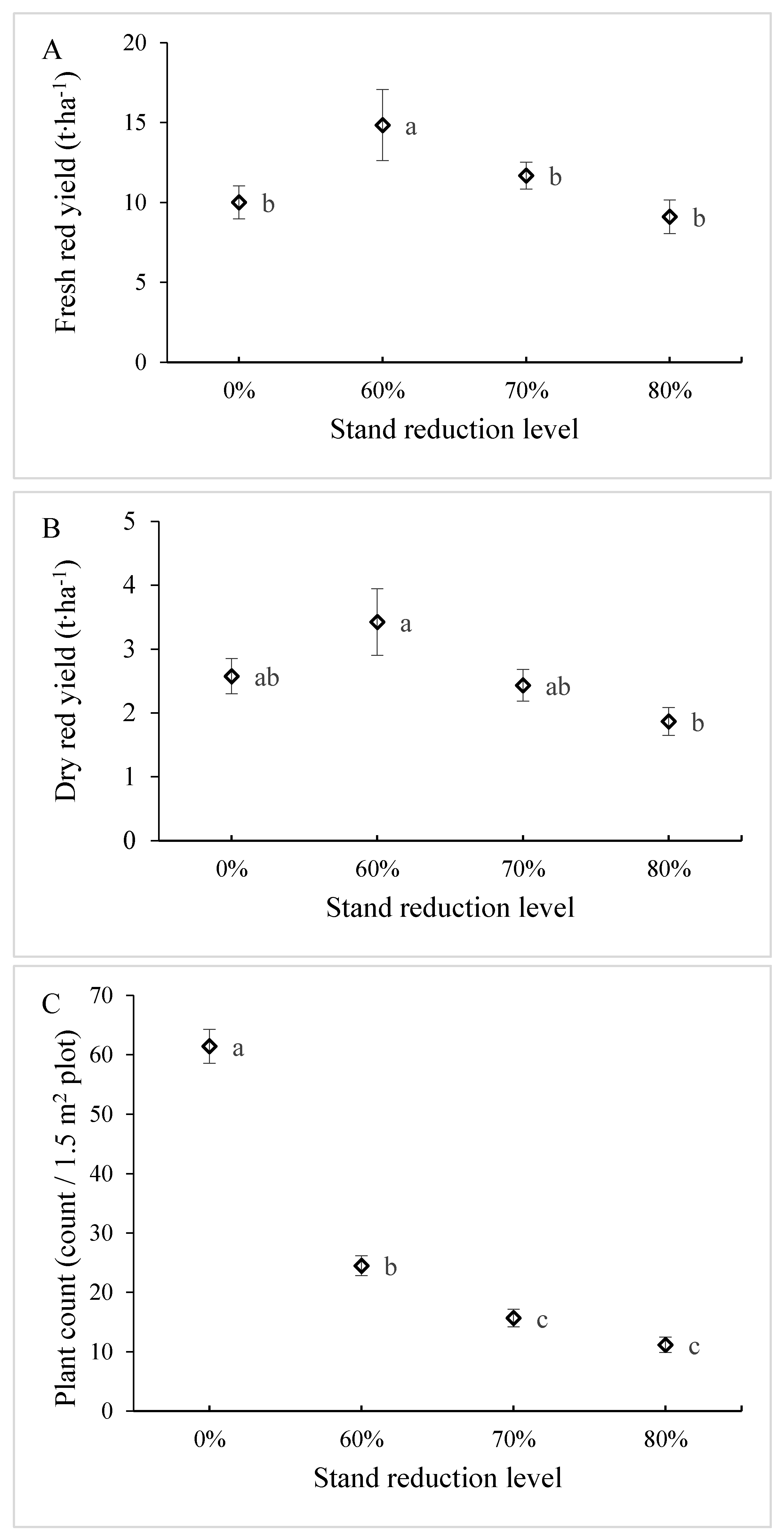
3.2. Yield Components

Growth stage by stand reduction interactions were not statistically significant for all of the yield components measured in 2016 and 2017 (Table 3 and Table 4). So significant stand reduction main effects were evaluated. In 2016, stand reduction had a significant impact on fresh red fruit yield and plant counts (Table 3). The 0%, 60%, and 70% stand reduction plots had on average 36% more fresh red fruit yield than the 80% stand reduction plots (Figure 1A). As expected, the 0% stand reduction plots had over two and a half times more plants than the 80% and 70% stand reduction plots (Figure 1B). In 2017, stand reduction had an effect on fresh red fruit yield, dry red fruit yield, and plant counts (Table 4). The 60% stand reduction plots in 2017 had 45% more fresh red yield than the 0%, 70%, and 80% stand reduction plots (Figure 2A). The 60% stand reduction plots also had 83% more dry red yield than the 80% stand reduction plots (Figure 2B). When evaluating the plant counts, the 0% stand reduction plots had over four times the number of plants as the 80% stand reduction plots (Figure 2C).

4. Discussion

We found that the timing of stand reductions for paprika-type chile did not impact marketable red yields at the end of the season. Studies conducted in soybeans and sunflowers showed that yield was significantly impacted by the growth stage during which a stand reduction occurs. When sunflower plant populations were reduced in early growth stages they were able to recover yield, but stand losses in later growth stages resulted in yield reductions [16]. Similar results were found in soybeans when stand losses occurred in the early growth stages and yield was not affected due to plant compensation [2]. Yet, we found paprika-type chile yield was not affected by the growth stage during which stand reduction occurred. This could be due to our methodology of thinning the plots to clumps of 2 to 3 plants [18]. This standard practice, long employed by red chile growers in New Mexico, may provide protection from yield losses by increasing interplant competition. Interplant competition driven by clumped plants may increase vigorous plant growth earlier in the season [9] producing robust plants by midseason that are able to compensate for plants lost. Additionally, we may not have decreased plant populations at optimal growth stages to have an impact on yield components. Our 70% and 80% stand reduction plots did not have statistically different plant counts in either 2016 or 2017; perhaps a 90% stand reduction plot was necessary.
In 2017, our control plots with 0% stand reduction had less fresh and dry red yields. Reports have shown that chile grown in dense populations will yield less due to a decrease in plant light reception [10,23]. Our lower yields in 2017 may suggest that some thinning might be necessary to ensure each plant has access to light and enough space to adequately grow.
Traditionally, when evaluating how crops respond to stand reductions due to pest and/or extreme weather damage, two variables are taken into consideration: growth stage and extent of crop loss [16,24,25]. Our yield components were not significantly affected by the growth stage during the stand reduction event. The percentage of stand losses had a greater impact on the fresh red yield and dry red yield of paprika-type chile. According to our results, percentage of crop loss is a better predictor of end of season crop loss than the growth stage during which the stand reduction occurs. Therefore, insurance adjusters and farmers can estimate paprika-type chile crop losses based on percentage of stand losses instead of growth stage. Fresh red yield will be significantly reduced by 26% to 38% when plant populations are reduced by 80%. Cavero et al. [14] had comparable yield loss results, indicating paprika-type chile has some capacity to recover and compensate for stand reduction losses. This has been observed in other indeterminate crops such as lentils (Lens culinaris L.) that can compensate for stand reduction caused by hail damage anytime during the season [26]. Our data shows that a farmer could lose up to 70% of their paprika-type chile stand (a remaining plant population of at least 60,000 plants per hectare) due to hail damage and experience minimal to no impact on their yields.

Author Contributions

I.J., conception or design of the work, and the acquisition, analysis, or interpretation of data for the work, wrote initial draft of manuscript, and completed edits. S.W., conception or design of the work, co-authored initial draft of manuscript, and completed edits. All authors have read and agreed to the published version of the manuscript.

Funding

This research received no additional funding.

Conflicts of Interest

The authors declare no conflict of interest.

References

  1. Sij, J.W.; Ott, J.P.; Olson, B.L.; Baughman, T.A. Growth and yield response to simulated hail damage in guar. Agron. J. 2005, 97, 1636–1639. [Google Scholar] [CrossRef] [Green Version]
  2. Teigen, J.B.; Vorst, J.J. Soybean response to sand reduction and defoliation. Agron. J. 1975, 67, 813–816. [Google Scholar] [CrossRef]
  3. McGinty, J.; Morgan, G.; Mott, D. Cotton response to simulated hail damage and stand loss in central Texas. J. Cotton Sci. 2019, 23, 1–6. [Google Scholar]
  4. Vorst, J.V. Assessing hail damage to corn. In National Corn Handbook; Iowa State University: Ames, IA, USA, 1990; Volume 1, p. 4. [Google Scholar]
  5. Soto-Ortiz, R.; Silvertooth, J.C.; Galadima, A. Crop Phenology for Irrigated Chiles (Capsicum Annuum L.) in Arizona and New Mexico; University of Arizona Vegetable Report; University of Arizona: Tucson, AZ, USA, 2006. [Google Scholar]
  6. United States Department of Agriculture. Vegetables: 2016 Summary. 2017. Available online: http://usda.mannlib.cornell.edu/usda/current/VegeSumm/VegeSumm-02-22-2017_revision.pdf (accessed on 2 January 2018).
  7. United States Department of Agriculture. Risk Management Agency State Profiles. 2017. Available online: https://www.rma.usda.gov/pubs/state-profiles.html (accessed on 3 January 2018).
  8. National Oceanic and Atmospheric Administration. Storm Event Database. 2016. Available online: https://www.ncdc.noaa.gov/stormevents/ (accessed on 3 January 2018).
  9. Walker, S.J.; Funk, P.A. Mechanizing chile peppers: Challenges and advances in transitioning harvest of New Mexico’s signature crop. HortTechnology 2014, 3, 281–284. [Google Scholar] [CrossRef]
  10. Paroissien, M.; Flynn, R. Plant spacing/plant population for machine harvest. In New Mexico Chile Task Force. Rpt 13; New Mexico State Univeristy: Las Cruces, NM, USA, 2004. [Google Scholar]
  11. Wolf, I.; Aper, Y. Mechanization of paprika harvest. In Proceedings of the First International Conference on Fruit, Nut and Vegetable Harvesting Mechanization, Bet Dagan, Israel, 5–12 October 1983; American Society of Agricultural and Biological Engineers: St. Joesph, MI, USA, 1984; Volume 5, pp. 265–275. [Google Scholar]
  12. Bosland, P.W.; Votava, E.J. Pepper: Vegetable and Spice Capsicums; CABI Publishers: Oxon, UK, 2000. [Google Scholar]
  13. New Mexico Department of Agriculture. 2016 New Mexico Chile Production. 2016. Available online: https://www.nass.usda.gov/Statistics_by_State/New_Mexico/Publications/Special_Interest_Reports/NM_Chile_Production_03012017.pdf (accessed on 2 January 2018).
  14. Cavero, J.; Ortega, R.G.; Guitierrez, M. Plant density affects yield, yield components, and color of direct-seeded paprika pepper. HortScience 2001, 36, 76–79. [Google Scholar] [CrossRef]
  15. Donald, C.M. Competition among crop and pasture plants. Adv. Agron. 1963, 15, 1–118. [Google Scholar]
  16. Miller, J.F.; Roath, W.W. Compensatory response of sunflower to stand reduction applied at different plant growth stages. Agron. J. 1982, 74, 119–121. [Google Scholar] [CrossRef]
  17. Natural Resources Conservation Service. Web Soil Survey. 2017. Available online: https://websoilsurvey.sc.egov.usda.gov/App/WebSoilSurvey.aspx (accessed on 20 October 2017).
  18. Bosland, P.W.; Walker, S.J. Growing chiles in New Mexico. In New Mexico State Cooperative Extension Services Guide H-230; Mew Mexico State University: Las Cruces, NM, USA, 2004. [Google Scholar]
  19. Brown, P.W. Heat Units. University of Arizona Cooperative Extension Bulletin AZ1602; University of Arizona: Tucson, AZ, USA, 2012. [Google Scholar]
  20. Silvertooth, J.C.; Brown, P.W.; Walker, S.J. Crop growth and development for irrigated chile (Capsicum annuum). In New Mexico Chile Task Force Report 32; New Mexico State University: Las Cruces, NM, USA, 2010. [Google Scholar]
  21. New Mexico Climate Center. Leyendecker II PSRC Weather Data. 2016. Available online: https://weather.nmsu.edu/ziamet/request/station/nmcc-da-5/data/ (accessed on 5 January 2018).
  22. New Mexico Climate Center. Leyendecker II PSRC Weather Data. 2017. Available online: https://weather.nmsu.edu/ziamet/request/station/nmcc-da-5/data/ (accessed on 5 January 2018).
  23. Decoteau, D.R.; Graham, H.A.H. Plant spatial arrangement affects growth, yield, and pod distribution of cayenne peppers. HortScience 1994, 29, 149–151. [Google Scholar] [CrossRef]
  24. McGregor, D.I. Effect of plant density on development and yield of rapeseed and its significance to recovery from hail injury. Can. J. Plant Sci. 1987, 67, 43–51. [Google Scholar] [CrossRef]
  25. Rangarajan, A.; Ingall, B.A.; Orzolek, M.D.; Otjen, L. Moderate defoliation and plant population losses did not reduce yield or quality of butternut squash. HortTechnology 2003, 13, 463–468. [Google Scholar] [CrossRef] [Green Version]
  26. Bueckert, R.A. Simulated hail damage and yield reduction in lentil. Can. J. Plant Sci. 2011, 91, 117–124. [Google Scholar] [CrossRef]
Figure 1. Stand reduction effects on fresh red yield (A) and plant counts (B) of paprika-type chile in 2016. Mean values of yield component measurements ± SE; all values are means of n = 12. Means separated by Tukey’s test, p ≤ 0.05. Means with common letter do not differ significantly. Yield reported in tons per hectare.
Horticulturae 06 00016 g001
Figure 2. Stand reduction effects on the fresh red yield (A), dry red yield (B), and plant counts (C) of paprika-type chile in 2017. Mean values of yield component measurements ± SE; all values are means of n = 12. Means separated by Tukey’s test, p ≤ 0.05. Means with common letter do not differ significantly. Yield reported in tons per hectare.
Horticulturae 06 00016 g002
Table 1. Growing season (29 March–25 October 2016) weather data z: weekly total precipitation, daily maximum, minimum, and mean temperatures, and calculated heat units accumulated after planting.
WeekMaximum Temperature (°C)Minimum Temperature (°C)Mean Daily Temperature (°C)Total Weekly Precipitation (cm)Heat Units Accumulated after Planting y (HUAP)
122.43.813.00.016.8
225.97.217.00.369.8
323.75.415.30.6102.3
429.19.119.80.0190.6
523.65.415.70.0227.7
627.89.619.10.0309.7
731.210.821.80.0423.8
829.38.919.70.0510.9
930.38.220.10.3603.2
1032.016.223.90.3743.7
1135.818.926.80.0920.3
1236.414.225.90.01085.5
1335.919.827.30.51267.6
1434.818.326.30.11437.6
1534.722.227.50.01622.1
1637.919.128.50.11820.4
1738.320.129.20.12026.2
1836.120.727.60.32213.5
1935.719.427.10.32394.1
2033.218.725.20.62550.5
2132.816.424.00.42692.0
2232.116.223.54.12826.6
2331.118.924.21.62970.9
2429.317.422.40.73092.2
2533.211.821.50.03201.7
2629.814.721.60.83313.2
2728.213.119.82.33401.3
2826.511.218.30.03471.3
2931.18.318.30.03540.7
3029.07.216.70.03597.8
Season w 31.213.722.213.13597.8
z Precipitation and temperature collected from LPSRC Weather Station, La Mesa, NM (2016). y Total weekly calculated heat units accumulated after planting; GDD (Growing Degree Days based on Fahrenheit scale) = mean daily temperature °F-32 °F; for paprika-type red chile with a base temperature of 55 °F, if maximum temperature exceeds 86 °F then maximum temperature is set at 86 °F in DDF equation; if minimum temperature is below 55 °F then minimum temperature set at 55 °F in DDF equation; HUAP = cumulative DDF. 32 °F = 0 °C. w Mean temperatures, total precipitation during growing season, total heat units accumulated during growing season.
Table 2. Growing season (4 April–17 October 2017) weather data z: weekly total precipitation, daily maximum, minimum, mean temperatures, and calculated heat units accumulated after planting.
WeekMaximum Temperature (°C)Minimum Temperature (°C)Mean Daily Temperature (°C)Total Weekly Precipitation (cm)Heat units Accumulated after Planting y (HUAP)
126.24.916.40.046.1
230.38.819.80.0134.8
329.87.519.90.0224.7
424.06.516.30.2274.1
530.89.321.20.0380.4
627.910.319.60.0466.9
727.99.318.90.0543.8
832.812.623.70.0681.6
930.914.522.40.3802.8
1035.517.326.70.1977.8
1138.312.625.90.01143.1
1237.820.429.10.11342.6
1336.618.327.40.01526.3
1436.819.828.40.01722.9
1533.419.325.92.31894.2
1632.319.024.18.42037.3
1734.219.525.70.32214.2
1833.318.925.70.02377.4
1934.420.426.61.12551.3
2032.617.124.12.62694.0
2132.417.824.51.32842.1
2232.614.623.30.02974.6
2332.415.724.00.13116.1
2434.214.023.50.03251.2
2531.913.421.80.13364.9
2627.414.620.51.03462.3
2730.112.320.60.43560.9
2827.39.017.50.13629.1
Season w31.914.223.018.33629.1
z Precipitation and temperature collected from LPSRC Weather Station, La Mesa, NM (2017). y Total weekly calculated heat units accumulated after planting; GDD (Growing Degree Days based on Fahrenheit scale) = mean daily temperature °F-32 °F; for paprika-type red chile with a base temperature of 55 °F, if maximum temperature exceeds 86 °F then maximum temperature is set at 86 °F in DDF equation; if minimum temperature is below 55 °F then minimum temperature set at 55 °F in DDF equation; HUAP = cumulative DDF. 32 °F = 0 °C. w Mean temperatures, total precipitation during growing season, total heat units accumulated during growing season.
Table 3. Yield and plant counts of paprika-type red chile with four stand reduction levels at three growth stages harvested on 25 October 2016.
Stand Reduction Level zGrowth Stage at Reduction yFresh Red Fruit xGreen Fruit wUnmarketable Fruit vPlant Count u
0%Early seedling21.55.61.860.0
0%First bloom22.47.82.668.0
0%Peak bloom20.75.91.564.3
60%Early seedling21.58.11.826.3
60%First bloom20.86.52.824.0
60%Peak bloom19.65.61.230.5
70%Early seedling18.97.51.018.0
70%First bloom21.99.32.022.3
70%Peak bloom20.16.21.322.8
80%Early seedling15.08.42.717.8
80%First bloom15.18.52.515.8
80%Peak bloom15.87.60.715.8
Significance
Growth Stage (GS) NS tNSNSNS
Stand Reduction Level (SL)***NSNS***
GS X SL NSNSNSNS
z Percent of plant population reduced from standard population of ~200,000 plants per hectare. y Growth stage characterized by heat units accumulated after planting (HUAP) during stand reduction events for 2016; early seedling = 623 HUAP, first bloom = 1268 HUAP, peak bloom = 1849 HUAP. x All chile yields were harvested in kg per 3.1 m2; reported in tons per hectare. Fresh red yield were fruits at the mature red stage; means of n = 4. w Green yield were fruits with more than 50% green color; means of n = 4. v Unmarketable yield were fruits with more than 40% disease caused discoloration and/or blemishes; means of n = 4. u Number of counted plants in each row per plot; means off n = 4. t NS, *** Nonsignificant or significant at p ≤ 0.001, respectively.
Table 4. Yield and plant counts of paprika-type red chile with four stand reduction levels three growth stages harvested on 17 October 2017.
Stand Reduction Level zGrowth Stage yFresh Red Fruit xDry Red Fruit wGreen Fruit vUnmarketable Fruit uPlant Count t
0%Early seedling10.52.31.61.856.8
0%First bloom8.12.41.51.264.8
0%Peak bloom11.53.13.41.462.8
60%Early seedling18.14.02.62.124.5
60%First bloom12.32.72.01.623.5
60%Peak bloom14.23.61.51.925.5
70%Early seedling14.13.12.81.519.0
70%First bloom12.12.52.51.314.0
70%Peak bloom8.81.71.41.314.0
80%Early seedling9.12.11.32.09.5
80%First bloom9.01.82.51.311.5
80%Peak bloom9.31.81.81.412.5
Significance
Growth Stage (GS) NS sNSNSNSNS
Stand Reduction Level (SL)**NSNS***
GS X SL NSNSNSNSNS
z Percent of plant population reduced from standard population of ~200,000 plants per hectare. y Growth stage characterized by heat units accumulated after planting (HUAP) during stand reduction events for 2017; early seedling= 717 HUAP, first bloom = 1398 HUAP, peak bloom = 1894 HUAP. x All chile yields were harvested in kg per 3.1 m2; reported in tons per hectare. w Weight of dehydrated fresh red fruit yield, means of n = 4. v Green yield were fruits with more than 50% green color; means of n = 4. u Unmarketable yield were fruits with more than 40% disease caused discoloration and/or blemishes; means of n= 4. t Number of counted plants in each row per plot; means off n = 4. s NS, *, *** Nonsignificant or significant at p ≤ 0.05, or 0.001, respectively.

