Article

Variable Pulsed Irrigation Algorithm (VPIA) to Reduce Runoff Losses under a Low-Pressure Lateral Move Irrigation Machine

by
Aymen A. Al Al-Baaj
1,2,* and
Andrew Lewis
3
1
School of Engineering and Built Environment, Griffith University, Nathan 4111, Australia
2
Automated Manufacturing Engineering Department, Al-Khwarizmi College of Engineering, University of Baghdad, Baghdad, Al Jadriya 10070, Iraq
3
School of Information and Communication Technology, Griffith University, Nathan 4111, Australia
*
Author to whom correspondence should be addressed.
Horticulturae 2019, 5(1), 10; https://doi.org/10.3390/horticulturae5010010
Submission received: 12 December 2018 / Revised: 15 January 2019 / Accepted: 18 January 2019 / Published: 22 January 2019
(This article belongs to the Special Issue Water Management of Horticultural Crops)

Abstract

:
Due to restrictions and limitations on agricultural water worldwide, one of the most effective ways to conserve water in this sector is to reduce the water losses and improve irrigation uniformity. Nowadays, the low-pressure sprinkler has been widely used to replace the high-pressure impact sprinklers in lateral move sprinkler irrigation systems due to its low operating cost and high efficiency. However, the hazard of surface runoff represents the biggest obstacle for low-pressure sprinkler systems. Most researchers have used the pulsing technique to apply variable-rate irrigation to match the crop water needs within a normal application rate that does not produce runoff. This research introduces a variable pulsed irrigation algorithm (VPIA) based on an ON–OFF pulsing technique to conserve irrigation water through (1) decreasing the runoff losses by considering the soil infiltration rate, surface storage capacity, and sprinkler wetting diameter; and (2) ensuring a high level of water distribution uniformity in the direction of machine movement. From a wide range of pulse numbers and widths tested applying a certain water depth to a sandy loam soil, the best solution that gives the lowest runoff and highest uniformity while delivering an acceptable water depth was selected. A MATLAB code was written to simulate the soil infiltration rate, the sprinkler application rate, and to apply the proposed algorithm. The simulation results showed a runoff reduction of at least 90.7% with a high level of distribution uniformity in the direction of movement while delivering the highest possible irrigation depth using the lowest number of pulses.

1. Introduction

Many factors put pressure on freshwater resources, such as climate change (global warming), pollution, and population increase [1]. These pressures lead to an increase in the demand for fresh water, while the availability of it is decreasing [1]. Since agriculture is the primary sector that consumes water worldwide, and mostly for irrigation, it will be the sector most affected by water scarcity. In recent years, self-propelled sprinkler irrigation machines irrigated more than 12.5 million hectares worldwide [2], and they have become widely used to replace other conventional irrigation methods such as flood irrigation and some other types of sprinkler irrigation [2,3,4,5]. Also, the self-propelled sprinkler systems are suitable for almost all crops and all types of topography and they have a high level of automation. Furthermore, the application efficiency for the self-propelled sprinkler systems is the highest among all the other types of sprinkler systems, and applying water on a regular and consistent basis is the most significant advantage of these machines [6]. Also, the self-propelled sprinkler can irrigate large fields efficiently with low labour costs, and it can be adapted to many different soils and the changing terrain [7].
The purpose of the sprinkler irrigation system is to distribute water evenly on the farm to supplement a soil moisture deficiency that is not replenished by rainfall [8]. If the irrigation water is not uniformly applied within the field, then the underwatered areas will result in reduced crop yields and the overwatered regions will result in the reduction or loss of crop yields [9], possibly due to plants suffering anoxia in soil water saturation conditions [9], besides increased pumping costs. Therefore, irrigation uniformity becomes very important because it is observed that it has a direct function on the crop yield [8]. Improper irrigation applications lead to crop water stress and low yield [10,11]. On the other hand, excessive irrigation can lead to pollution due to loss of plant nutrients through deep percolation, runoff, and soil erosion as well as oxygen stress [12,13,14]. Therefore, the greatest effort in the design and management of irrigation systems should be focused towards dealing with problems related to reducing water losses, minimizing overwatering, and increasing irrigation uniformity.
Nowadays, the low-pressure sprinkler has been widely used to replace high-pressure impact sprinklers in self-propelled sprinkler systems due to its low operating cost and high efficiency [15]. The low-pressure sprinklers that operate closer to or below the crop canopy are more water-efficient than high-pressure sprinklers [16,17]. The efficiency enhancement is believed to result from reduced water loss through evaporation and wind drift [15]. The operating pressure is related directly to the wetting diameter of the sprinklers and will affect the instantaneous application rate [18]. High-pressure sprinklers have a wider wetting diameter compared to low-pressure sprinklers [19]. Therefore, to apply a certain water depth to a specific soil using the high-pressure sprinkler, the applied water will spread out on a wide area due to the wide wetting diameter and hence resulting in a low instantaneous application rate [17]. If the low-pressure sprinkler is used to apply the same water depth, the same amount of water would spread out on a smaller area, resulting in a higher instantaneous application rate [
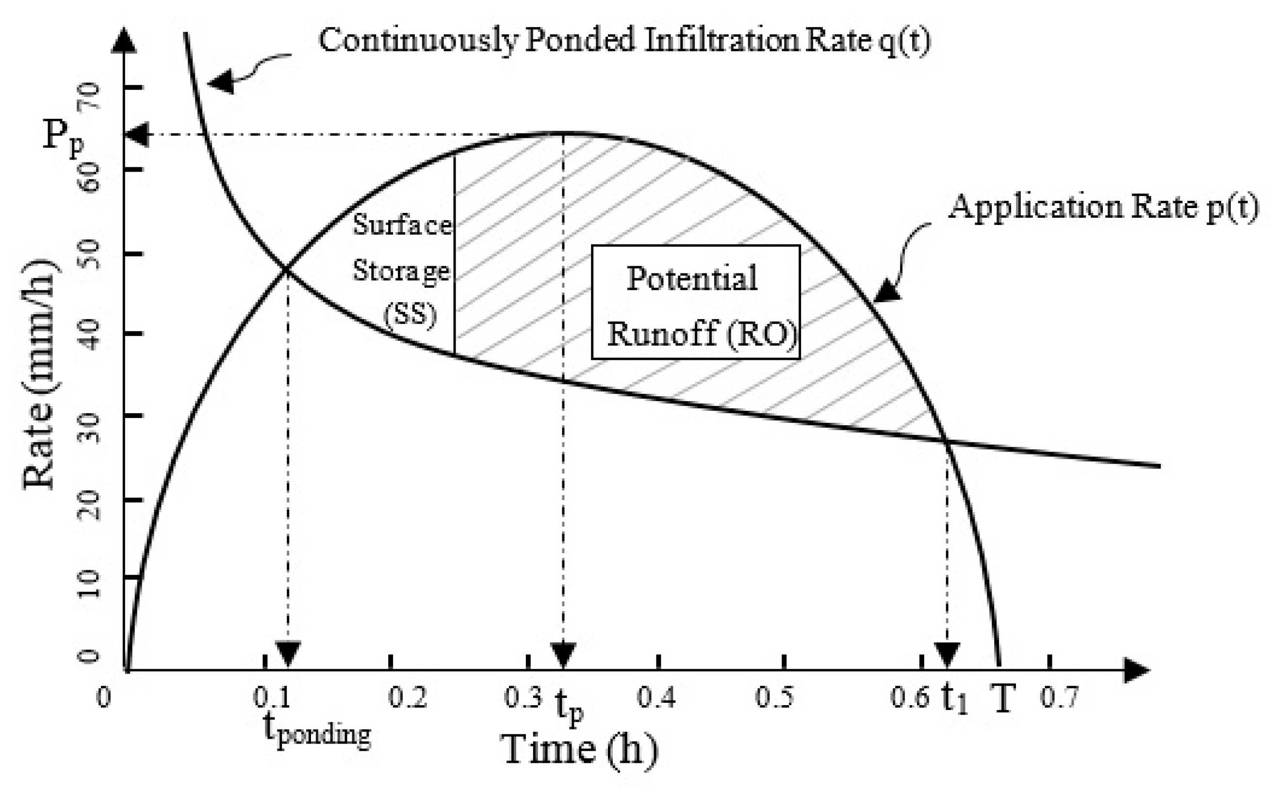
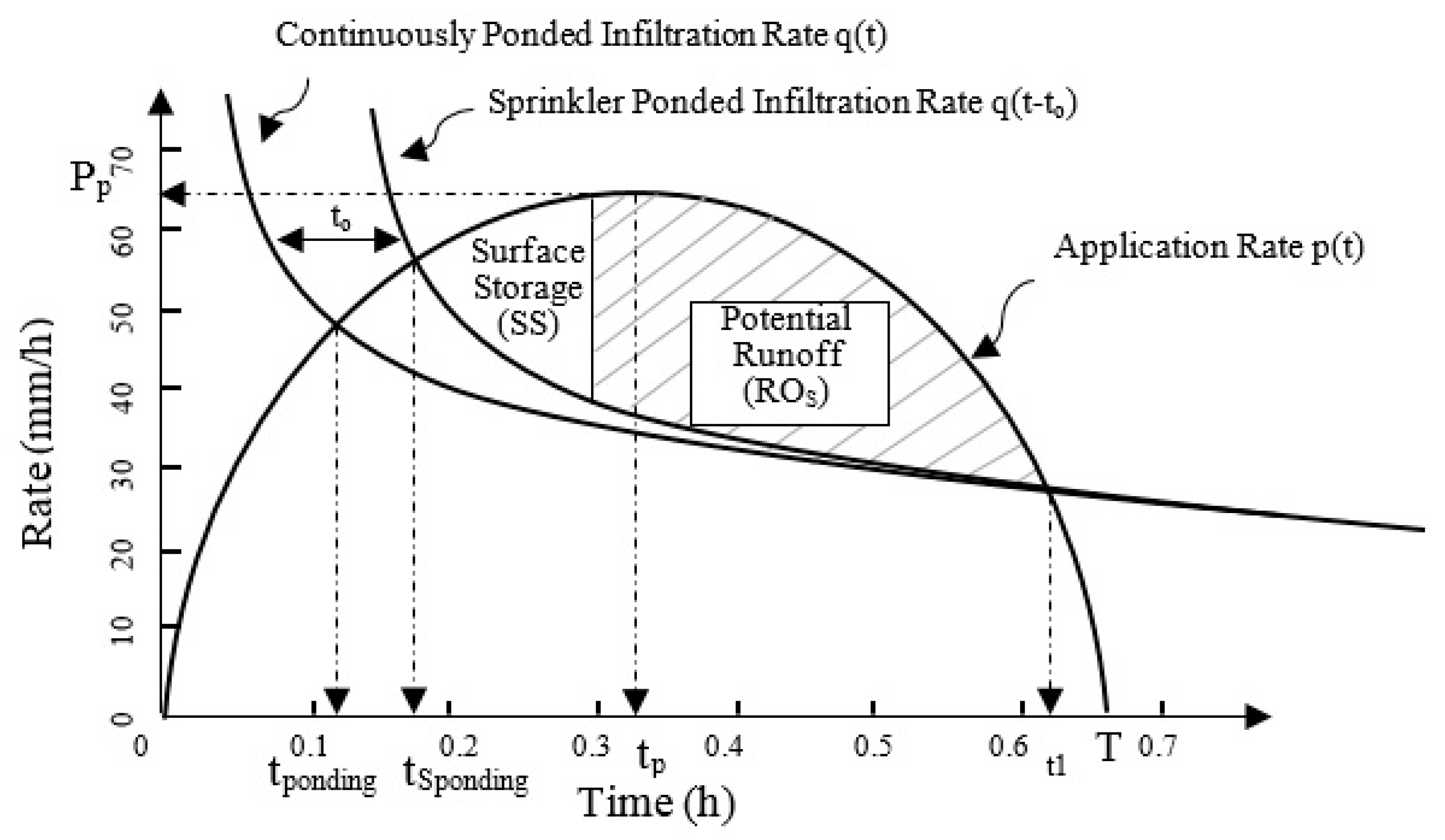
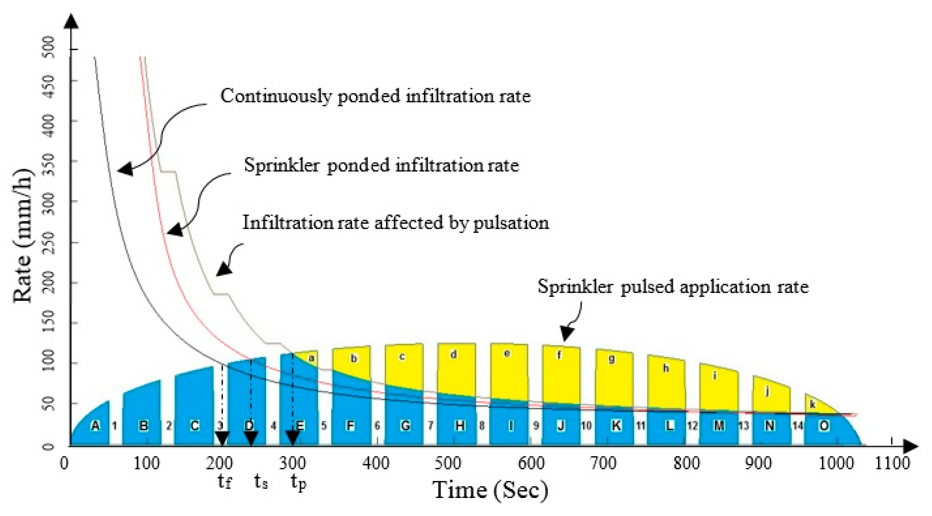
19]. For any sprinkler irrigation system, the surface runoff occurs when the water application rate exceeds the soil infiltration rate and the soil surface storage capacity [20,21]. The low-pressure sprinklers have a small wetting diameter, which results in a high instantaneous application rate and causes surface runoff on most of the soil types except soils with high intake rates [22,23]. Since the low-pressure sprinkler system has a high instantaneous application rate, the potential for increased surface runoff is higher [24].
Most researchers have reported that self-propelled sprinkler systems have the problem of surface runoff [25]. The magnitude of the runoff depends on several factors, such as irrigation machine characteristics, soil type, crop type, cultivation practices, and topography [26,27]. Ben-Hur, Plaut [28] and Letey, Vaux [10] suggested that crop yield can be affected by runoff in three ways: (1) The loss of runoff from the cultivated field is a loss of the water targeted for crop production; (2) the runoff will increase soil erosion and lead to a loss in fertiliser and nutrients that are washed out of the field; (3) the runoff water that accumulates in the low areas within the field will cause a poor distribution of water, reduce the water efficiency, and it can cause waterlogging that leads to either crop loss or a reduction in the crop yield. Kincaid, Heermann [22] concluded that 22% of the applied water was lost under high-pressure centre pivot sprinkler systems spraying a field with silty loam soil. Addink [23] noted that the runoff was 65% under a low-pressure sprinkler machine, while it was 22% under a high-pressure sprinkler system when irrigating a field with very fine sandy soil. Addink [23] and Kincaid, Heermann [22] reported that no runoff happened under both low-pressure and high-pressure sprinkler systems when irrigating a field with sandy soil.
Many studies have attempted to reduce surface runoff losses under the linear move sprinkler system by increasing soil infiltration rate and surface storage capacity through applying specific tillage practices or adding some materials to the soil surface [28,29,30,31,32,33,34]. These practices can decrease runoff volume to some extent, but they will not eliminate it. Other studies have focused on reducing either machine speed or sprinkler discharge rate to minimise surface runoff using different techniques [4,18,26,35,36,37,38]. However, the use of these methods often leads to a reduction in the applied depth for each pass of the irrigation machine, and the amount of the resulting runoff is not certainly at the lowest possible value. Also, some of these methods can affect the distribution uniformity and result in nonuniform water distribution, especially for low irrigation depths [39,40].
The efficiency of self-propelled sprinkler irrigation systems can be increased by decreasing runoff losses through matching the applied water volume and application rate to specific soil characteristics [39]. One of the methods used to increase the efficiency of self-propelled irrigation systems was to apply variable amounts of water along their lateral span and in the direction of movement to accommodate variable soil or crop conditions [40]. Variable-rate irrigation (VRI) technology has been used in precision irrigation. However, it is not a basic component in precision irrigation, but one of many other tools that might be suitable in the implementation of precision irrigation systems [41]. The potential for water saving by using precision or variable-rate irrigation can be achieved by: (1) not watering empty (uncultivated) areas inside the field; (2) decreasing irrigation to an amount suitable for specific problems, such as surface runoff, and matching the soil infiltration rate or different crop needs; and (3) fully optimizing and maximizing the economic value of the irrigation water [41].
For self-propelled irrigation systems, a variable rate has been achieved by: varying the ground speed of the system [26,38], changing the sprinkler nozzle bore by pulsing a retractable concentric pin in the nozzle bore over predefined duty cycles [42,43], or changing the ON time of individual or banks of nozzles of the sprinkler system [44]. Most researchers achieved variable water application by pulsing (opening) an individual or bank of solenoid valves for a part of the predetermined irrigation cycle (60 s or longer), to be compatible with a desired application rate [45,46]. The pulse modulation (on–off cycling of sprinkler valves) has become the most common industry standard technique used to control variable application rates [47]. Most research has used pulse modulation VRI to apply variable irrigation depths and hold the water from untargeted areas inside the field to overcome spatial differences in the water needs due to crop or soil variations [48]. However, there is very little research that has aimed to reduce surface runoff explicitly using the VRI technique, especially for the low-pressure sprinkler systems.
For VRI systems, application uniformity can be affected by sprinkler spacing, operating pressure, irrigation system component conditions, climatic conditions [49,50], and sprinkler height above the soil surface [51]. Some studies have reported a uniformity issue with VRI, especially with low application depths. Han et al. [52] measured the coefficient of uniformity (CU) under a linear move system supplied with VRI using the pulsing technique. The CU values for the variable application depths of 6, 13, 19, and 25 mm were 79.5%, 91.7%, 94.8%, and 94%, respectively. Their results showed that the uniformity decreased when applying lower depths. O’Shaughnessy et al. [48] performed uniformity tests (coefficient of uniformity (CU) and low quarter distribution uniformity (DUlq)) in the direction of travel of a centre pivot irrigation system by applying variable application depths using VRI with a pulsing technique. The mean values of CU and DUlq were between 86.3% to 89.5% and 76.3% to 82.9%, respectively, after applying irrigation depths in a range of 100%, 80%, 70%, 50%, and 30% from a 25-mm irrigation depth. The study highlighted a uniformity issue for the low pulsing rate, where the CU was decreased to 70% when applying a 30% pulsing rate (or depth = 7.6 mm) compared with pulsing rates >50%. Also, the DUlq was significantly decreased for the 30% pulsing rate compared with the higher pulsing rates.
Pulse modulation has become the industry standard [47]. However, most of the existing solenoids, pressure regulators, and valves can cycle between 250,000–300,000 times before breakdown [47]. Therefore, pulsing frequency (number of pulses) has become another major issue for the VRI technique when applying different targeted depths or application rates. However, considering lowering the number of pulses while applying variable irrigation depths has not been thoroughly investigated.
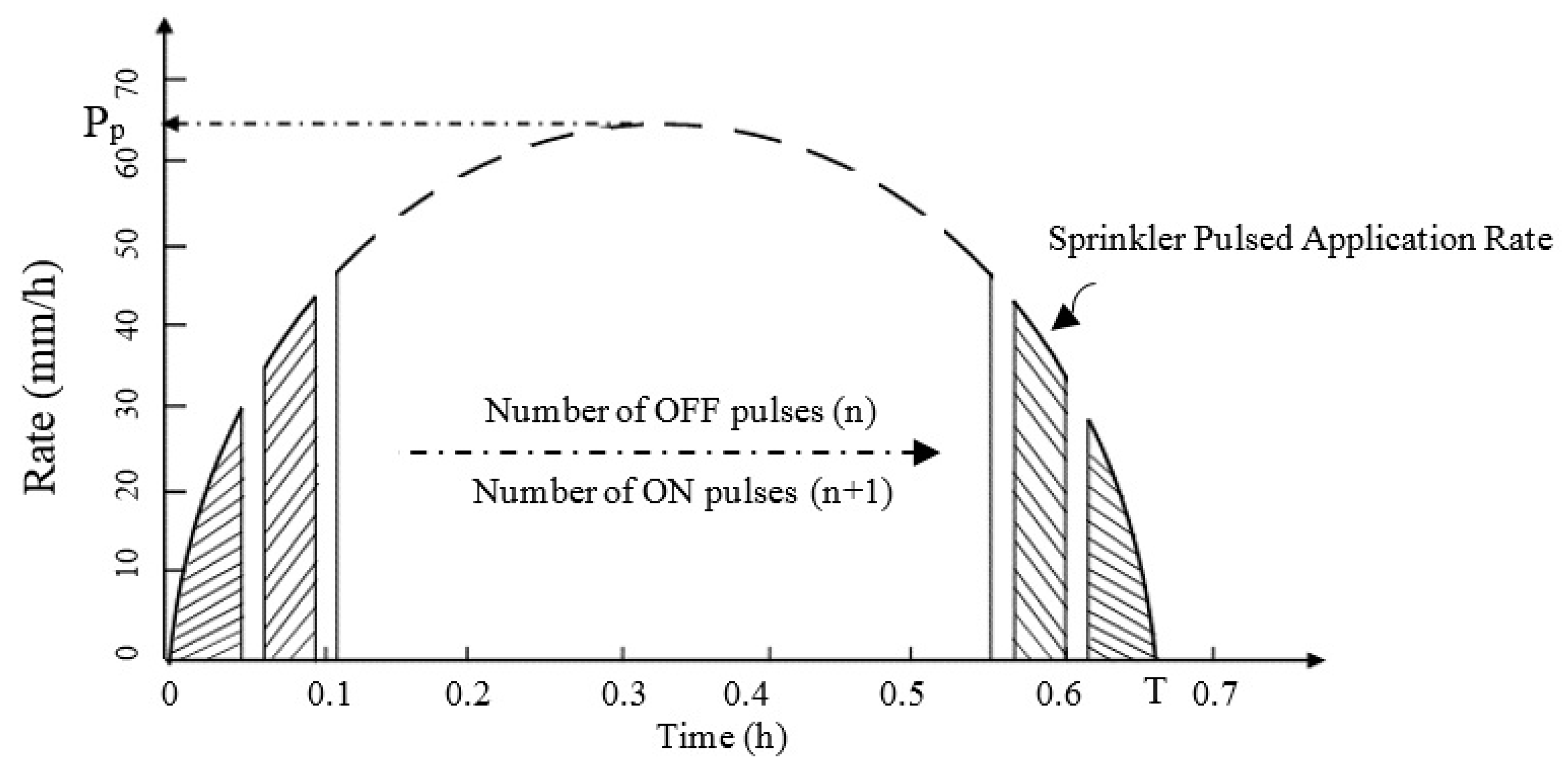
This research aims to develop a variable pulsed irrigation algorithm (VPIA) which is able to reduce surface runoff while delivering the highest irrigation depth under the linear move sprinkler irrigation system supplied with a Low Elevation Spray Application LESA using the ON–OFF pulsing technique. Also, it aims to assure a high distribution uniformity in the direction of movement with the lowest number of pulses to ensure the sustainability of the sprinklers’ mechanical parts.

2. Materials

The simulation tests of the variable pulsed irrigation algorithm (VPIA) were performed using a linear move irrigation system supplied with LESA sprinklers designed by Lindsay (LINDSAY CORPORATION, Omaha, Nebraska, USA). The specifications of the linear move irrigation system used in this study are listed in Table 1.
The soil type used in the simulation model was sandy loam soil, and the Philip’s two-term model was used to describe and simulate the infiltration rate and the accumulated infiltrated depth. The sorptivity (S) and the constant (A) in the Philip’s model for the sandy loam soil was obtained from the Green–Ampt infiltration parameters proposed by Rawls, Brakensiek [53] by applying the relations suggested by Rawls [54] and Philip [55] as follows:
S = ( 2 K s a t Δ θ | ψ f | ) 1 2
Δ θ = η θ 0
A = 0.38   K s a t
where: S is sorptivity in (cm/h0.5); Ksat is saturated hydraulic conductivity in (cm/h); |ψf|: is the wetting front soil suction head in (cm); η is the total porosity in (cm3/cm3); θ0: is the initial moisture content in (cm3/cm3); A is a constant in (mm/h).
On the assumption of Δθ = θe in Equations (1) and (2), the calculated parameters are listed in Table 2. It was assumed that the surface storage capacity is equal to (SS = 5 mm) in our algorithm.
A MATLAB code was written to apply the VPIA to the selected sprinkler system described in Table 1 to irrigate a field of sandy loam soil. The simulation tests were run under the assumptions of ideal weather conditions and bare soil irrigation, and evaporation and deep percolation losses were neglected. Every four sprinklers were assumed to be grouped and fitted with electric solenoid valves coupled to a programmable logic controller (PLC) to provide the variable pulse control. In practice, the PLC must receive the best solution of the number of pulses and the ON and OFF times from a remote computer through either a wired or wireless connection.

3. The Variable Pulsed Irrigation Algorithm (VPIA)

The lateral move sprinkler irrigation system supplied with LESA sprinklers was chosen because of its low water losses due to wind drift, droplet evaporation, and crop and soil surface evaporation. However, it might have a high runoff loss with some soil types due to its high instantaneous application rate. Therefore, the proposed variable pulsed irrigation algorithm (VPIA) based on the ON–OFF pulsing technique aims to reduce the runoff losses that resulted from using this system while delivering the highest possible irrigation depth. Also, it aims to maintain a good uniform water distribution in the direction of the movement.

3.1. The Required Data

Some factors related to the soil and the irrigation machine must be supplied to the algorithm as input data. According to the selected infiltration model, the soil data can be represented by the factors that describe the soil infiltration rate (q(t)), cumulative infiltration depth (I(t)), and the surface storage capacity (SS). The irrigation machine data can be represented by the factors that describe the water application rate (p(t)), as well as the maximum permissible pulse range (n) that the nozzles and its plates can tolerate to ensure the safety and sustainability of the sprinklers.
There are a lot of mathematical models that describe the infiltration rate q(t) and cumulative infiltration depth I(t), such as the Kostiakov, Horton, Holtan, Philip’s two-term, and Green–Ampt models [56]. The Philip’s two-term model was selected to represent the soil infiltration rate and cumulative infiltration depth in our algorithm because it is relatively simple, easy to use, reliable, and it does not require special equipment or complex calculations to obtain its factors. The following equations describe the Philip’s two-term model [55,57]:
q(t) = 0.5St−0.5 + A
I(t) = St0.5 + At
where: q(t) is the infiltration rate in (mm/h); t is the time for infiltration in (h); S is the sorptivity in (mm/h0.5); A is a constant in (mm/h); I is the cumulative infiltrated depth in (mm) at any time t.
The application rate p(t) of the irrigation machine is an important factor that affects the amount of runoff (RO) and must be calculated correctly. Its shape is elliptical and perpendicular to the lateral movement, as shown in Figure 1 [58]. The application rate is affected by the total flow rate (Q), machine speed (V), which is related to the targeted depth (Dg), and the sprinkler wetting radius (R). The following equations were used to calculate the application rate (P(t)), peak application rate (PP), time to reach the peak application rate (tp), and the time (T) that the machine takes to fully irrigate any point of the soil inside the field:
P ( t ) = P p t p 2   t   t p t 2
P p =   4 Q π R L
t p = R V
T = 2 t P
where: P(t) is the water application rate as a function of the time in (mm h−1); tp is the time after initial wetting at which the peak application rate is reached in (h); Pp is the peak application rate for the elliptical pattern of the sprinkler package in (mm h−1); Q is the total flow rate of the machine in (L/min); R is the wetted radius of the sprinkler in (m); L is the machine length in (m); V is the average travel speed of the lateral in (m/min); and T is the time the machine takes to fully irrigate any point of the soil inside the field.

3.2. Computational Investigation for Runoff Potential

The soil infiltration rate and sprinkler application rate of the irrigation machine are both important factors that affect the amount of runoff and must be determined correctly. The sprinkler application rate may exceed the soil infiltration rate because the latter decreased through time due to the increase of the soil water content; at this point, the water will accumulate on the soil surface and results in ponding. The water ponding starts when the application rate p(t) overrides the soil infiltration rate q(t) at a point of time called tponding, as shown in Figure 1. The soil surface can temporarily store some of the excess water; this is called surface storage capacity (SS). As soon as the local surface storage (SS) is filled, the excess water will start to flow over the field as runoff losses (RO). The potential runoff (RO) is represented by the dashed area shown in Figure 1 [58].
Usually, the infiltration rate is measured using an instrument called an infiltrometer. According to the principle of operation of the infiltrometer, it can be categorized into two different types: the flooding type and the sprinkling type. The flooding devices are much more widely used than the sprinkling type because their installation and use are easier and require less equipment. The infiltration rate resulting from the use of flooding infiltrometers represents the continuously ponded infiltration rate as shown in Figure 1. However, the water application rate for the linear move sprinklers at a given point rises and then drops, instead of being constant as in the flood irrigation or stationary sprinklers. Therefore, the prediction of runoff volume and ponding time will not be accurate if the continuously ponded infiltration rate curve is superimposed over the water application rate curve of the moving sprinklers machine. So, the sprinkler ponded infiltration rate must be used instead of the continuously ponded infiltration rate, as shown in Figure 2.
The sprinkler ponded infiltration rate curve is calculated using an implicit equation that describes the infiltration rate (q) in terms of cumulative infiltrated depth (I) rather than time (t), as described by [59]. For a given cumulative infiltrated depth (I), the infiltration rate (q) can be calculated as follows:
q ( I ) = A + A S S 2 + 4 A I S
According to Tarboton [59], the soil infiltration rate stages can be classified into three stages depending on the water input rate: prior to ponding, at ponding, and after ponding. For a given water input rate (p), the cumulative infiltrated depth before ponding can be calculated as the area under the water input curve, or (I = p × t). When the water input rate (p) increases to the point where it equals the decreased infiltration rate (q), i.e., q = p, ponding occurs. The Philip cumulative infiltration depth at ponding can be determined by substituting q = p into Equation (10) as follows:
I p o n d i n g =   S 2 ( p     A 2 ) 2 ( p     A ) 2
The Philip time to ponding equation will be as follows:
t p o n d i n g = I p o n d i n g p =   S 2 ( p     A 2 ) 2 A ( p     A ) 2
The infiltration that occurs after ponding can be found by shifting the infiltration rate under ponded conditions by (to), as shown in Figure 2, where the cumulative infiltration (I) (in Equation (5)) equals the initial cumulative infiltration (Is) at time (ts). Therefore, (to) can be calculated as follows:
t o = t s 1 4 A 2 ( S 2 + 4 A I s S ) 2
Then, the Philip cumulative infiltration depth after ponding can be obtained by using the following equation:
I(t) = S (t − to) 0.5 + A (t − to)
The equation of (I = p × t) is applied when the water input rate is constant. However, the sprinkler application rate P(t) is not constant, as it increases until it reaches a maximum at a certain point in time, and then decreases in a nonlinear manner as the sprinkler moves over the measuring point. Therefore, a hyetograph approximation for the sprinkler application rate is used to overcome this issue and estimate the sprinkler ponded infiltration rate curve. Through the MATLAB code, the sprinkler application rate will be divided into small equal time intervals (m steps), making it like the precipitation hyetograph as shown in Figure 3. The application rate for each step will be considered as a constant rate with its peak value equal to the integration value of the area under the sprinkler application rate curve for this interval. The time interval for the steps will affect both the number of steps (m) and the computational accuracy; i.e., a smaller step time will result in both high computational accuracy and high number of steps, and vice versa. However, the runtime for the calculations will be affected directly by the number of the steps; i.e., the higher the steps’ number, the higher the computational runtime. Therefore, the number and time of each step must be carefully determined to achieve the best requirements in terms of computational accuracy and operating time. In our algorithm, the step time was chosen to be 2 s to obtain a higher mathematical resolution.
According to the machine speed, the sprinkler ponded infiltration rate curve is calculated and the potential runoff (ROS) related to the specified soil type is determined by applying the steps described in [59]. The results will be arranged in a table called the runoff potential table (RPT) to show at which speed the runoff starts with its amounts calculated from the applied irrigation depth (dg) and the actual infiltrated depth (I).

3.3. The Principles of the VPIA

The VPIA must be applied when the runoff volume exceeds the allowable runoff threshold. In the VPIA, the runoff threshold is assumed to be 1% from the applied depth. A graphical method will be used to explain how the variable pulse algorithm works, and the following steps will be applied to reduce the runoff by adjusting the number of pulses and the width of each pulse:
(a)
Choosing the speed range where runoff occurs from the runoff potential table (RPT), and for each selected speed, the total irrigation time (T) shown in Figure 1 must be calculated. T depends on the speed of the machine (V) and the wetting radius of the sprinkler (R) and can be calculated using Equation (9).
(b)
From the manufacturer specification sheet of the sprinklers, specify the range of the maximum permissible pulses (n: pulses per minute) and the minimum and maximum time for the OFF and ON pulses that the sprinkler nozzles and plates can endure, in order to assure the equipment safety and sustainability.
(c)
For the selected speed, the total time (T) will be divided into (n + 1) equal ON pulses and (n) equal OFF pulses. The sequence of pulses starts with the ON pulse and then alternate with OFF pulses, ending with an ON pulse. Therefore, the first pulse in the sequence will be ON and the last pulse will be ON as well. So, the suggested new shape of the application rate will be represented graphically by a pulsed application rate curve where the ON pulses are represented by the dashed areas and the OFF pulses are represented by the blank areas, as shown in Figure 4.
(d)
According to the suggested algorithm, the reduction of the runoff losses will be achieved initially by controlling the number of OFF pulses, starting with the lowest number of pulses that the sprinkler can endure (2 OFF pulses and 3 ON pulses, as suggested by the algorithm), until the maximum allowable number of pulses is reached (50 OFF pulses and 51 ON pulses, as suggested by the algorithm); and then by controlling the width of the OFF pulses for each selected number of pulses, by starting with the lowest value of OFF pulses (2 s, as suggested by the algorithm) until reaching the allowable value of OFF pulses that assures zero runoff at the first soil point in the direction of the machine movement, considering the surface storage capacity.
(e)
The cumulative infiltrated depth I(t) along with the soil infiltration rate q(t) and the runoff (RO) will be calculated by using Equations (10)–(14) and by following the steps described by Tarboton [59], considering the new pulsed application rate. The calculation of I(t), q(t), and RO is affected by pulse status and the ponding stage. Therefore, these calculations will contain three stages: before the ponding, at the ponding, and after ponding. Assuming the pulsed application rate described in Figure 4, the calculation stages will be described as follows:
1. 
Before ponding stage: In this stage, the soil infiltration rate exceeds the application rate, so there will be no runoff during this period. Therefore, all the applied water volume during the ON pulses will infiltrate and contribute to the cumulative infiltrated depth (I). For every ON pulse, the cumulative infiltrated depth (I) will be calculated first, and it will increase gradually as it is equal to the summation of the areas under the application rate curve (blue areas: A–D and part of E). During the OFF pulses (blank areas 1–4), the cumulative infiltrated depth (I) will not change and will stay constant. On the other hand, the soil infiltration rate (q) will be calculated depending on the cumulative infiltrated depth (I) amount by using Equation (10), where (q) will decrease during the ON pulses and remain constant during the OFF pulses, as shown in Figure 5.
2. 
At ponding stage: This stage represents the first time when the application rate equals the soil infiltration rate. When the water input rate increases to the point where it equals the decreased infiltration rate, ponding occurs. At this stage, the cumulative infiltrated depth (I) will be calculated using Equation (11) and the ponding time will be calculated using Equation (12). The important point here is that the ponding time will be affected by the pulsing and will be shifted more to the right, which decreases the potential runoff area as shown in Figure 5, where tf: ponding time under continuously flooded condition, ts: ponding time under sprinkler condition, and tp: ponding time under pulsed condition.
3. 
After ponding stage: In this stage, the application rate exceeds the infiltration rate, and the excess water volume during the ON pulses will accumulate over the soil surface as shown in Figure 5 (yellow areas). During each ON pulse, if the volume of accumulated water (yellow areas) exceeds the surface storage capacity (SS), then the difference between the accumulated water over the soil surface and surface storage capacity (SS) will be considered as a runoff loss. The OFF pulses in this stage will contribute to reducing the runoff losses by giving time for the accumulated water (yellow areas) to infiltrate into the soil. If the total water volume of any of these areas does not infiltrate during the next OFF pulse, it will be added to the residues from other quantities from previous areas. During each addition of the residual water from the previous step, if the water volume that accumulates over the soil surface exceeds the surface storage capacity, the excess water will be lost as surface runoff.
During the ON pulses, the cumulative depth (I) resulting from the previous stages will increase with the summation of the areas under the soil infiltration rate curve (blue areas: part of E, F, G, H, …, O) as shown in Figure 5. During the OFF pulses, all or part of the water volume that accumulated over the soil surface (yellow areas) will infiltrate and contribute to the cumulative depth (I), causing an increase of its amount. The soil infiltration rate (q) will be calculated depending on the cumulative infiltrated depth (I) by using Equation (10), and it will decrease during the ON pulses. However, due to the infiltration of all or part of the surface storage amount (yellow areas: a, b, c, d, …, k) during the OFF pulses, the soil infiltration rate (q) decreases as well, as shown in Figure 5.
If the accumulated water over the soil surface (one or all the yellow areas) fully infiltrates into the soil before the end of the OFF pulse, then the infiltration rate will drop to a certain point at the time when the accumulated water has thoroughly infiltrated, and then continue as a constant rate. This case is shown in Figure 5 between the E and F ON pulses, when the amount of the accumulated water over the soil surface (yellow area (a)) has infiltrated completely before the end of the 5th OFF pulse.
At the end of the pulse sequence, if the amount of the accumulated water over the soil surface (the sum of the residual water volume from the yellow areas) is less than or equal to the surface storage capacity (SS), then it will remain over the soil surface and it will later infiltrate into the soil and contribute to the cumulative infiltrated depth (I). Otherwise, the difference between the accumulated water over the soil surface and surface storage capacity (SS) will be considered as a runoff loss and it will be added to any runoff losses produced from previous steps (RO).
(f)
The OFF pulses will have a significant impact on reducing runoff losses, because first, they reduce the amount of the supplied water, and second, it gives extra time for the surface water (accumulated water over the soil surface) to infiltrate into the soil. However, a sort of balance between the surface runoff volume and the amount of the infiltrated depth must be achieved by selecting the appropriate number and width of the OFF pulses to achieve this balance. Therefore, several cases will be studied with different numbers of OFF pulses, starting from two OFF pulses and three ON pulses as a first case. Then, we proceed with the cases by increasing the number of OFF pulses by one pulse gradually until the maximum allowable amount of pulses (n) is reached. Note that the number of ON pulses will also increase. The maximum number of allowable pulses is assumed to be 50 pulses in our algorithm.
(g)
In each case, there are several steps, and the number of steps is associated with the time of the OFF pulses that make the amount of runoff at the first point of soil in the direction of motion equal to zero. For the first step of each case, the OFF pulses’ duration will start at the minimum value of 2 s, and the ON pulses’ duration will be set to the total time (T) using the following equation:
T = n*TOFF + (n + 1) *TON
(h)
For the first case, which contains two OFF pulses and three ON pulses, starting with the first step where the time of the OFF pulses is two seconds (TOFF = 2 s), the cumulative infiltrated depth (I) and runoff (RO) will be calculated as described in point (e). If the runoff is not equal to zero (RO ≠ 0), then we will go to the second step by increasing the duration of the OFF pulses by one second (TOFF = 3 s), and accordingly, the ON pulses’ duration will be recalculated using Equation (15). The same calculation of I and RO will be repeated for this step. If the runoff is still not equal to zero, then the steps will continue by increasing the duration of the OFF pulses by one second for each step until one of the following conditions is satisfied:
(1)
The runoff is equal to zero (RO = 0), or
(2)
The maximum or minimum allowable duration of the OFF or ON pulses has been reached.
The values of the OFF and ON duration that satisfy either of the previous conditions will be chosen as the best solution for this case.
(i)
The second case will contain three OFF pulses and four ON pulses, and the third case will contain four OFF pulses and five ON pulses, and so on for the subsequent cases until the maximum number (n) of the OFF pulses has been reached. For each case, the same procedure listed in step(h) will be followed until one of the conditions is satisfied, and the time of the OFF and ON pulses that meets these conditions will be chosen as the best solution for each case.
(j)
After completing all the cases, the results will be arranged and stored in a table called the runoff solution table (RST). These results represent the best solutions of the number of pulses and the ON and OFF widths that give either zero or the lowest runoff volume with the corresponding cumulative infiltrated depth for the first point (X1) of the soil in the direction of the movement inside the field.
(k)
Due to the pulsation effect, the sprinklers will not spray the water continuously, and this will affect the water distribution uniformity, especially for the successive soil points in the direction of the machine movement. According to our algorithm, the sprinkler application pattern will be changed to the suggested new pattern as shown in Figure 4. Because of this change, each successive point in the direction of movement will receive a spray pattern different than for the first point. Also, because of spatial difference between the successive soil points, a time shift for the sprinkler pattern between these points will occur and it is mostly related to the machine speed.
(l)
Since all the solutions that are listed in the RST result from applying the algorithm to a single test point (first point in the direction of movement (X1)), another test must therefore be carried out for the successive points (X2 – Xi) to check the distribution uniformity and the runoff potential when applying each solution from this table. To do such a test, the following procedure will be applied:
  • Several hypothetical test points Xi (like the principle of catch cans) should be distributed in one line parallel to the direction of the machine movement, as shown in Figure 6. The suggested number of these points (i) depends on the width of the sprinkler wetting diameter, while the suggested distance between them depends on the required level of calculation accuracy.
  • The pulsed application pattern for each case listed in the RST will be applied to the successive points. This pulsed application pattern must be reshaped for each test point by considering the effect of the time delay between these points related to the specified machine speed.
  • The amount of runoff (ROi) and the cumulative infiltrated depth (Ii) for each successive point (Xi) shall be calculated by following the procedure described in step (e), considering the new reshaped pulsed application pattern. The results will be listed in a new table called the uniformity check table (UCT). The values of the runoffs (ROi) and the cumulative infiltrated depths (Ii) for all the successive points will be averaged and listed in the UCT as well.
  • The standard deviation test will be applied to cumulative infiltrated depths (Ii) for all test points to check the degree of the distribution uniformity for all the cases listed in the UCT.
(m)
To select the unique, best solution among all the solutions listed in the UCT, the following criteria will be applied:
  • To achieve the main goal of this research, reducing runoff losses, the cases that have an average runoff volume higher than the accepted threshold will be excluded. In our algorithm, the runoff threshold will be set to 1% from the applied depth.
  • Among the remaining cases after applying the first criterion, to assure a high degree of distribution uniformity in the direction of movement, the cases that have a standard deviation higher than the accepted threshold will be excluded. In our algorithm, the allowable variance between the highest and lowest infiltration depths for the successive points will be taken as 1% of the applied depth.
  • The remaining cases after applying the previous two criterions will be arranged according to their infiltration depth in descending order along with their corresponding values of pulse number and width. Therefore, the case with highest depth will be the first in the new list. To ensure delivering a high depth of water to the soil for the selected speed, all cases with a depth below 1% of the highest depth will be excluded.
  • To decrease the wear of sprinklers and reduce maintenance costs and extend the life of the mechanical parts, the case with lowest number of pulses among the cases resulting from applying the third criterion will be chosen as the best unique solution for the specified speed.

4. Simulation Results

To examine the performance of the proposed algorithm, we simulated the soil infiltration rate and the machine application rate before and after pulsing using a code written in MATLAB software. The MATLAB code was written to apply the VPIA on the selected sprinkler system described in Table 2 to irrigate a field of sandy loam soil. The code consists of four steps: In the first step, for each speed of the irrigation machine, the surface runoff potential will be checked according to the sprinkler ponded infiltration rate that corresponds to the application rate of the specified speed. The results of the runoff for each speed will be stored in a table called the runoff potential table (RPT). The second step comprises the calculation of the RST, which contains the best solutions of the number of pulses and the ON and OFF widths for the speeds at which the runoff exceeds the allowable threshold which is listed in the RPT. In the third step, for each result listed in the RST, a distribution uniformity and runoff check are performed for the successive test points, and then the UCT is created. The final step is to select the best solution among all the solutions that resulted from the previous two tables according to the selection criteria. The results of each step will be stored in Excel spreadsheets for easy access to be retrieved for further calculations.
Since the irrigation machine has a range of speeds, the algorithm will be applied for the speeds at which the runoff exceeds the allowable threshold. The runoff threshold is set to 1% from the applied depth in our algorithm. Therefore, the runoff losses (ROs) along with the supplied irrigation depth (dg) and the infiltration depth (I) for the speed range of the irrigation machine used were calculated and listed in the runoff potential table (RPT) as shown in Table 3.
From the RPT, it seems that the runoff starts when applying an irrigation depth of ≥20 mm. Therefore, the VPIA will be applied to all the speeds that have resulted in an amount of runoff that exceeds the threshold of 1% from the applied depth. Working on the first speed of 25 m/h to apply a 20 mm irrigation depth, the generated runoff was (1.55 mm > threshold (0.2 mm)), and the total time (T) that the machine needed to irrigate any single point of the soil was (T = 733 s). Therefore, the application rate will be pulsed within this time using several pulsing cases, starting with the first pulsing case (Case 1), in which the application rate will be pulsed with 2 OFF pulses and 3 ON pulses. In each case, a wide range of steps with different pulse widths will be tested, where the time of the OFF pulses will start from (TOFF = 2 s) as a first step, and the steps will continue by increasing the time of the OFF pulses by one second for each next step until the runoff is equal to zero, considering that all these calculations are made for the first test point (X1) by applying the new intermittent application rate. Also, the amount of surface storage capacity (SS = 5 mm) is considered when calculating the surface runoff and the actual infiltration depth. The results of these calculations are presented in Table 4, where the applied depth was 20 mm and the infiltrated depth before pulsing was 18.45 mm with 1.55 mm of runoff, considering a surface storage capacity of 5 mm.
From Table 4, it is shown that for Case 1, it took 28 steps to get zero runoff, with TOFF = 29 sec, TON = 225 sec, and infiltrated depth I1 = 18.128 mm as a solution for zero runoff for this case. In our algorithm, we suggested that the maximum allowed number of OFF pulses is 50 pulses, which the user can change to match the sprinkler and nozzle specifications. Therefore, the same calculations were repeated for the other 48 cases, and the results of all the solutions that give zero runoff were listed in the RST. The RST is shown in Table 5, where the applied depth was 20 mm and the infiltrated depth before pulsing was 18.45 mm with 1.55 mm of runoff, taking into account a surface storage capacity of 5 mm.
The solutions listed in Table 5 represent the best solutions for different pulse numbers that gives zero runoff for the first test point (X1). Since the time shift between the successive test points will cause a reshaping and shifting in the new pulsed application rate, it will result in variations in the runoff and infiltration depth values for each test point. Therefore, the next stage in the algorithm is to check the runoff and the distribution uniformity when applying the new pulsed application rate for each of these solutions to the successive test points in the direction of movement.
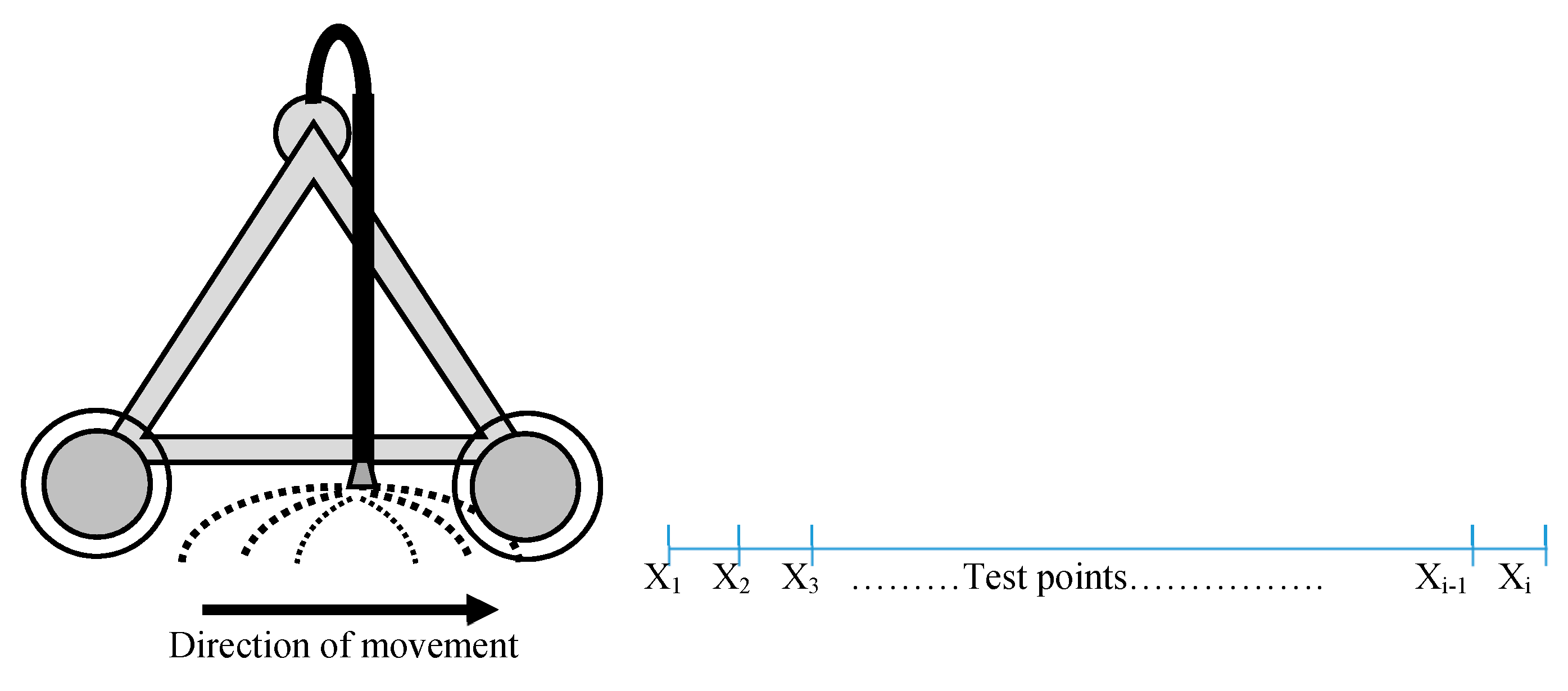
Since the pulsing will affect the application pattern, hypothetical test points must be used to check the runoff losses and the distribution uniformity for the successive points in the direction of movement. The number of the test points and the distance between them depends on the sprinkler wetting diameter and the aimed level of accuracy for the calculations. According to the sprinkler wetting diameter (5.2 m) of the system used, 22 test points (X1- X22) are suggested to be used and placed in one line in the direction of movement. These points were spaced 0.25 meters apart along the line, as shown in Figure 6, except the last point was placed at 0.2 m distance from the previous point to match the width of the wetting diameter.
Starting with the first solution of Case 1 that is listed in Table 5 (number of OFF pulses = 2, TOFF = 29 s, TON = 225 s), the runoff and infiltration depths were calculated for all other 21 test points after applying the new and shifted pulsed application rate. The new results were arranged in another table, as shown in Table 6. The average of runoffs and depths for the test points along with the standard deviation of the depths were also be calculated and listed in the same table (Table 6). The same calculation procedure was repeated for all the cases listed in Table 5, and the results were arranged and listed in the UCT as shown in Table 7.
The final stage of the VPIA is to apply the selection criteria to choose one unique solution among the solutions listed in the UCT (Table 7) for the selected speed of 25 m/h. By applying the first criterion, the following cases were excluded because they have an average runoff higher than 0.2 mm: Case 1, Case 2, and Case 3. From the remaining cases, the following cases were excluded because they did not satisfy the uniformity distribution criterion: Case 4 and Case 6. According to the infiltrated depth, the cases that were left after applying the previous two criterions were ordered in descending order along with their corresponding pulse number and width. Since Case 32 has the highest infiltration depth of 18.230 mm, it will be the first case in the new list. To apply the third criterion, the new infiltration depth threshold was set at 1% lower than the highest depth of 18.230 mm, which becomes 18.048 mm. Therefore, all cases that have an infiltration depth lower than 18.048 mm were excluded. The remaining cases with their corresponding details are listed in Table 8. All the solutions listed in Table 8 are good solutions that give low runoff and uniform depth along the direction of movement. However, we must select only one solution among these solutions. Therefore, to select a unique solution among all the listed solutions in Table 8, the fourth criterion was applied by selecting the case with lowest pulse number, which was Case 5 with the following factors: number of OFF pulses: 6 pulses, TON = 96.14 sec, TOFF = 10 sec. Therefore, for the selected speed of 25 m/h, when applying Case 5 factors to generate the pulsed application rate, the new average runoff decreased from 1.55 mm to 0.144 mm, while the new average delivered infiltration depth decreased from 18.45 mm to 18.20 mm.
The VPIA will be applied to all other speeds that generate a runoff higher than the threshold values. Table 9 shows the best solutions for these speeds after applying the VPIA.

5. Discussion

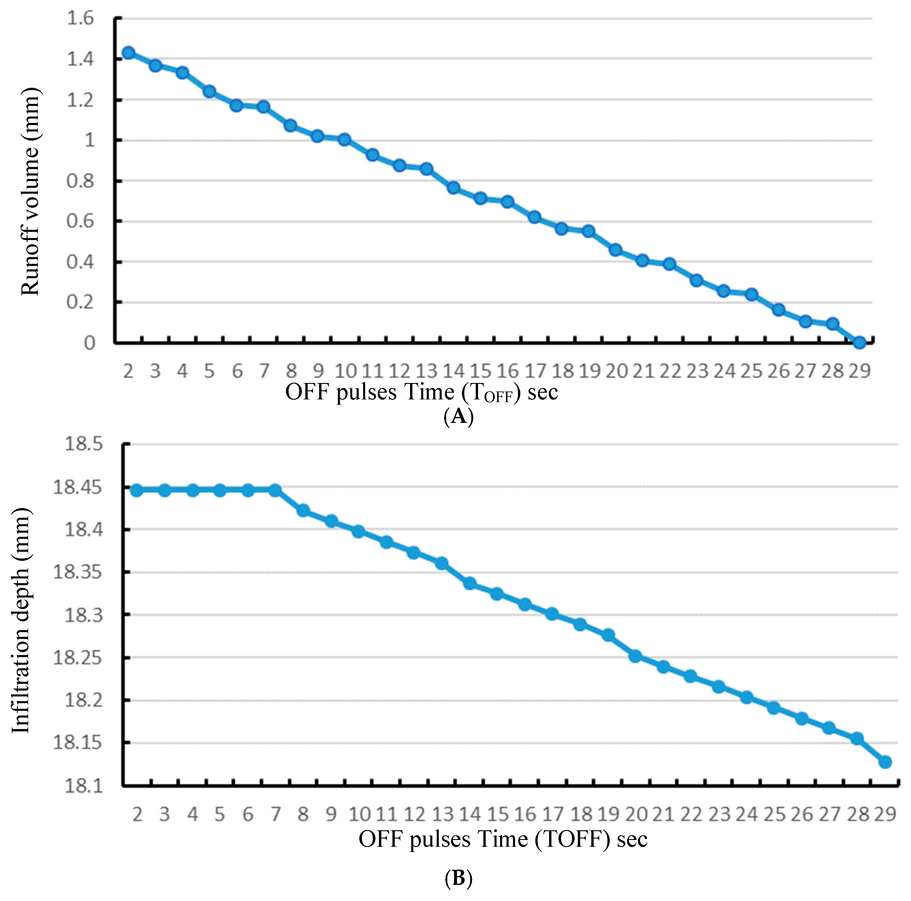
According to the VPIA, the runoff reduction is controlled by the number and the width of the OFF pulses within the total time (T). Regarding the results listed in Table 4 for the first test point, Figure 7A shows that for the specified case (Case 1) with a fixed number of OFF pulses (2 OFF pulses), the runoff was reduced by gradually increasing the width of the OFF pulses until it reached a zero value. However, the infiltration depth for the same point will decrease because of increasing the width of the OFF pulses, as shown in Figure 7B. From these results, we conclude that the OFF pulses’ width had two impacts: first, it decreased the amount of the applied water, and second, it gave more time for the accumulated water to infiltrate into the soil. Therefore, increasing the width of the OFF pulses will positively decrease the runoff volume, but on the other hand, will reduce the infiltrated depth.
For the first case, the number and width of the OFF pulses that make the runoff for the first test point equal zero was selected as the best solution for this case. Since the application rate pattern was altered by the pulse effect, successive test points in the direction of movement received a quantity and pattern of water that differs from the first test point. This may lead to an uneven distribution of water in the direction of movement and increase the possibility of runoff for these points. Therefore, to check the uniformity and the runoff potential for the selected case, the infiltration depth and the runoff must be calculated for each test point by using the same calculation procedure that was applied on the first test point, considering the changes in the application rate pattern for every test point.
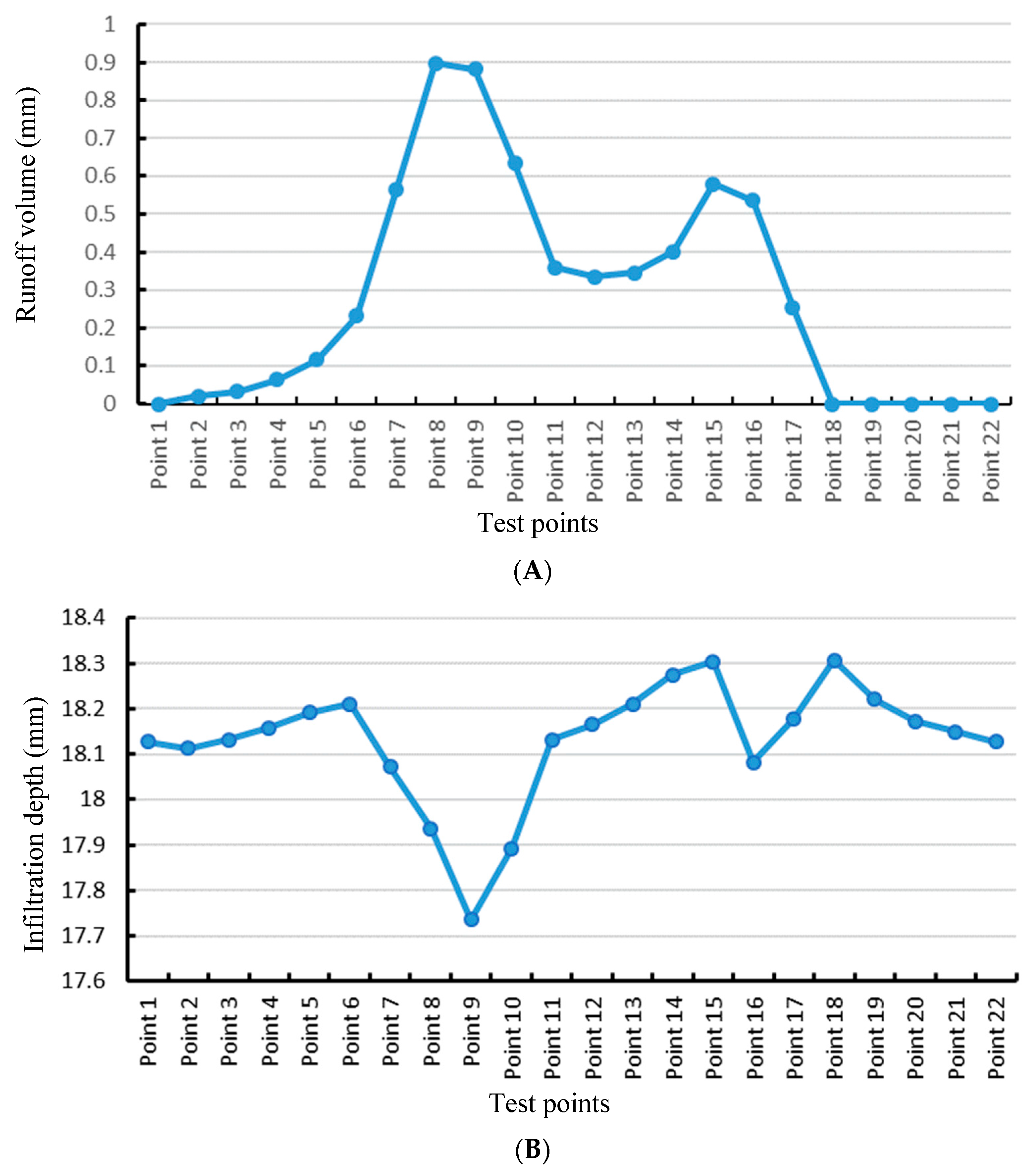
Figure 8A shows the runoff potentials when applying the pulsed application rate (resulting from the first test point in Case 1) to the successive test points using the results listed in Table 6, while the infiltration depths for the successive test points after applying the same pulsed application rate is shown in Figure 8B. From Figure 8A, it is obvious that the Case 1 solution was not a good solution as it w caused an undesirable amount of runoff (>0.2 mm) for several of the successive test points, even if it gave zero runoff for some of the others. Also, this solution led to unequal distribution of water for the successive test points, as shown in Figure 8B. Therefore, we must try other case solutions by increasing the number of the OFF pulses and repeating the same procedures. Finally, we must choose one from all the solutions that satisfy the selection criteria.
The final solutions for the different machine speeds listed in 
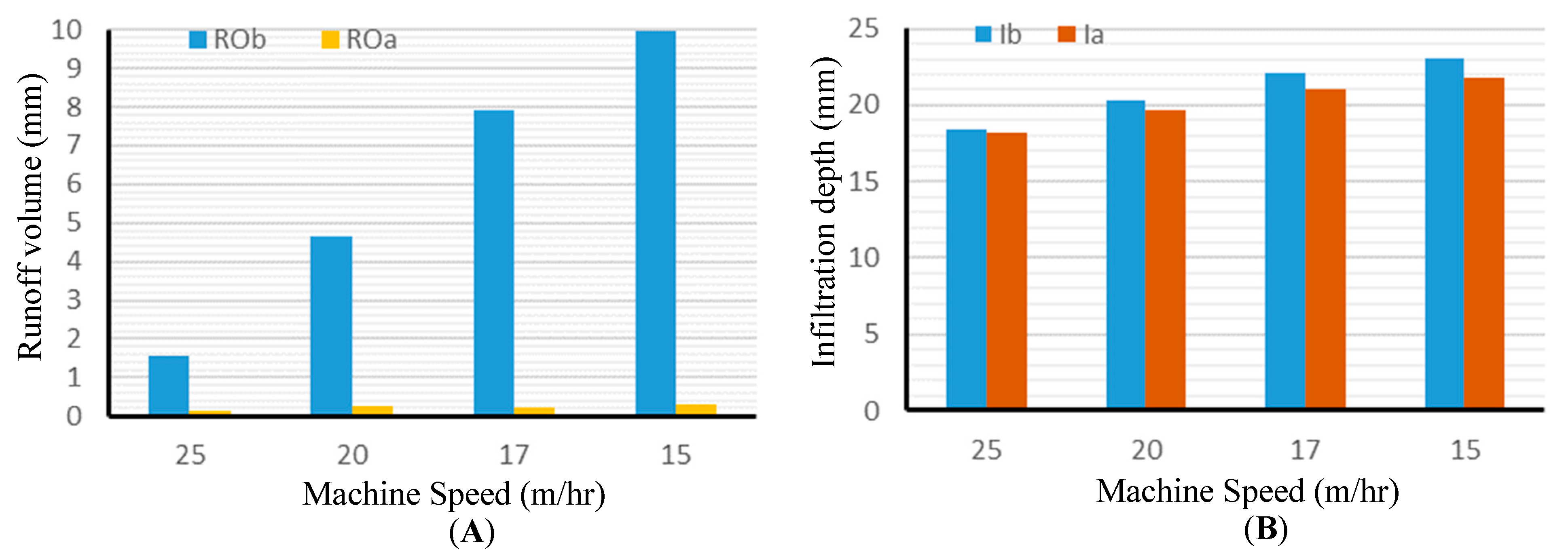
Table 9 show that our proposed algorithm has reduced the amount of runoff by 90.7%, 94.65%, 96.98%, and 96.94% for the applied depths of 20 mm, 25 mm, 30 mm, and 35 mm, respectively. Also, Table 9 can be considered as a look-up table (i.e., for every machine speed, the computer will directly select the solution that gives the best results from this table). Figure 9A shows a comparison between the runoff before pulsing (ROb) and after pulsing (ROa) for different machine speeds. Although the delivered average irrigation depth using the VPIA was slightly decreased compared with the normal continuous application rate, the VPIA achieved the delivery of an acceptably high irrigation depth with very low runoff losses. Figure 9B shows a comparison between the average infiltration depth before pulsing (Ib) and after pulsing (Ia) for different machine speeds. The results also show that the proposed VPIA maintains a uniform distribution of water in the direction of movement. The uniformity of water distribution and the runoff have a direct impact on the crop growth, crop yield, and soil and water resource sustainability. Therefore, the VPIA allows the irrigator or the farmer to specify the threshold for the acceptable runoff and the level of uniformity according to their experiences about the impact of these factors on the crop growth and resource sustainability.

6. Conclusions

The proposed VPIA to reduce runoff losses under a low-pressure lateral move irrigation machine was evaluated using a MATLAB simulation code. The simulation results demonstrated that the VPIA is efficient in reducing the runoff losses while delivering a high irrigation depth with a high level of distribution uniformity with the lowest pulse numbers. The results showed a runoff reduction of at least 90.7% by applying pulsing compared with irrigation under the same conditions without pulsing. A high level of distribution uniformity in the direction of movement while delivering the highest possible irrigation depth using the lowest number of pulses was also achieved. Also, the results revealed that the number and width of the OFF pulses and their location within the total time (T) of the application rate have a significant impact on the amount of runoff and the uniformity of water distribution in the direction of movement. Thus, the selection of the number and width of the OFF pulses and their distribution within the total time (T) according to the proposed algorithm, rather than assigning the OFF pulses with a specific percentage from a fixed cycle time (as other researchers have done), led to reducing the runoff to a low value and obtaining a high level of distribution uniformity. Overall, the evaluation proved the VPIA has provided a consistent manner in selecting the pulse numbers and widths to achieve the desired irrigation depth and runoff losses under the low-pressure sprinkler irrigation machine. Thus, this method can be considered as a new method in terms of selecting the width and number of pulses compared to other research and studies in this field. This paper represents the basic step in our research, and the work is proceeding in testing the proposed algorithm to apply variable-rate irrigation and investigate its impact on delivering low irrigation depth while achieving high distribution uniformity.

Author Contributions

All authors contribute equally.

Acknowledgments

A.A.A.A.-B. would like to thank the Iraqi Ministry of Higher Education and Scientific Research (MOHESR), University of Baghdad (UoB), for sponsoring this work. We thank Aaron Sauser and Erick Hernandez from Lindsay Corporation for providing the design and chart for the linear move sprinkler system used.

Conflicts of Interest

The authors declare no conflict of interest.

Acknowledgments

A.A.A.A.-B. would like to thank the Iraqi Ministry of Higher Education and Scientific Research (MOHESR), University of Baghdad (UoB), for sponsoring this work. We thank Aaron Sauser and Erick Hernandez from Lindsay Corporation for providing the design and chart for the linear move sprinkler system used.

References

  1. Boserup, E. The Conditions of Agricultural Growth: The Economics of Agrarian Change under Population Pressure; Routledge: Abingdon-on-Thames, UK, 2017. [Google Scholar]
  2. Spears, T.D. Irrigating efficiently to feed the world in 2050. In Proceedings of the 2003 Irrigation Association International Exposition and Technical Conference, San Diego, CA, USA, 22–25 June 2003; The Irrigation Association: Falls Church, VA, USA; pp. 411–422. [Google Scholar]
  3. Yonts, C.D. Technical considerations of converting from surface irrigation. In Proceedings of the Central Plains Irrigation Short Course and Exposition, Lamar, CO, USA, 5–6 February 2002; Central Plains Irrigation Association: Colby, KS, USA, 2002; pp. 149–151. [Google Scholar]
  4. Nakawuka, P.; Okwany, R.O.; Peters, T.R.; Desta, K.; Sadeghi, S.H. Efficacy of boom systems in controlling runoff under center pivots and linearmove irrigation systems. Appl. Eng. Agric. 2014, 30, 797–801. [Google Scholar]
  5. Turral, H.; Svendsen, M.; Faures, J.M. Investing in irrigation: Reviewing the past and looking to the future. Agric. Water Manag. 2010, 97, 551–560. [Google Scholar] [CrossRef]
  6. Peters, R.; Evett, S. Spatial and temporal analysis of crop conditions using multiple canopy temperature maps created with center-pivot-mounted infrared thermometers. Trans. ASABE 2007, 50, 919–927. [Google Scholar] [CrossRef]
  7. Keller, J.; Bliesner, R.D. Sprinkle and Trickle Irrigation; FAO: Rome, Italy, 1990. [Google Scholar]
  8. Solomon, K. Yield related interpretations of irrigation uniformity and efficiency measures. Irrig. Sci. 1984, 5, 161–172. [Google Scholar] [CrossRef]
  9. Bortolini, L.; Martello, M. Effects of water distribution uniformity on waxy corn (Zea mays L.) yield: Preliminary Results. J. Water Resour. Prot. 2014, 6, 1037–1044. [Google Scholar] [CrossRef]
  10. Letey, J.; Vaux, H.; Feinerman, E. Optimum crop water application as affected by uniformity of water infiltration 1. Agron. J. 1984, 76, 435–441. [Google Scholar] [CrossRef]
  11. Yuan, G.; Luo, Y.; Sun, X.; Tang, D. Evaluation of a crop water stress index for detecting water stress in winter wheat in the north china plain. Agric. Water Manag. 2004, 64, 29–40. [Google Scholar] [CrossRef]
  12. García-Ruiz, J.M. The effects of land uses on soil erosion in spain: A review. Catena 2010, 81, 1–11. [Google Scholar] [CrossRef]
  13. Zalidis, G.; Stamatiadis, S.; Takavakoglou, V.; Eskridge, K.; Misopolinos, N. Impacts of agricultural practices on soil and water quality in the mediterranean region and proposed assessment methodology. Agric. Ecosyst. Environ. 2002, 88, 137–146. [Google Scholar] [CrossRef]
  14. Eisenhauer, D.E.; Irmak, S.; Odhiambo, L.; Kranz, W. EC 732; Irrigation Efficiency and Uniformity, and Crop Water Use Efficiency; University of Nebraska-Lincoln Extension: Lincoln, NE, USA, 2011. [Google Scholar]
  15. Schneider, A.D.; Howell, T.A. Lepa and spray irrigation for grain crops. J. Irrig. Drain. Eng. 1999, 125, 167–172. [Google Scholar] [CrossRef]
  16. Schneider, A.D.; Howell, T.A. Reducing Sprinkler Water Losses; Proc. Central Plains Irrigation Short Course: Garden City, KS, USA, 1995; pp. 60–63. [Google Scholar]
  17. Howell, T. Water losses associated with center pivot nozzle packages. In Proceedings of the for 2006 Central Plains Irrigation Conference, Colby, KS, USA, 21–22 February 2006; p. 11. [Google Scholar]
  18. King, B.; Bjorneberg, D. Evaluation of potential runoff and erosion of four center pivot irrigation sprinklers. Appl. Eng. Agric. 2011, 27, 75–85. [Google Scholar] [CrossRef]
  19. Von Bernuth, R.; Gilley, J. Evaluation of center pivot application packages considering droplet induced infiltration reduction. Trans. ASAE 1985, 28, 1940–1946. [Google Scholar] [CrossRef]
  20. Luz, P.; Heermann, D. A statistical approach to estimating runoff in center pivot irrigation with crust conditions. Agric. Water Manag. 2005, 72, 33–46. [Google Scholar] [CrossRef]
  21. Mielke, L.; Gilley, J.; Wilhelm, W. Low Pressure Center Pivot and Soil Management Effects on Runoff; Publications from USDA-ARS/UNL Faculty; University of Nebraska-Lincoln Extension: Lincoln, NE, USA, 1992; p. 122. [Google Scholar]
  22. Kincaid, D.C.; Heermann, D.F.; Kruse, E. Application rates and runoff in center-pivot sprinkler irrigation. Trans. ASAE 1969, 12, 790–0794. [Google Scholar] [CrossRef]
  23. Addink, J. Runoff Potential of Spray-nozzle and Sprinkler Center Pivots; ASAE Paper No. 75-2056; ASAE: St. Joseph, MI, USA, 1975. [Google Scholar]
  24. Lamm, F.R.; Howell, T.A.; Bordovsky, J.P. Concepts of in-canopy and near-canopy sprinkler irrigation. In World Environmental and Water Resource Congress 2006: Examining the Confluence of Environmental and Water Concerns; ASCE: Reston, VA, USA, 2006; pp. 1–11. [Google Scholar]
  25. Kincaid, D.C. Application rates from center pivot irrigation with current sprinkler types. Appl. Eng. Agric. 2005, 21, 605–610. [Google Scholar] [CrossRef]
  26. DeBoer, D.W.; Chu, S. Sprinkler technologies, soil infiltration, and runoff. J. Irrig. Drain. Eng. 2001, 127, 234–239. [Google Scholar] [CrossRef]
  27. O’Shaughnessy, S.A.; Evett, S.R.; Andrade, A.; Workneh, F.; Price, J.A.; Rush, C.M. Site-specific variable-rate irrigation as a means to enhance water use efficiency. Trans. ASABE 2016, 59, 239–249. [Google Scholar]
  28. Ben-Hur, M.; Plaut, Z.; Levy, G.; Agassi, M.; Shaiberg, I. Surface runoff, uniformity of water distribution, and yield of peanut irrigated with a moving sprinkler system. Agron. J. 1995, 87, 609–613. [Google Scholar] [CrossRef]
  29. Silva, L.L. Are basin and reservoir tillage effective techniques to reduce runoff under sprinkler irrigation in mediterranean conditions? Agric. Water Manag. 2017, 191, 50–56. [Google Scholar] [CrossRef]
  30. Levy, G.; Ben-Hur, M.; Agassi, M. The effect of polyacrylamide on runoff, erosion, and cotton yield from fields irrigated with moving sprinkler systems. Irrig. Sci. 1991, 12, 55–60. [Google Scholar] [CrossRef]
  31. Hansen, H.J.; Trimmer, W.L. Irrigation Runoff Control Strategies; Oregon State University Extension Service: Corvallis, OR, USA, 1986. [Google Scholar]
  32. Truman, C.; Nuti, R. Improved water capture and erosion reduction through furrow diking. Agric. Water Manag. 2009, 96, 1071–1077. [Google Scholar] [CrossRef]
  33. Silva, L.L.; Marques da Silva, J.R.; Pisco, A.; Torres, C.J. No-till and basin tillage for reducing runoff and sediment yield on centre-pivot irrigated maize in a mediterranean soil. In Proceedings of the International Conference on Agricultural Engineering-AgEng 2010: Towards environmental technologies, Clermont-Ferrand, France, 6–8 September 2010. [Google Scholar]
  34. Neibling, H.; Shewmaker, G.; Falen, C. Center pivot management for forage production. In Proceedings of the 2009 Western Alfalfa & Forage Conference, Reno, NV, USA, 2–4 December 2009. [Google Scholar]
  35. Silva, L.L. The effect of spray head sprinklers with different deflector plates on irrigation uniformity, runoff and sediment yield in a mediterranean soil. Agric. Water Manag. 2006, 85, 243–252. [Google Scholar] [CrossRef]
  36. Drawer, P. Sprinkler package water loss comparisons. In Proceedings of the 2004 Central Plains Irrigation Conference, Kearney, NE, USA, 17–18 February 2004; p. 53. [Google Scholar]
  37. Kay, M.; Ghobar, H.A. Design method to control runoff from high intensity sprinkler irrigation. Irrig. Drain. Syst. 1990, 4, 109–116. [Google Scholar] [CrossRef]
  38. Amini, M.Z.; Peters, R.T. Reduced runoff from center pivot and linear move irrigation systems with off-set booms (boombacks). In Proceedings of the 2015 ASABE Annual International Meeting, Chicago, IL, USA, 3–5 May 2015; American Society of Agricultural and Biological Engineers: St. Joseph, MI, USA, 2015. [Google Scholar]
  39. Dukes, M.D.; Perry, C. Uniformity testing of variable-rate center pivot irrigation control systems. Precis. Agric. 2006, 7, 205. [Google Scholar] [CrossRef]
  40. Perry, C.; Pocknee, S.; Hart, E.; Vellidis, G.; Thomas, D.; Wells, N.; Kvien, C. Precision pivot irrigation. In Proceedings of the 6th International Conference on Precision Agriculture, Minneapolis, MN, USA, 14–17 July 2002; pp. 969–983. [Google Scholar]
  41. Smith, R.; Baillie, J. Defining precision irrigation: A new approach to irrigation management. In Proceedings of the Irrigation Australia 2009: Irrigation Australia Irrigation and Drainage Conference, Swan Hill, VIC, Australia, 18–24 October 2009; Irrigation Australia Ltd.: Cannon Hill, QLD, Australia, 2009; pp. 1–6. [Google Scholar]
  42. King, B.; Kincaid, D. A variable flow rate sprinkler for site-specific irrigation management. Appl. Eng. Agric. 2004, 20, 765. [Google Scholar] [CrossRef]
  43. Evans, R.G.; Han, S.; Kroeger, M.; Schneider, S.M. Precision center pivot irrigation for efficient use of water and nitrogen. Precis. Agric. 1996, 75–84. [Google Scholar]
  44. Bordovsky, J. Equipment development for site-specific irrigation and chemigation. In Annual Report 2000; Texas Agricultural Experiment Station and Texas Agricultural Extension Service; The Texas A&M University System-Agriculture Program: Plainview, TX, USA, 2000. [Google Scholar]
  45. Chávez, J.L.; Pierce, F.J.; Elliott, T.V.; Evans, R.G.; Kim, Y.; Iversen, W.M. A remote irrigation monitoring and control system (rimcs) for continuous move systems. Part b: Field testing and results. Precis. Agric. 2010, 11, 11–26. [Google Scholar] [CrossRef]
  46. Kim, Y.; Evans, R.; Iversen, W. Evaluation of closed-loop site-specific irrigation with wireless sensor network. J. Irrig. Drain. Eng. 2009, 135, 25–31. [Google Scholar] [CrossRef]
  47. Evans, R.G.; LaRue, J.; Stone, K.C.; King, B.A. Adoption of site-specific variable rate sprinkler irrigation systems. Irrig. Sci. 2013, 31, 871–887. [Google Scholar] [CrossRef]
  48. O’Shaughnessy, S.A.; Urrego, Y.F.; Evett, S.R.; Colaizzi, P.D.; Howell, T.A. Assessing application uniformity of a variable rate irrigation system in a windy location. Appl. Eng. Agric. 2013, 29, 497–510. [Google Scholar]
  49. Clark, G.; Srinivas, K.; Rogers, D.; Stratton, R.; Martin, V. Measured and simulated uniformity of low drift nozzle sprinklers. Trans. ASAE 2003, 46, 321. [Google Scholar] [CrossRef]
  50. Zhang, L.; Merkley, G.P.; Pinthong, K. Assessing whole-field sprinkler irrigation application uniformity. Irrig. Sci. 2013, 31, 87–105. [Google Scholar] [CrossRef]
  51. Ortiz, J.; Tarjuelo, J.; De Juan, J. Characterisation of evaporation and drift losses with centre pivots. Agric. Water Manag. 2009, 96, 1541–1546. [Google Scholar] [CrossRef]
  52. Han, Y.J.; Khalilian, A.; Owino, T.O.; Farahani, H.J.; Moore, S. Development of clemson variable-rate lateral irrigation system. Comput. Electron. Agric. 2009, 68, 108–113. [Google Scholar] [CrossRef]
  53. Rawls, W.J.; Brakensiek, D.L.; Miller, N. Green-ampt infiltration parameters from soils data. J. Hydraul. Eng. 1983, 109, 62–70. [Google Scholar] [CrossRef]
  54. Rawls, W.J.; Ahuja, R.; Brakensiek, D.L.; Shirmohammadi, A. Infiltration and Soil Water 751 Movement; Maidment, D.R., Ed.; Handbook of Hydrology; McGraw-Hill: New York, NY, USA, 1993; pp. 5.1–5.51. [Google Scholar]
  55. Philip, J.R. Theory of infiltration. In Advances in Hydroscience; Elsevier: Amsterdam, The Netherlands, 1969; Volume 5, pp. 215–296. [Google Scholar]
  56. Williams, J.R.; Ouyang, Y.; Chen, J.-S.; Ravi, V.; Jewett, D. Estimation of Infiltration Rate in Vadose Zone: Application of Selected Mathematical Models; II: EPA/600/r-97/128b; ERA: Washington, DC, USA, 1998. [Google Scholar]
  57. Philip, J.R. The theory of infiltration: 1. The infiltration equation and its solution. Soil Sci. 1957, 83, 345–358. [Google Scholar] [CrossRef]
  58. Martin, D.L.; Kincaid, D.C.; Lyle, W.M. Design and operation of sprinkler systems. In Design and Operation of Farm Irrigation Systems; Hoffman, G.J., Ed.; American Society of Agricultural and Biological Engineers: St. Joseph, MI, USA, 2007; pp. 557–631. [Google Scholar]
  59. Tarboton, D.G. Rainfall-Runoff Processes; Utah State University: Logan, UT, USA, 2003. [Google Scholar]
Figure 1. Application rate resulted from the overlap of individual sprinklers. Pp is the peak application rate for the elliptical pattern of the sprinkler package in (mm h−1); tp is the time to reach the peak application rate Pp in (h), tponding is the time at water ponding starts when the application rate p(t) overrides the soil infiltration rate q(t) in (h), T is the time the machine takes to fully irrigate any point of soil inside the field in (h); adapted from [58].
Horticulturae 05 00010 g001
Figure 2. The difference between the continuously ponded infiltration rate and sprinkler ponded infiltration rate. tSponding is the corrected sprinkler ponding time at which water start ponding under linear move sprinkler system in (h), adapted from [58].
Horticulturae 05 00010 g002
Figure 3. Hyetograph of sprinkler application rate.
Horticulturae 05 00010 g003
Figure 4. The suggested pulsation arrangement and its effect on the sprinkler spraying pattern.
Horticulturae 05 00010 g004
Figure 5. The infiltration rate and ponding time for the three cases: Continuously ponded, Sprinkler ponded, and Pulsed conditions.
Horticulturae 05 00010 g005
Figure 6. The test points’ distribution layout.
Horticulturae 05 00010 g006
Figure 7. (A) Runoff volume versus the time of OFF pulses (TOFF) for Case 1 of the first test point with the speed of 25 m/h. (B) Infiltration depth versus the time of OFF pulses (TOFF) for Case 1 of the first test point with the speed of 25 m/h.
Horticulturae 05 00010 g007
Figure 8. (A) Runoff potentials for the successive test points after applying the pulsed application rate. (B) Infiltration depths for the successive test points after applying the pulsed application rate.
Horticulturae 05 00010 g008
Figure 9. (A) Runoff before pulsing (ROb) versus runoff after pulsing (ROa); (B) Infiltration depth before pulsing (Ib) versus infiltration depth after pulsing (Ia).
Horticulturae 05 00010 g009
Table 1. The specifications of the linear move irrigation system.
Number of spans3
Total length of the system178 m
Total system flow25 L/s
Inlet pressure109 kPa
Sprinkler typeSpray
Pressure regulator69 kPa
Nozzle height46 cm
Nozzle size#17
Nozzle flow rate0.11 L/s
Nozzle spacing76 cm
Ground speed0.056 m/s at 100% timer
Sprinkler wetting diameter5.2 m
Table 2. Infiltration parameters for the sandy loam soil types adapted from [53].
Soil TextureTotal Porosity, η (cm3/cm3)Effective Porosity, θe (cm3/cm3)Wetting Front Soil Suction Head, |ψf|(cm)Hydraulic onductivity, Ksat (cm/h)Sorptivity, S (cm/h0.5)Constant A
Sandy loam0.4530.41211.011.093.14460.4142
Table 3. Runoff potential table (RPT).
Machine Speed (V), m/hRunoff Losses (ROs), mmApplied Depth (dg), mmInfiltrated Depth (I), mm
166033
10804.54.5
100055
83066.1
5808.58.6
5001010
4201212
3301515
251.552018.45
204.652520.35
177.923022.08
159.953323.05
Table 4. The surface runoff and infiltration depth for the first test point when applying Case 1 with variable pulse width. Applied irrigation depth = 20 mm, surface storage capacity = 5 mm, infiltrated depth before pulsing = 18.45 mm, runoff before pulsing = 1.55 mm.
Step NumberTON (sec)TOFF (sec)Infiltrated Depth after Pulsing (mm)Runoff after Pulsing (ROa) (mm)
Step 1243218.4461.434
Step 2 242.33318.4461.369
Step 3241.66418.4461.336
Step 4241518.4461.238
Step 5240.33618.4461.173
Step 6239.66718.4461.165
Step 7239818.4221.072
Step 8238.33918.4101.019
Step 9237.661018.3981.005
Step 102371118.3860.926
Step 11236.331218.3730.873
Step 12235.661318.3610.859
Step 132351418.3370.765
Step 14234.331518.3250.712
Step 15233.661618.3130.698
Step 162331718.3010.619
Step 17232.331818.2890.566
Step 18231.661918.2760.551
Step 192312018.2520.457
Step 20230.332118.2400.404
Step 21229.662218.2280.389
Step 222292318.2160.309
Step 23228.332418.203810.256
Step 24227.662518.191580.241
Step 252272618.179460.161
Step 26226.332718.16720.108
Step 27225.662818.154930.093
Step 282252918.1280
Table 5. The runoff solution table (RST) for the first test point for the speed of 25 m/h. Applied irrigation depth = 20 mm, surface storage capacity = 5 mm, infiltrated depth before pulsing = 18.45 mm, runoff before pulsing = 1.55 mm.
Case NumberNumber of OFF PulsesTON (sec)TOFF (sec)Infiltrated Depth after Pulsing (Ia) (mm)Runoff after Pulsing (mm)
Case 122252918.120
Case 231691918.220
Case 34135.41418.290
Case 45112.161218.210
Case 5696.141018.220
Case 6783.75918.170
Case 7874.33818.080
Case 8967718.200
Case 91061.18618.270
Case 101155.58618.130
Case 111250.84617.970
Case 121347.71518.160
Case 131444.2518.0260
Case 141541.12517.880
Case 151639.35418.190
Case 161736.94418.110
Case 171834.78417.990
Case 181932.85417.870
Case 192031.09417.780
Case 202130.45318.220
Case 212229318.170
Case 222326.70417.450
Case 232426.44318.010
Case 242525.30317.920
Case 252624.25317.840
Case 262723.28317.830
Case 272822.37317.680
Case 282921.53317.620
Case 293020.74317.510
Case 303120317.450
Case 313219.30317.340
Case 323319.61218.190
Case 333419218.120
Case 343518.41218.110
Case 353617.86218.030
Case 363717.34217.950
Case 373816.84217.950
Case 383916.37217.860
Case 394015.92217.800
Case 404115.5217.770
Case 414215.09217.690
Case 424314.70217.640
Case 434414.33217.750
Case 444513.97217.550
Case 454613.63217.480
Case 464713.31217.440
Case 474813217.380
Case 484912.7217.230
Case 495012.41217.310
Table 6. The runoff and infiltration depths resulting from applying the new and shifted pulsed application rate of Case 1 (2 OFF pulses, TON = 225 s, TOFF = 29 s) to the successive test points. Average runoff = 0.285 mm, average depth = 18.132 mm, depth SD = 0.133.
Test PointsRunoff (mm)Infiltrated Depth after Pulsing (mm)
Point 1018.128
Point 20.02118.112
Point 30.03318.132
Point 40.06418.158
Point 50.11718.191
Point 60.23118.211
Point 70.56618.072
Point 80.89717.936
Point 90.88117.736
Point 100.63317.892
Point 110.35918.132
Point 120.33518.165
Point 130.34618.210
Point 140.40218.275
Point 150.58018.304
Point 160.53618.082
Point 170.25418.179
Point 18018.307
Point 19018.221
Point 20018.173
Point 21018.149
Point 22018.128
Table 7. The uniformity check table (UCT) for the selected speed of 25 m/h.
Case No.Number of OFF PulsesON Time (sec)OFF Time (sec)Average Depths (mm)Average Runoffs (mm)Standard Deviation of Depths
Case 122252918.132020.2850.132628
Case 231691918.195760.2540.097207
Case 34135.41418.212960.2390.082196
Case 45112.171218.192960.1520.074749
Case 5696.141018.206540.1440.047375
Case 6783.75918.202070.1170.056518
Case 7874.33818.151680.0360.056445
Case 8967718.211480.0840.034181
Case 91061.18618.228320.1210.03837
Case 101155.58618.195390.0480.043012
Case 111250.85618.0775800.057743
Case 121347.71518.211670.0590.032515
Case 131444.2518.0821600.036694
Case 141541.13517.9451300.036649
Case 151639.35418.2170.0290.024253
Case 161736.94418.180850.0090.033058
Case 171834.79418.0840900.042431
Case 181932.85417.9732800.037177
Case 192031.09417.816200.029296
Case 202130.45318.226660.0220.013525
Case 212229318.213730.0090.018528
Case 222326.71417.5426500.043763
Case 232426.44318.0350200.018288
Case 242525.31317.946700.017336
Case 252624.26317.8700900.01995
Case 262723.29317.839600.014985
Case 272822.38317.7063800.020209
Case 282921.53317.7054300.032839
Case 293020.74317.6020700.038287
Case 303120317.4929900.025861
Case 313219.30317.384100.021502
Case 323319.62218.230440.01990.017412
Case 333419218.1693800.021617
Case 343518.42218.1178500.011917
Case 353617.86218.0904500.027709
Case 363717.34217.9566700.014637
Case 373816.85218.0068200.024849
Case 383916.38217.8768400.01363
Case 394015.93217.8768600.033045
Case 404115.5217.8071200.022089
Case 414215.09217.7105700.016584
Case 424314.70217.7123400.030317
Case 434414.33217.7970200.028292
Case 444513.98217.6057600.029586
Case 454613.64217.5512200.03096
Case 464713.31217.4479900.013841
Case 474813217.4179400.02303
Case 484912.7217.3087500.033538
Case 495012.41217.313700.015062
Table 8. The best solutions that give acceptable runoff and infiltration depth for the selected speed of 25 m/h.
Case No.Number of OFF PulsesON Time (sec)OFF Time (sec)Average Depths (mm)Average Runoffs (mm)Standard Deviation of Depths
Case 323319.62218.230440.01990.017412
Case 91061.18618.228320.1210.03837
Case 202130.45318.226660.0220.013525
Case 151639.35418.2170.0290.024253
Case 212229318.213730.0090.018528
Case 121347.71518.211670.0590.032515
Case 8967718.211480.0840.034181
Case 5696.141018.206540.1440.047375
Case 101155.58618.195390.0480.043012
Case 161736.94418.180850.0090.033058
Case 333419218.1693800.021617
Case 7874.33818.151680.0360.056445
Case 343518.42218.1178500.011917
Case 353617.86218.0904500.027709
Case 171834.79418.0840900.042431
Case 131444.2518.0821600.036694
Case 111250.85618.0775800.057743
Table 9. The best solutions after applying the variable pulsed irrigation algorithm (VPIA) to all the speeds that generate high runoff.
Applied Irrigation Depth (mm)Surface Storage (mm)Infiltrated Depth (Ib) before Pulsing (mm)Runoff (ROb) before Pulsing (mm)Case Number of Best SolutionNumber of OFF PulsesTON (sec)TOFF (sec)Infiltrated Depth (Ia) after Pulsing (mm)Runoff (ROa) after Pulsing (mm)
20518.451.55Case 5696.141018.1970.144
25520.354.65Case 101160.751719.6830.249
30522.087.92Case 131451.872321.0190.239
33523.059.95Case 151647.652521.8270.304

