Article

Combining Recurrent Neural Network and Sigmoid Growth Models for Short-Term Temperature Forecasting and Tomato Growth Prediction in a Plastic Greenhouse

1
Department of Agronomy, National Chung Hsing University, Taichung 40227, Taiwan
2
Crop Science Division, Taiwan Agricultural Research Institute, Taichung 41362, Taiwan
3
Agricultural Chemistry Division, Taiwan Agricultural Research Institute, Taichung 41362, Taiwan
4
Agricultural Engineering Division, Taiwan Agricultural Research Institute, Taichung 41362, Taiwan
5
Smart Sustainable New Agriculture Research Center (SMARTer), Taichung 40227, Taiwan
*
Author to whom correspondence should be addressed.
These authors contributed equally to this work.
Horticulturae 2024, 10(3), 230; https://doi.org/10.3390/horticulturae10030230
Submission received: 11 January 2024 / Revised: 17 February 2024 / Accepted: 26 February 2024 / Published: 27 February 2024

Abstract

:
Compared with open-field cultivation, greenhouses can provide favorable conditions for crops to grow through environmental control. The prediction of greenhouse microclimates is a way to reduce environmental monitoring costs. This study used several recurrent neural network models, including long short-term memory (LSTM), gated recurrent unit, and bi-directional LSTM, with varying numbers of hidden layers and units, to establish a temperature forecasting model for a plastic greenhouse. To assess the generalizability of the proposed model, the most accurate forecasting model was used to predict the temperature in a greenhouse with different specifications. During a test period of four months, the best proposed model’s R2, MAPE, and RMSE values were 0.962, 3.216%, and 1.196 °C, respectively. Subsequently, the outputs of the temperature forecasting model were used to calculate growing degree days (GDDs), and the predicted GDDs were used as an input variable for the sigmoid growth models to simulate the leaf area index, fresh fruit weight, and aboveground dry matter of tomatoes. The R2 values of the growth model for the three growth traits were all higher than 0.80. Moreover, the fitted values and the parameter estimates of the growth models were similar, irrespective of whether the observed GDD (calculated using the actual observed data) or the predicted GDD (calculated using the temperature forecasting model output) was used. These results indicated that the proposed temperature forecasting model could accurately predict the temperature changes inside a greenhouse and could subsequently be used for the growth prediction of greenhouse tomatoes.

1. Introduction

Tomato (Solanum lycopersicum L.) is a commercial crop widely planted worldwide. According to the statistics of the Food and Agriculture Organization of the United Nations, the world’s tomato gross production value was about USD 100 billion in 2021, and the gross production value was approximately USD 69 billion in tropical and subtropical regions. Crop growth is considerably affected by the environment. Greenhouses provide the grower with the ability to control environmental factors that might affect the development of crops. Plastic greenhouses are efficient and low-cost structures that can enhance tomato yields and provide other benefits. However, high temperatures and humidity have adverse effects on crop production [1]. This issue is particularly important in tropical and subtropical regions. Thus, in such regions, controlling the greenhouse microclimate to ensure that the greenhouse environment is maintained under appropriate growth conditions is necessary for successful crop production.
Microclimate prediction is the basis for greenhouse control that can help growers decide how to design control strategies and environmental control equipment [2]. In general, temperature, humidity, and light are the most important parameters of the greenhouse microclimate because they considerably influence the energy and heat change inside the greenhouse [3,4]. The greenhouse microclimate is a complex, nonlinear, and dynamic system that is highly dependent on changes in external and internal climate conditions, greenhouse design, and crop type [5,6,7]. This complex and nonlinear system can be described quantitatively by the mathematical modeling of the greenhouse microclimate. Moreover, greenhouse microclimate models can be categorized as empirical (also termed descriptive) or mechanistic (also termed process-based) [8]. A mechanistic model uses explicit formulas to describe the process of microclimate change based on the flow of energy and mass. For example, Ali et al. [9] proposed a thermodynamic model to simulate temperature changes inside the greenhouse based on the concept of energy flow. However, the development of a good mechanistic model requires adequate domain knowledge, but it is difficult to derive formulas that represent all the processes involved. Moreover, the mechanistic model may yield inconsistent results when applied to real-world conditions, because of the bias in the estimation of unmeasurable parameters such as soil heat flux density, biological factors, and other environmental changes [10]. By contrast, empirical models describe systems using equations based on statistics regardless of underlying physical laws [8]. Today, with the development of deep learning, relevant scholars use various artificial neural network (ANN) methods to map the input–output relationship of complex and nonlinear systems [11].
An ANN is mainly based on the concept of the biological neuron system and is a powerful tool for analyzing nonlinear systems. In greenhouse crop production, an ANN has been applied in various areas such as microclimate prediction, crop yield prediction, water use management, and energy optimization [12,13]. A recurrent neural network (RNN) is a class of ANN specifically used for sequential data analysis [14]. However, the gradient vanishing or exploding problem limits the use of the RNN when the input data sequence is very long [15]. To overcome this problem, the long short-term memory (LSTM) [16] and the gated recurrent unit (GRU) [17] have been developed as the derivative model architectures of the RNN and are commonly used for indoor microclimate prediction [18,19,20]. Furthermore, Hao et al. [21] used a bi-directional LSTM (BILSTM) to capture the time-series information in both the forward and the backward directions for atmospheric temperature prediction, which yielded good prediction results. Therefore, using RNNs, including the LSTM, GRU, and BILSTM networks, can provide effective solutions for temperature prediction in various applications.
The temperature has a considerable influence on crops’ development, growth, and phenology. Crops require sufficient heat units for their growth and development, and the tomato is one of the most heat-sensitive crops [22]. Growing degree days (GDD) is a way to accumulate daily heat units and has been applied in many crop growth models to estimate the growth stages and quantify the growth processes [23]. In most cases, the growth rate of crops increases sharply during the early stages of development and reaches a maximum point; then, the growth starts to slow down and approaches zero [24]. The whole process of growth change presents as an S-shape. Therefore, many sigmoid growth models have been proposed to describe these biological processes. The Logistic and Gompertz models commonly use S-shaped nonlinear models in growth analysis and agricultural research [25,26]. The main advantages of the Logistic and Gompertz models lie in their simplicity and interpretability. These models frequently describe plant height, biomass accumulation, and leaf area index (LAI) as a function of time or GDD [27,28,29]. The simulation of crop growth can provide useful information for adjusting management practices and schedules [27,30].
A modern greenhouse system can monitor and control the microclimate using a wide range of sensors and equipment. However, greenhouse owners in developing countries find microclimate sensors unaffordable because of the comparatively high hardware cost and maintenance expenditures. Therefore, this study proposes an alternative strategy that uses external climate data for microclimate prediction to reduce greenhouse owners’ investment in sensors. This study attempted to link greenhouse temperature forecasts with tomato growth prediction. The aims of this study were as follows: (1) using external climate variables as input to build an internal temperature forecasting model, (2) using daily average temperature forecast results to simulate greenhouse tomato growth through S-shaped nonlinear models, and (3) conceiving a greenhouse tomato production framework, which consists of a temperature forecasting model and a growth model. The proposed production framework can help the growers to regulate the greenhouse microclimate and improve tomato production in greenhouses.

2. Materials and Methods

This study was conducted on two plastic greenhouses at the Taiwan Agricultural Research Institute (24°01′47.7″ N, 120°41′47.5″ E). Greenhouse #1 was used to establish the temperature forecasting model, and Greenhouse #2 was used for model testing. The previous 24 h external climate variables of Greenhouse #1 including temperature (°C), relative humidity (%), photosynthetic photon flux density (PPFD; µmol m 2   s 1 ), CO2 concentration (ppm), wind speed (m s 1 ), and wind direction (0–360°) were utilized as the input variables to forecast the internal greenhouse temperature for the following 30 min. As climate data are treated as the time series, the LSTM, GRU, and BILSTM were used to establish the temperature forecasting model. Furthermore, the forecasting models established in Greenhouse #1 were used to predict the internal temperature of Greenhouse #2. Finally, the forecasting temperature was applied to calculate GDD and fit a nonlinear growth model to simulate tomato growth in Greenhouse #2. The conceptual diagram of the greenhouse production framework is displayed in Figure 1.

2.1. Greenhouse #1 Specification and Measurements

Greenhouse #1 was 12 m in length and 5 m in width, with a ridge height of 4.3 m. It was covered by a 0.18 mm plastic film with 70% global light transmission and equipped with an external shade curtain, two rolling plastic film roofs, and four rolling plastic film walls controlled by independent motors. The cherry tomato cv. “Rosada” was planted in a 6D soil substrate (BVB, De Lier, The Netherlands) at a planting density of 4 plants m−2.
Greenhouse microclimates, including temperature, relative humidity, and PPFD, were measured using temperature and humidity sensors (HMP60; Vaisala Inc., Vantaa, Finland) and a quantum meter (SQ-215; Apogee Instrument, Logan, UT, USA). The sensors were placed at a height of 2 m from the ground in the center of Greenhouse #1. External climate observations were collected using the same temperature and humidity sensors and the same quantum meter, along with a 2-meteorological sonic wind sensor (WindSonic 1405-PK-100; Gill Instruments, Hampshire, UK) and a CO2 sensor (GMP343; Vaisala Inc., Vantaa, Finland). The climate data of Greenhouse #1 were collected from 6 November 2019 to 8 December 2021. All of the climate data were collected every 10 min by the data logger (CR300; Campbell Scientific Inc., Logan, UT, USA).
Figure 1. Conceptual diagram of the proposed greenhouse production framework.
Horticulturae 10 00230 g001

2.2. Greenhouse #2 Specification, Measurements, and Tomato Growth Data Collection

The dimensions of Greenhouse #2 were 29.2 m long and 24 m wide, and the ridge height was 4.4 m, covered by plastic film (0.15 mm) with 70% global light transmission. Greenhouse #2 was equipped with four internal shade curtains and four rolling plastic film walls, which could be controlled independently. The same sensors as those used in Greenhouse #1 were used and the data were collected every 10 min. The climate data were collected from 1 October 2021 to 31 January 2022 (for one crop season) in Greenhouse #2.
For this experiment, the beef tomato cv. “993” was planted in a coconut fiber substrate (Forteco Profit; Van der Knaap Group, Wateringen, The Netherlands) at a planting density of 2.8 plants m−2. The growth data were collected from 12 October 2021 to 17 January 2022. Five plants were randomly chosen each week to measure the growth parameters, including LAI (cm2 cm−2), fresh fruit weight (g plant−1), and aboveground dry matter (g plant−1). The plant was separated into three parts: stem, leaves, and fruits. The total leaf area was measured using a leaf area meter (LI-3000a; LI-COR Biosciences, Lincoln, NE, USA). The fresh fruit weight was measured using an electronic balance (resolution: ±0.01 g). After measuring the leaf area and fresh fruit weight, plants were dried in an oven at 80 °C for approximately three days until the weight no longer changed, and then, the aboveground dry matter was measured using an electronic balance (resolution: ±0.01 g).

2.3. RNN Architectures for the Temperature Forecasting Model

2.3.1. Long Short-Term Memory (LSTM)

LSTM networks are widely used for processing time-series data because of their ability to capture and model temporal dependencies [31]. The core concept of LSTM is the cell state, which allows for the selective retention or modification of information through three gates: input gate ( i t ), forget gate ( f t ), and output gate ( O t ). The model structure of LSTM is shown in Figure 2, and the following equations can describe the mathematical steps [16]:
i t = σ W i h t 1 , x t + b i
f t = σ ( W f h t 1 , x t + b f )
C ~ t = t a n h ( W C h t 1 , x t + b C )
C t = f t     C t 1 + i t     C ~ t
O t = σ ( W o h t 1 , x t + b o )
h t = O t     t a n h ( C t )
where C ~ t denotes the cell state candidate; C t indicates the new cell state; h t represents the hidden state vector; x t refers to the input vector; W i , W f , W C , and W o stand for the weight matrices; b i , b f , b C , and b o denote the bias vectors; σ ( · ) indicates the sigmoid function; tanh ( · ) represents the hyperbolic tangent function; and denotes the element-wise product.

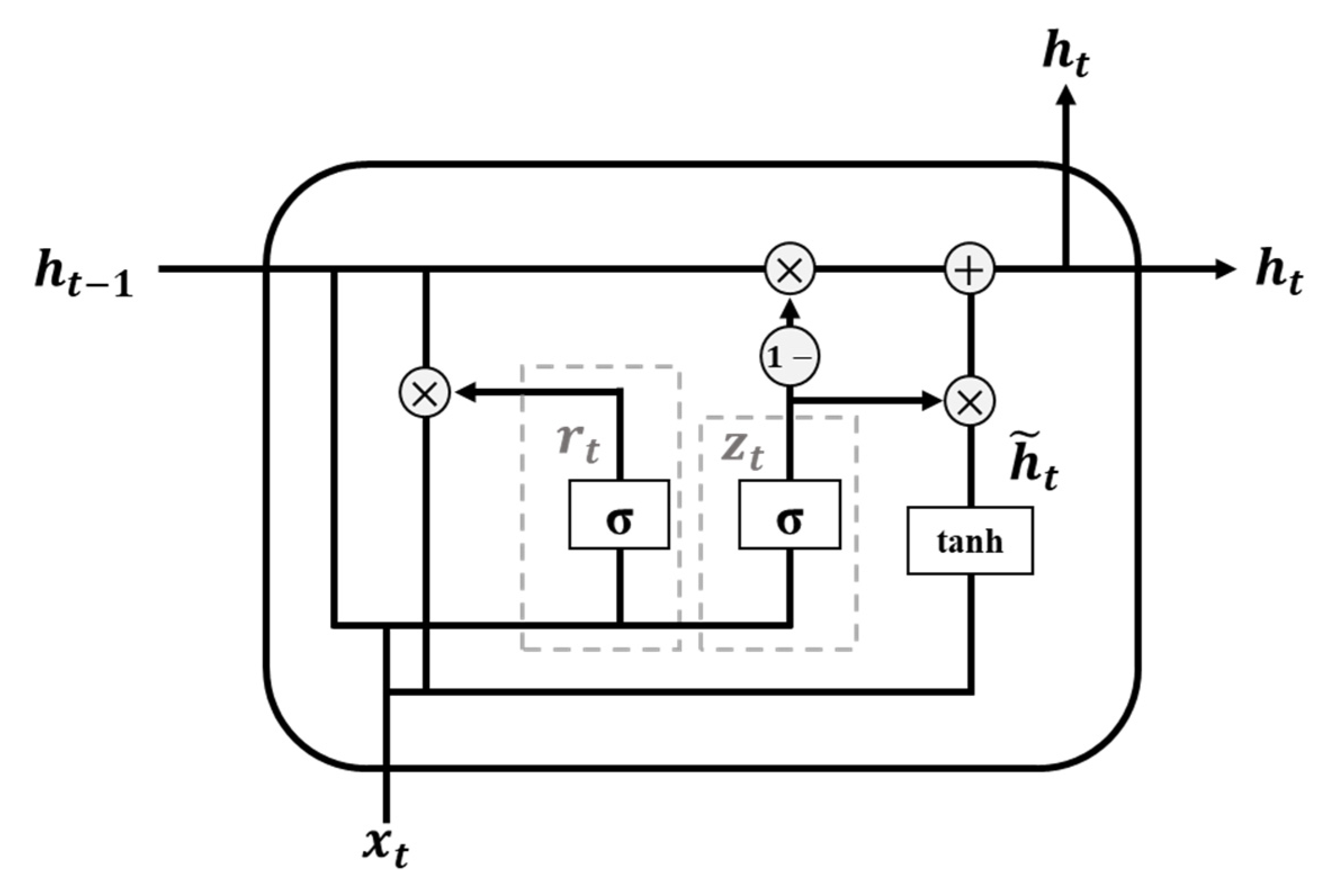
2.3.2. Gated Recurrent Unit (GRU)

The GRU is derived from LSTM with fewer parameters and higher computational efficiency. It has two gates, called update and reset gates, to control the information transferred in the hidden state. The role of the update gate is to control which parts of information can be updated or preserved in the next hidden state. The reset gate controls which parts of the previous hidden state are used to merge the new input information. The model structure of GRU is shown in Figure 3, and the mathematical steps can be shown as the following equations [17]:
z t = σ ( W z h t 1 , x t + b z )
r t = σ ( W r h t 1 , x t + b r )
h ~ t = t a n h ( W h r t h t 1 , x t + b h )
h t = 1 z t h t 1 + z t h ~ t
where z t and r t denote the vectors of the update and reset gates of the GRU units; h ~ t represents the new hidden state content; h t indicates the hidden state; x t refers to the input vector; W z , W r , and W h stand for the weight matrices; b z , b r , and b h represent the bias vectors; σ ( · ) denotes the sigmoid function; tanh ( · ) indicates the hyperbolic tangent function, and represents the element-wise product.

2.3.3. Bi-Directional LSTM (BILSTM)

The BILSTM network consists of forward and backward LSTM, which can process sequential data in the forward and backward directions. The above characteristics allow the network to capture information from past and future contexts, enhancing its ability to understand the temporal dependencies within the data. The BILSTM network structure is shown in Figure 4 and was implemented with the following equations [21]:
h t f = f ( W x f x t + W h f h t 1 f + b h f )
h t b = f ( W x b x t + W h b h t + 1 b + b h b )
y t = g ( W y f h t f + W y f h t b + b y )
where h t f denotes the output of the forward layer; h t b represents the output of the backward layer; y t indicates the network output; x t refers to the input vector; W x f , W h f , W x b , W h b , W y f , and W y f stand for the weight matrices; b h f , b h b , and b y denote the bias vectors; and f ( · ) and g ( · ) represent the nonlinear activation functions.

2.3.4. Climate Data Preprocessing and Model Hyperparameter Settings

In all, 109,780 climate data items collected from Greenhouse #1 were split into three parts for model training (90%), validation (5%), and testing (5%), respectively. There was a total of 1599 items of missing data in this dataset, and the missing data were imputed by linear interpolation. Upon the calculation of the value of the function at a known point, the approximate value of the function at other points can be estimated so that the available data can be used to estimate the missing data. Next, a Min–Max normalization process was used to make the input variables fall between 0 and 1 inclusive to ensure an equal contribution of each feature.
Nine different temperature forecasting models were tested in the study. Three types of RNN, i.e., LSTM, GRU, and BILSTM, were considered with the number of hidden layers ranging from 1 to 3 layers. The model structure and the corresponding names are presented in Table 1. The optimization of the number of hidden units was executed using grid search, with the number of hidden units set from 10 to 200 with a step size of 10. In addition to changing the number of hidden layers and neurons, other hyperparameters were fixed as follows: the number of epochs was 50 and the batch size was 32. The number of the kernel was initialized to zero. The sigmoid and hyperbolic tangent functions were used as activation functions. The type of loss function was the mean square error and the Adam algorithm was used as the optimizer. The learning rate was set to 10−4, and the momentum of the neural network models was 0.99. In addition, this study chose a 90%–5%–5% split to allow the models to learn changing patterns well, but this extreme split could bring the risk of overfitting. Therefore, L2 regularization, dropout rate, and patience value were considered to prevent overfitting. L2 regularization is a commonly used technique to prevent overfitting by penalizing the model for having a large weight, which helps the model to prevent from fitting the noise in the training data [32]. Moreover, overfitting can be reduced by using dropout procedure [33], and the conventional dropout rate is 0.2 or 0.3. In this study, a higher dropout rate (0.4) was assigned to strengthen the effect. Finally, a patience value of 5 was set so that if there was no improvement in the validation error after 5 epochs, the model training process was stopped.

2.3.5. Evaluation Metrics of Temperature Forecasting Model

The forecasting models established with Greenhouse #1 data were subsequently evaluated in Greenhouse #2 to assess the generalizability of the proposed models and reduce the possibility of overfitting. The statistical indicators used to evaluate the temperature forecasting model’s performance were the coefficient of determination (R2), mean absolute percentage error (MAPE), and root mean square error (RMSE) [34]. The corresponding equations are as follows:
R 2 = 1 S S E S S T O = 1 i = 1 N ( Y o b s , i Y m o d e l , i ) 2 i = 1 N ( Y o b s , i Y ¯ o b s , i ) 2 .
M A P E = i = 1 N Y o b s , i Y m o d e l , i Y o b s , i N × 100 %
R M S E = 1 N i = 1 N ( Y o b s , i Y m o d e l , i ) 2
where N denotes the total number of data items, S S E indicates the sum of the squared error, S S T O represents the total sum of the squares, Y o b s , i stands for the actual observations, Y m o d e l , i refers to the model output, and Y ¯ o b s , i denotes the mean value of the actual observations.
The value of R2 was between 0 and 1 inclusive, which was an indicator to evaluate the linear relationship between the predicted and the observed values. RMSE was used to measure the deviation between the predicted value and the observed value, with a value from 0 to infinity. MAPE was applied to quantify and evaluate the accuracy of the predicted value.

2.4. Sigmoid Model for Predicting Greenhouse Tomato Growth

For establishing the growth model, GDD (Equation (17)) [27] was used as the input variable; LAI, fresh fruit weight, and aboveground dry matter were utilized as the output variables. Two sigmoid models, namely the Logistic (Equation (18)) [35] and Gompertz (Equation (19)) [36], were used to fit the growth data and both require three parameters to characterize tomato growth:
G D D = i = 1 d a y T i T b a s e
where T i denotes the daily mean temperature (°C), T b a s e represents the base temperature ( T b a s e = 10   ° C in this study), and d a y indicates the days after the transplantation.
y i = β 1 1 + e β 2 β 3 x i + ε i
y i = β 1 e e β 2 β 3 x i + ε i
where β 1 denotes the asymptotic value of the dependent variable, β 2 indicates the location parameter related to the initial value of the model, β 3 represents the parameter that affects the growth rate in the curve, e refers to the base of the natural logarithm, and ε i stands for the error term.
In this study, growth models were constructed to link greenhouse temperature forecasts with tomato growth prediction using the GDD predicted from the proposed temperature forecasting model. Additionally, the percentage error (Equation (20)) was calculated to evaluate the difference in the parameter estimates between the growth models built using the predicted or the actual GDD as the input variable:
%   e r r o r = E A A × 100 %
where E and A denote the parameter estimates of the growth model, which were calculated using the predicted and the actual GDD, respectively.

2.5. Data Analysis Software

The microclimate prediction models were developed using Tensorflow2.6 based on Python (version 3.7), and the tomato growth data were analyzed using R software (version 4.0.5), with the “drc” (version 3.0-1) package [37] for the growth model fitting.

3. Results and Discussion

This study focused on utilizing various RNN structures and hidden units to identify the optimal structure for microclimate temperature forecasting in greenhouse tomato production. The goal was to integrate the improved prediction results with the sigmoid growth models to manage greenhouse tomato production. This would be capable of forecasting changes in the greenhouse temperature for the following 30 min and providing a prediction indicator for tomato growth.

3.1. Performance Evaluation of Temperature Forecasting Model

Greenhouse #1 data were divided into 90% training data, 5% validation data, and 5% testing data to allow the proposed models to learn the changing patterns. However, this scheme might be too constrictive to allow for unbiased error estimations in the independent testing set, so it was difficult to determine whether the testing performance was due to overfitting. Therefore, a total of 17,843 climate data collected from Greenhouse #2 were utilized as another testing set to evaluate the generalizability of the proposed forecasting models established using the Greenhouse #1 data and reduce the possibility of overfitting. As mentioned previously, Greenhouse #2 had different specifications (29.2 m long, 24 m wide, and 4.4 m ridge height; covered by a 0.15 mm plastic film) and tomato variety (beef tomato cv. “993”) from Greenhouse #1 (12 m long, 5 m wide, and 4.3 m ridge height; covered by a 0.18 mm plastic film and planted cherry tomato cv. “Rosada”). The boxplots also show that the distributions of external and internal climate data collected from the two greenhouses are slightly different (Figure 5). Therefore, Greenhouse #2 can be regarded as a different condition to test the forecasting models established in Greenhouse #1.
The forecasting ability of the temperature inside the greenhouse based on different forecasting models was evaluated using R2, MAPE, and RMSE, respectively. When the MAPE value is less than 10%, it indicates an accurate prediction. R2 was closer to 1, and RMSE was closer to 0, suggesting a more accurate predicted result. Figure 6 shows the R2 tendencies for the LSTM, GRU, and BILSTM models with different numbers of hidden layers and hidden units when forecasting the 30-min-ahead temperature inside Greenhouse #2. The following characteristics were observed: (1) the best accuracy in each model with the number of hidden units was not very low or high, (2) the accuracy was not always better for the three-layer-type models than that for the single-layer-type or two-layer-type models, and (3) the accuracy of the GRU had a large degree of variability.
The best performance and the corresponding number of hidden units for each temperature forecasting model are listed in Table 2. The GRU2 model with 60 hidden units and the LSTM2 model with 190 hidden units obtained better R2 values and lower MAPE and RMSE values among the nine models. With an accurate temperature forecast model, growers can make early decisions based on the forecast results to control the temperature in the greenhouse within a suitable range. Previous research has demonstrated that ANNs have significant advantages in their flexibility to adapt to nonlinear and non-physical data—this characteristic provides ANNs with considerable potential for application to the environmental control of greenhouses [38]. ANNs on greenhouse microclimate prediction, such as multilayer perceptron [7,39], radial basis function [40], and RNN based on LSTM, GRU, or BILSTM [18,19,21], have exhibited satisfactory performances on temperature prediction. Considering the performance of each model, the LSTM2 with 190 hidden units was chosen as the best temperature forecasting model and had an R2 of 0.962, MAPE of 3.2%, and RMSE of 1.2 °C (Table 2); its forecasting results were subsequently used to calculate the predicted GDD.

3.2. Comparison of Daily Mean Temperature and GDD between Predicted and Observed Values

As the calculation of GDD required the daily mean temperature, the predicted temperatures of the LSTM2 model were applied to calculate the daily mean temperature. Figure 7 presents the comparison results of the predicted daily mean temperature and the observed daily mean temperature during the period from October 2021 to January 2022 inside Greenhouse #2. During the four months of the test period, the daily mean temperatures predicted by the forecasting model were very close to the actual values. Furthermore, the fitted regression line for the predicted and the observed values almost overlapped with a straight line with a slope of 1 and its R2 was 0.981 (Figure 8). These results show that the LSTM2 model is accurate in predicting internal temperature and has no tendency of overestimation or underestimation, even when applied to a greenhouse that was not used in the modeling.
LSTM2 (the best model) and BILSTM2 (the worst model with a lower R2 and higher MAPE and RMSE) were compared to demonstrate the benefits of accurate temperature forecasting models. The GDD values were calculated using the observed and predicted mean temperatures from the two temperature forecasting models. Figure 9 shows the observed and predicted GDD values for the 94-day investigation period. For the last day of investigation, the predicted GDD calculated using the results of the LSTM2 model was 16.28 °C higher than the observed GDD. However, the predicted GDD calculated using the BILSTM2 model results was 65.47 °C higher than the observed GDD. The comparison results indicated that if the temperature forecasting model had a better performance, the value of the predicted GDD would be closer to the actual value. As the prediction error of the forecasting model increased over time, the difference between the predicted and the observed GDD values increased. When the crop growth days were longer, the gap between the actual and the predicted values would be wider. Therefore, an accurate temperature forecasting model would be beneficial for monitoring the changes in the microclimate conditions inside the greenhouse.

3.3. Sigmoid Growth Model for Greenhouse Tomato Production

Even though previous research has used deep learning models to predict greenhouse crop yields based on historical yields and greenhouse internal environment variables [41,42], the major drawback of these models is that they cannot clearly describe the relationship between input and output due to their black-box nature [43]. On the contrary, the advantage of using the sigmoid model to fit growth characteristics is that the parameters can be related to the biological meaning of the processes [25,27], which implies that researchers can apply the sigmoid model to relate the environmental condition to crop growth and development. Furthermore, the phenology model based on the GDD could be used to predict tomato growth stages and guide adaptive management decisions, particularly in response to climate or planting environment changes [44].
For the establishment of the tomato growth model, two sigmoid models, namely Logistic and Gompertz, were used to relate the three important growth traits (i.e., LAI, fresh fruit weight, and aboveground dry matter) to the GDD. Table 3 and Table 4 present the parameter estimation results obtained by fitting the Logistic and Gompertz models using the observed GDD and the LSTM2-predicted GDD values, respectively. The parameter estimation results were very close, irrespective of whether the observed or the predicted GDD values were used for the input variables. While exploring the scatter plots of the different growth traits against the GDD, it could be observed that the relationships between the three growth traits and the GDD closely resemble an S-shaped curve (Figure 10 and Figure 11). For each trait, both the Logistic and Gompertz models provided a good description of the relationship between the traits and the GDD and exhibited a similar performance, with R2 values ranging between 0.80 and 0.91. This indicated that the predicted temperature results obtained from the temperature forecasting model were highly effective in fitting the growth models and accurately predicting various important traits of tomatoes. As a common crop growth index, LAI is closely related to photosynthesis, evapotranspiration, dry matter accumulation, and the aboveground productivity of crops. The general method of measuring LAI is mainly through destructive sampling or by using canopy analyzers and spectral telemetry. These methods are time-consuming or have high instrument costs [45]. Therefore, the establishment of the LAI model is helpful to track the growth status of crops. High yield is one of the most important objects of greenhouse cultivation. With the yield prediction model, relevant information can be obtained before crop harvesting, which can be used as the base for subsequent harvesting, storage, and other planning.

3.4. Limitations of Present Study and Suggestions for Future Works

The best temperature forecasting model proposed in this study has an R2 of 0.962, MAPE of 3.2%, and RMSE of 1.2 °C, but the performance can be further improved by increasing the data collection period, or by grouping the data into different seasons to establish a model which is suitable for each season [34]. Although the proposed model has been evaluated using another different-sized plastic greenhouse, the model’s performance may be reduced when applied in different regions or climate conditions. Therefore, the generalizability of the proposed forecasting model needs to be tested in various conditions. Furthermore, to the best of our knowledge, the most suitable deep learning model for modeling time series data is the RNN and its derived models, so three types of RNN (i.e., LSTM, GRU, and BILSTM) were used to build a temperature forecasting model. However, for 30-min-ahead temperature forecasting, it is possible to achieve acceptable accuracy using simpler models; therefore, simpler models should be considered for building microclimate forecasting models to reduce training time and computing costs.
Furthermore, light, humidity, and CO2 concentrations are also important microclimate factors related to crop production and environmental control in greenhouses [19,46,47]. Therefore, forecasting models for these microclimate factors could also be developed. Finally, this study only utilized GDD as the input to simulate tomato growth. In the future, different environmental data could be considered to improve the accuracy of growth simulations for a more comprehensive greenhouse production framework.

4. Conclusions

Greenhouse production needs to consider various factors such as greenhouse type, environmental control, crop physiology, efficient resource utilization, and production costs. This study collected two-year climate data to develop a temperature forecasting model to predict the greenhouse temperature. The proposed LSTM2 model demonstrated that the temperature trends could be forecasted accurately, and the model could be used in plastic greenhouses, irrespective of the differences in the greenhouse size or tomato variety. Furthermore, the predicted temperature was used to calculate the GDD and establish different tomato growth models. Similar model parameter estimates of the tomato growth model were obtained when using the predicted GDD or the observed GDD. These findings reveal the potential of utilizing microclimate forecasting to manage greenhouse production and optimize crop production processes. When greenhouses are densely distributed in an agricultural production area, the weather stations nearby can be utilized to collect the external climate data for the greenhouses. These data can then be used to predict the microclimate changes inside the greenhouses by utilizing a temperature forecasting model. In addition, it can potentially reduce the need for expensive sensor installations and make greenhouse management more accessible and cost-effective. Furthermore, the forecasted microclimate data can be applied to predict the growth of tomatoes, and the prediction results can provide feedback to farmers or a reference for the decision-making and optimization of greenhouse production conditions.

Author Contributions

Conceptualization, Y.-S.L.; methodology, Y.-S.L.; software, Y.-S.L.; formal analysis, Y.-S.L. and S.-L.F.; investigation, S.-L.F., L.K. and C.-C.C.; resources, L.K., C.-C.C. and M.-H.Y.; data curation, S.-L.F., L.K. and C.-C.C.; writing—original draft preparation, Y.-S.L. and S.-L.F.; writing—review and editing, M.-H.Y. and B.-J.K.; visualization, Y.-S.L.; supervision, B.-J.K.; project administration, M.-H.Y. and B.-J.K.; funding acquisition, M.-H.Y. and B.-J.K. All authors have read and agreed to the published version of the manuscript.

Funding

This work was financially supported by the National Science and Technology Council (NSTC) in Taiwan (grant number NSTC 112-2621-M-005-005). This research was also supported (in part) by NSTC 112-2634-F-005-002—project Smart Sustainable New Agriculture Research Center (SMARTer).

Data Availability Statement

The original contributions presented in the study are included in the article, further inquiries can be directed to the corresponding author.

Conflicts of Interest

The authors declare no conflicts of interest.

References

  1. Li, H.; Wang, S. Technology and studies for greenhouse cooling. World J. Eng. Technol. 2015, 3, 73–77. [Google Scholar] [CrossRef]
  2. Singh, M.C.; Yousuf, A.; Singh, J.P. Greenhouse microclimate modeling under cropped conditions—A review. Res. Environ. Life Sci. 2016, 9, 1552–1557. [Google Scholar]
  3. Escamilla-Garcia, A.; Soto-Zarazúa, G.M.; Toledano-Ayala, M.; Rivas-Araiza, E.; Gastélum-Barrios, A. Applications of artificial neural networks in greenhouse technology and overview for smart agriculture development. Appl. Sci. 2020, 10, 3835. [Google Scholar] [CrossRef]
  4. Ma, D.; Carpenter, N.; Maki, H.; Rehman, T.U.; Tuinstra, M.R.; Jin, J. Greenhouse environment modeling and simulation for microclimate control. Comput. Electron. Agric. 2019, 162, 134–142. [Google Scholar] [CrossRef]
  5. Frausto, H.U.; Pieters, J.G. Modelling greenhouse temperature using system identification by means of neural networks. Neurocomputing 2004, 56, 423–428. [Google Scholar] [CrossRef]
  6. Pawlowski, A.; Guzmán, J.L.; Rodríguez, F.; Berenguel, M.; Sanchez, J.; Dormido, S. Event-based control and wireless sensor network for greenhouse diurnal temperature control: A simulated case study. In Proceedings of the 2008 IEEE International Conference on Emerging Technologies and Factory Automation (EFTA), Hamburg, Germany, 15–18 September 2008; pp. 500–507. [Google Scholar] [CrossRef]
  7. Petrakis, T.; Kavga, A.; Thomopoulos, V.; Argiriou, A.A. Neural network model for greenhouse microclimate predictions. Agriculture 2022, 12, 780. [Google Scholar] [CrossRef]
  8. Katzin, D.; van Henten, E.J.; van Mourik, S. Process-based greenhouse climate models: Genealogy, current status, and future directions. Agric. Syst. 2022, 198, 103388. [Google Scholar] [CrossRef]
  9. Ali, R.B.; Bouadila, S.; Mami, A. Experimental validation of the dynamic thermal behavior of two types of agricultural greenhouses in the Mediterranean context. Renew. Energy 2020, 147, 118–129. [Google Scholar] [CrossRef]
  10. Pawlowski, A.; Sánchez-Molina, J.A.; Guzmán, J.L.; Rodríguez, F.; Dormido, S. Evaluation of event-based irrigation system control scheme for tomato crops in greenhouses. Agric. Water Manag. 2017, 183, 16–25. [Google Scholar] [CrossRef]
  11. Wang, L.; Li, X.; Xu, M.; Guo, Z.; Wang, B. Study on optimization model control method of light and temperature coordination of greenhouse crops with benefit priority. Comput. Electron. Agric. 2023, 210, 107892. [Google Scholar] [CrossRef]
  12. Ehret, D.L.; Hill, B.D.; Helmer, T.; Edwards, D.R. Neural network modeling of greenhouse tomato yield, growth and water use from automated crop monitoring data. Comput. Electron. Agric. 2011, 79, 82–89. [Google Scholar] [CrossRef]
  13. Küçükönder, H.; Boyaci, S.; Akyüz, A. A modeling study with an artificial neural network: Developing estimation models for the tomato plant leaf area. Turk. J. Agric. For. 2016, 40, 203–212. [Google Scholar] [CrossRef]
  14. Pandey, S.K.; Janghel, R.R. Recent deep learning techniques, challenges and its applications for medical healthcare system: A review. Neural Process. Lett. 2019, 50, 1907–1935. [Google Scholar] [CrossRef]
  15. Bengio, Y.; Simard, P.; Frasconi, P. Learning long-term dependencies with gradient descent is difficult. IEEE Trans. Neural Netw. 1994, 5, 157–166. [Google Scholar] [CrossRef]
  16. Hochreiter, S.; Schmidhuber, J. Long short-term memory. Neural Comput. 1997, 9, 1735–1780. [Google Scholar] [CrossRef]
  17. Cho, K.; Van Merriënboer, B.; Gulcehre, C.; Bahdanau, D.; Bougares, F.; Schwenk, H.; Bengio, Y. Learning phrase representations using RNN encoder-decoder for statistical machine translation. arXiv 2014, arXiv:1406.1078. [Google Scholar] [CrossRef]
  18. Elhariri, E.; Taie, S.A. H-ahead multivariate microclimate forecasting system based on deep learning. In Proceedings of the 2019 International Conference on Innovative Trends in Computer Engineering (ITCE), Aswan, Egypt, 2–4 February 2019; pp. 168–173. [Google Scholar] [CrossRef]
  19. Jung, D.H.; Kim, H.S.; Jhin, C.; Kim, H.J.; Park, S.H. Time-serial analysis of deep neural network models for prediction of climatic conditions inside a greenhouse. Comput. Electron. Agric. 2020, 173, 105402. [Google Scholar] [CrossRef]
  20. Yao, M.-H.; Wang, H.-C.; Chiu, Y.-W.; Hsieh, H.-C.; Chang, T.-H.; Lee, Y.-J. Integrating microweather forecasts and crop physiological indicators for greenhouse environmental control. Acta Hortic. 2021, 1327, 445–454. [Google Scholar] [CrossRef]
  21. Hao, X.; Liu, Y.; Pei, L.; Li, W.; Du, Y. Atmospheric temperature prediction based on a BiLSTM-Attention model. Symmetry 2022, 14, 2470. [Google Scholar] [CrossRef]
  22. Vijayakumar, A.; Beena, R. Impact of temperature difference on the physicochemical properties and yield of tomato: A review. Chem. Sci. Rev. Lett. 2020, 9, 665–681. [Google Scholar]
  23. McMaster, G.S.; Wilhelm, W.W. Growing degree-days: One equation, two interpretations. Agric. For. Meteorol. 1997, 87, 291–300. [Google Scholar] [CrossRef]
  24. Cao, L.; Shi, P.J.; Li, L.; Chen, G. A new flexible sigmoidal growth model. Symmetry 2019, 11, 204. [Google Scholar] [CrossRef]
  25. Archontoulis, S.V.; Miguez, F.E. Nonlinear regression models and applications in agricultural research. Agron. J. 2015, 107, 786–798. [Google Scholar] [CrossRef]
  26. Zeide, B. Analysis of growth equations. For. Sci. 1993, 39, 594–616. [Google Scholar] [CrossRef]
  27. Fang, S.-L.; Kuo, Y.-H.; Kang, L.; Chen, C.-C.; Hsieh, C.-Y.; Yao, M.-H.; Kuo, B.-J. Using sigmoid growth models to simulate greenhouse tomato growth and development. Horticulturae 2022, 8, 1021. [Google Scholar] [CrossRef]
  28. Meade, K.A.; Cooper, M.; Beavis, W.D. Modeling biomass accumulation in maize kernels. Field Crops Res. 2013, 151, 92–100. [Google Scholar] [CrossRef]
  29. Wu, Y.; Yan, S.; Fan, J.; Zhang, F.; Xiang, Y.; Zheng, J.; Guo, J. Responses of growth, fruit yield, quality and water productivity of greenhouse tomato to deficit drip irrigation. Sci. Hortic. 2021, 275, 109710. [Google Scholar] [CrossRef]
  30. Hsieh, C.-Y.; Fang, S.-L.; Wu, Y.-F.; Chu, Y.-C.; Kuo, B.-J. Using sigmoid growth curves to establish growth models of tomato and eggplant stems suitable for grafting in subtropical countries. Horticulturae 2021, 7, 537. [Google Scholar] [CrossRef]
  31. Greff, K.; Srivastava, R.K.; Koutník, J.; Steunebrink, B.R.; Schmidhuber, J. LSTM: A search space odyssey. IEEE Trans. Neural Netw. Learn. Syst. 2016, 28, 2222–2232. [Google Scholar] [CrossRef] [PubMed]
  32. Van Laarhoven, T. L2 regularization versus batch and weight normalization. arXiv 2017, arXiv:1706.05350. [Google Scholar] [CrossRef]
  33. Hinton, G.E.; Srivastava, N.; Krizhevsky, A.; Sutskever, I.; Salakhutdinov, R.R. Improving neural networks by preventing co-adaptation of feature detectors. arXiv 2012, arXiv:1207.0580. [Google Scholar] [CrossRef]
  34. Esparza-Gómez, J.M.; Luque-Vega, L.F.; Guerrero-Osuna, H.A.; Carrasco-Navarro, R.; García-Vázquez, F.; Mata-Romero, M.E.; Olvera-Olvera, C.A.; Carlos-Mancilla, M.A.; Solís-Sánchez, L.O. Long short-term memory recurrent neural network and extreme gradient boosting algorithms applied in a greenhouse’s internal temperature prediction. Appl. Sci. 2023, 13, 12341. [Google Scholar] [CrossRef]
  35. Verhulst, P.F. A note on population growth. Corresp. Math. Phys. 1838, 10, 113–121. [Google Scholar]
  36. Gompertz, B. On the nature of the function expressive of the law of human mortality, and on a new mode of determining the value of life contingencies. Philos. Trans. R. Soc. 1825, 115, 513–585. [Google Scholar] [CrossRef]
  37. Ritz, C.; Strebig, J.C. Package ‘drc’. Title Analysis of Dose-Response Curves. 2016. Available online: https://cran.r-project.org/web/packages/drc/drc.pdf (accessed on 1 February 2024).
  38. Seginer, I. Some artificial neural network applications to greenhouse environmental control. Comput. Electron. Agric. 1997, 18, 167–186. [Google Scholar] [CrossRef]
  39. Dariouchy, A.; Aassif, E.; Lekouch, K.; Bouirden, L.; Maze, G. Prediction of the intern parameters tomato greenhouse in a semi-arid area using a time-series model of artificial neural networks. Measurement 2009, 42, 456–463. [Google Scholar] [CrossRef]
  40. Hu, H.G.; Xu, L.H.; Wei, R.H.; Zhu, B.K. RBF network based nonlinear model reference adaptive PD controller design for greenhouse climate. Int. J. Adv. Comput. Technol. 2011, 3, 357–366. [Google Scholar] [CrossRef]
  41. Cho, W.; Kim, S.; Na, M.; Na, I. Forecasting of tomato yields using attention-based LSTM network and ARMA model. Electronics 2021, 10, 1576. [Google Scholar] [CrossRef]
  42. Gong, L.; Yu, M.; Jiang, S.; Cutsuridis, V.; Pearson, S. Deep learning based prediction on greenhouse crop yield combined TCN and RNN. Sensors 2021, 21, 4537. [Google Scholar] [CrossRef]
  43. Goyal, P.; Kumar, S.; Sharda, R. A review of the Artificial Intelligence (AI) based techniques for estimating reference evapotranspiration: Current trends and future perspectives. Comput. Electron. Agric. 2023, 209, 107836. [Google Scholar] [CrossRef]
  44. Pathak, T.B.; Stoddard, C.S. Climate change effects on the processing tomato growing season in California using growing degree day model. Model. Earth Syst. Environ. 2018, 4, 765–775. [Google Scholar] [CrossRef]
  45. Martínez-Ruiz, A.; López-Cruz, I.L.; Ruiz-García, A.; Pineda-Pineda, J.; Prado-Hernández, J.V. HortSyst: A dynamic model to predict growth, nitrogen uptake, and transpiration of greenhouse tomatoes. Chil. J. Agric. Res. 2019, 79, 89–102. [Google Scholar] [CrossRef]
  46. Badji, A.; Benseddik, A.; Bensaha, H.; Boukhelifa, A.; Hasrane, I. Design, technology, and management of greenhouse: A review. J. Clean. Prod. 2022, 373, 133753. [Google Scholar] [CrossRef]
  47. Rodríguez, F.; Berenguel, M.; Guzmán, J.L.; Ramírez-arias, A. Modeling and Control of Greenhouse Crop Growth; Springer: Berlin/Heidelberg, Germany, 2014; ISBN 9783319111339. [Google Scholar]
Figure 2. Basic structure of LSTM.
Horticulturae 10 00230 g002
Figure 3. Basic structure of GRU.
Horticulturae 10 00230 g003
Figure 4. Basic structure of BILSTM.
Horticulturae 10 00230 g004
Figure 5. Box plots of the external and internal climate data of different datasets.
Horticulturae 10 00230 g005
Figure 6. R2 for LSTM, GRU, and BILSTM models with the different numbers of hidden layers and hidden units: (a) LSTM models, (b) GRU models, and (c) BILSTM models. The temperature data used for evaluation were collected from Greenhouse #2.
Horticulturae 10 00230 g006
Figure 7. Comparison between the predicted and observed daily mean temperatures for Greenhouse #2. Data were collected from October 2021 to January 2022.
Horticulturae 10 00230 g007
Figure 8. Scatter plot of LSTM2-predicted and observed internal daily mean temperatures for Greenhouse #2. The solid points (•) denote the predicted and observed daily mean temperatures. The solid line (—) represents the fitted regression line, and the dashed line (---) indicates the straight line with a slope of 1.
Horticulturae 10 00230 g008
Figure 9. Growing degree days calculated using the observed daily mean temperature and predicted daily mean temperature for Greenhouse #2.
Horticulturae 10 00230 g009
Figure 10. Scatter plots of the actual growth trait observations versus the observed growing degree days and the predicted growing degree days, respectively. The solid point (•) denotes the observed trait values and the growing degree days, and the blue curves represent the predicted value using the Logistic growth model. (a) Leaf area index, (b) fresh fruit weight, and (c) dry matter fitted with the growing degree days calculated using the observed daily mean temperature. (d) Leaf area index, (e) fresh fruit weight, and (f) dry matter fitted with the growing degree days calculated using the LSTM2-predicted daily mean temperature.
Horticulturae 10 00230 g010
Figure 11. Scatter plots of the actual growth trait observations versus the observed growing degree days and the predicted growing degree days. The solid point (•) denotes the observed trait values and the growing degree days, and the blue curves represent the predicted value obtained using the Gompertz growth model. (a) Leaf area index, (b) fresh fruit weight, and (c) dry matter fitted with the growing degree days calculated using the observed daily mean temperature. (d) Leaf area index, (e) fresh fruit weight, and (f) dry matter fitted with the growing degree days calculated using the LSTM2-predicted daily mean temperature.
Horticulturae 10 00230 g011
Table 1. Names and corresponding structures for the proposed temperature forecasting models.
Model NameStructure
LSTM1One-layer LSTM and one dense layer
LSTM2Two-layer LSTM and one dense layer
LSTM3Three-layer LSTM and one dense layer
GRU1One-layer GRU and one dense layer
GRU2Two-layer GRU and one dense layer
GRU3Three-layer GRU and one dense layer
BILSTM1One-layer BILSTM and one dense layer
BILSTM2Two-layer BILSTM and one dense layer
BILSTM3Three-layer BILSTM and one dense layer
Table 2. Best performance and number of hidden units for nine temperature forecasting models. The temperature data used for evaluation were collected from Greenhouse #2.
ModelNumber of Hidden UnitsR2MAPE (%)RMSE (°C)
LSTM11700.9613.4291.210
LSTM21900.9623.2161.196
LSTM31900.9583.4031.254
GRU1200.9613.4901.215
GRU2600.9643.2791.157
GRU31600.9583.6761.249
BILSTM11800.9603.3831.227
BILSTM21700.9543.5961.316
BILSTM31100.9583.3821.259
Table 3. Parameters of the Logistic model estimated for three growth traits. The values in parentheses represent the percentage error between two sets of model parameter estimates.
Growth TraitTemperature Data β 1 β 2 β 3
LAIObserved GDDs1.53452.96580.0039
Predicted GDDs1.52292.94870.0038
(0.76%)(0.58%)(2.56%)
Fresh fruit weightObserved GDDs1006.000013.03000.0148
Predicted GDDs1005.000012.91000.0145
(0.10%)(0.92%)(2.03%)
Dry matterObserved GDDs134.70005.32700.0064
Predicted GDDs134.70005.26500.0062
(0)(1.16%)(3.13%)
LAI: leaf area index; GDDs: growing degree days.
Table 4. Parameters of the Gompertz model determined for three growth traits. The values in parentheses represent the percentage error between two sets of model parameter estimates.
Growth TraitTemperature Data β 1 β 2 β 3
LAIObserved GDDs1.92484.11420.0020
Predicted GDDs1.89684.09180.0020
(1.45%)(0.54%)(0)
Fresh fruit weightObserved GDDs1039.00002814.00000.0095
Predicted GDDs1039.00002618.00000.0093
(0)(6.97%)(2.11%)
Dry matterObserved GDDs164.200012.79000.0032
Predicted GDDs164.700012.32000.0031
(0.30%)(3.67%)(3.13%)
LAI: leaf area index; GDDs: growing degree days.
Disclaimer/Publisher’s Note: The statements, opinions and data contained in all publications are solely those of the individual author(s) and contributor(s) and not of MDPI and/or the editor(s). MDPI and/or the editor(s) disclaim responsibility for any injury to people or property resulting from any ideas, methods, instructions or products referred to in the content.

