Review

A Review of the Main Process-Based Approaches for Modeling N2O Emissions from Agricultural Soils

by
Mara Gabbrielli
1,
Marina Allegrezza
1,*,
Giorgio Ragaglini
1,
Antonio Manco
2,
Luca Vitale
2 and
Alessia Perego
1
1
Department of Agricultural and Environmental Sciences, University of Milan, Via Celoria 2, 20133 Milan, Italy
2
Institute for Agriculture and Forest Systems in the Mediterranean (ISAFoM), P.le Enrico Fermi 1, 80055 Portici, Italy
*
Author to whom correspondence should be addressed.
Horticulturae 2024, 10(1), 98; https://doi.org/10.3390/horticulturae10010098
Submission received: 21 December 2023 / Revised: 15 January 2024 / Accepted: 17 January 2024 / Published: 19 January 2024
(This article belongs to the Special Issue Sustainable Strategies and Practices for Soil Fertility Management)

Abstract

:
Modeling approaches have emerged to address uncertainties arising from N2O emissions variability, representing a powerful methodology to investigate the two emitting processes (i.e., nitrification and denitrification) and to represent the interconnected dynamics among soil, atmosphere, and crops. This work offers an extensive overview of the widely used models simulating N2O under different cropping systems and management practices. We selected process-based models, prioritizing those with well-documented algorithms found in recently published scientific articles or having published source codes. We reviewed and compared the algorithms employed to simulate N2O emissions, adopting a unified symbol system. The selected models (APSIM, ARMOSA, CERES-EGC, CROPSYST, CoupModel, DAYCENT, DNDC, DSSAT, EPIC, SPACSYS, and STICS) were categorized by the approaches used to model nitrification and denitrification processes, discriminating between implicit or explicit consideration of the microbial pool and according to the formalization of the main environmental drivers of these processes (soil nitrogen concentration, temperature, moisture, and acidity). Models’ setting and performance assessments were also discussed. From the appraisal of these approaches, it emerged that soil chemical–physical properties and weather conditions are the main drivers of N cycling and the consequent gaseous emissions.

Graphical Abstract

1. Introduction

Commonly adopted agricultural practices aimed at improving cropping systems’ economic profitability have the potential to strongly influence, together with soil and environmental conditions, greenhouse gas (GHG) emissions, specifically those of carbon dioxide (CO2) nitrous oxide (N2O) and methane (CH4) [1]. These GHGs have the potential to impact ozone chemistry (N2O) and atmospheric oxidation status (CO2) [2]. The concern about increasing N2O emissions is related to its global warming potential, which is 265–298 times that of CO2 for a 100-year time horizon [3]. Furthermore, N2O is also considered the major stratospheric ozone-depleting substance. Agricultural practices, such as N amendment and fertilization, legume cropping, residue retention, and irrigation, tend to increase N2O production and emission above background levels and contribute to indirect reactive nitrogen volatilization and nitrate leaching [4].
Soil N2O emissions are influenced by the soil characteristics that affect primary processes that are indirectly or directly responsible for the emissions themselves: mineralization (indirectly), nitrification, and denitrification. Organic nitrogen, contained in crop residues and manure, is decomposed and mineralized by the soil microbial communities, resulting in the production of ammonium (NH4+) [5]. During nitrification, which is operated by nitrifying bacteria and involves the oxidation of ammonium to nitrate (NO3) by key enzymes (e.g., ammonia monooxygenase, hydroxylamine dehydrogenase, nitric oxide oxidase, nitrite oxidoreductase) [6], a small proportion of N is lost as N2O. In contrast, denitrification, conducted by denitrifying bacteria, involves the reduction of nitrate and nitrite to gaseous N2 and N2O [7], respectively, by nitrate and nitrite reductases [8]. Nitrification mainly occurs in well-aerated soils with moderate water content, while denitrification takes place in anaerobic conditions, mainly found in heavy soil with scarce drainage. The contribution of each process to N2O emissions is controlled and limited by soil biogeochemical characteristics (soil texture, pH, temperature, moisture, oxygen accessibility, and microbial activity), environmental conditions, and the type and amount of applied N fertilizer [9]. Finer-textured soils tend to release higher amounts of N2O compared to sandy soils [10]. This phenomenon can be attributed to the presence of predominant capillary pores in finer-textured soils, which retain water more effectively and create favorable conditions for N2O emissions from denitrification [11,12]. Soil temperature is another key element that impacts N2O emissions. An increase in soil temperature positively affects microbial growth but also reduces oxygen concentration, leading to an increase in anaerobic conditions [13,14]. Moreover, it was found that the N2/N2O ratio increased exponentially with the increasing temperature [15]. Soil acidity influences the N2/N2O ratio, too, but its effect on the nitrification and denitrification process needs further investigation [16].
Direct applications of N synthetic fertilizers increase the available pool for N cycle transformations [17]. As previous research reported [18], the time of fertilizer application influences the efficiency of fertilizer use and crop yield. When mineral fertilizer or manure is applied at rates greater than the effective crop need, N2O emission can increase because of the large pool of soil N that cannot be assimilated by the crop and remains available for the biological transformations involved in N2O production. Furthermore, N2O emissions can be enhanced due to rainfall events that increase soil moisture [19,20]. Several strategies have been developed to reduce the amount of N available for soil microorganisms, thereby decreasing nitrification and denitrification rates [21], by reducing nitrogen fertilizer inputs and applying them precisely and strategically so that nitrogen supply becomes synchronized with a specific crop demand. Also, to increase the N efficiency and delay detrimental processes, the use of urease and nitrification inhibitors is recommended [16]. This alignment minimizes the portion of N in the soil and its potential losses through volatilization of NH3, NO3 leaching, and N2O emission [22].
Quantifying N2O emissions from agricultural soils has always been challenging due to the significant spatial and temporal variations observed in this condition during field trials [23,24]. Several replications or integrations over a larger area are generally applied to capture the spatial variability at the field level, resulting from biological, chemical, and physical conditions of the soil [25]. Temporal variability in this context is assessed through several factors including measurement frequency, emission-related events timing, and the specific time of day when measurements are conducted [26,27,28].
In most research studies, direct N2O flux measurements during field trials are conducted using either manual or automated chambers in combination with a gas chromatograph or infrared analyzer [29]. These measurement techniques are conducted at relatively small spatial domains, mostly plot scales, and are suitable to capture topographic and treatment effects on N2O emissions [30]. They are cost effective and labor intensive but might effectively address the challenge of spatial variability on reported fluxes within the studied plot [31]. Automated chambers have the advantage of allowing frequent measurements of N2O soil flux since this methodology is less time consuming and dependent on human intervention. They require less data gap filling than manual chambers, which are very manpower demanding [27]. Continuous measurements of N2O fluxes at fine temporal scales (ranging from minutes to hours) are possible with the use of micrometeorological techniques [32,33] that are non-intrusive and suitable to overcome the inherent spatial variability in the process of soil N2O emission while providing reliable and accurate high-frequency measurements of turbulent fluxes of GHGs. The most adopted approach by international ecological station networks (https://fluxnet.org/, accessed on 16 November 2023) is eddy covariance [34], a well-established method relying on fast-response sonic anemometers and spectrometers. Its use is widespread at larger spatial (between 100 m and several kilometers) and temporal scales (from hours to years) [35].
The abovementioned advancements in measurement techniques have unveiled a clear diurnal pattern in N2O fluxes. This pattern, as observed in previous studies [36,37], implies that daily temperature variations and interactions between plants, soil microbial activities, and water content play significant roles in governing daily N2O fluxes. Consequently, neglecting these diurnal variations could result in errors when estimating N2O emissions. Chambers remain a valuable tool for measuring the impacts of soils, climate, and management on N2O emissions from a range of sources. However, for pragmatic reasons, observational study periods usually cover only a few years under a narrow range of conditions and are often not continuous over that time [38]. In parallel, researchers use incubation experiments to gain a deeper understanding of nitrogen dynamics [39]. During these experiments, soil samples are analyzed under controlled conditions to assess the impact of factors such as soil moisture, texture, temperature, and various fertilization treatments on gas emissions [40]. The experiments conducted under incubation offer advantages in terms of experimental control and economic viability, but they may present some limitations, as the direct measure, in representing the real conditions of soil and agricultural environment [41]. Scale and representativeness restrictions are due to the typical small-scale trial conditions and difficulty in addressing real-world variability. Furthermore, the timeframe is commonly short and, therefore, not adequate to capture long-term trends and is not suitable for ex ante assessment [42].
To address the challenge of scaling up from an agricultural field to a regional level, improve accuracy and reproducibility, and estimate N losses associated with agricultural scenarios, various estimations’ methodologies and models have been devised, spanning from straightforward regression models to fully process-based ones [43]. Commonly, the choice between one of the various estimation and modeling approaches is related to the rationale of each study and the researcher’s level of familiarity with the available models, the agricultural system involved, and data requirements and availability [44]. The IPCC Guidelines for National Greenhouse Gas Inventories proposed a simplified estimation methodology that relates estimates of direct N2O emissions from agricultural land to the quantities of nutrient N being applied [45,46]. This relation is defined by the emission factor, calculated for each type of input addition (mineral N fertilizer, organic manure, crop residue, and others) [46].
The models can either be empirical, derived from observed statistical or mathematical relationships, or process-based, developed to emulate the underlying process mechanisms [38]. Models of both types are also suitable to test hypotheses regarding biogeochemical process drivers and can be used to analyze the results of laboratory and field experiments [11]. While empirical approaches are limited to summarizing experimental data, process-based models mathematically represent one or several processes characterizing the functioning of well-delimited biological systems of fundamental or economic interest [47].
Process-based dynamic models simulate, at fine spatial and temporal scales, N2O emissions by explicitly modeling the underlying biogeochemical processes that produce N2O in soils and ecosystems, as influenced by pedoclimatic conditions and management practices. Data demand, which represents a common limitation [48,49], includes inputs such as soil properties, meteorological data, and cropping systems management practices, in addition to experimental observations required for model calibration and evaluation. Also, they often need site-specific information for accurate modeling [50,51,52]. The main advantage of using detailed input is the possibility of simulating daily soil conditions (soil temperature, soil water content, bulk density) and daily crop management (sowing and harvest, fertilization, irrigation, tillage). Indeed, process-based models’ time step is frequently 1 day, sometimes 1 h for submodels, which is appropriate to overcome the biogeochemical variation of agricultural systems that directly influence, as we reported above, the nitrification and denitrification processes. Another advantage of using detailed input data is the possibility of dividing the soil into discrete layers to describe management operations more finely (depth of soil tillage operation, fertilizer application, and crop residue burial). When differences in results arise from the application of simulation models, they can frequently be attributed to a lack of input data, to input data uncertainty, or to the inadequate resolution of biogeochemical processes. In these situations, model improvements in terms of algorithms and structure are recommended.
The aim of this work is to review and compare N2O simulation approaches, with a major focus on dynamic process-based simulation models that provide a whole cropping system representation. A recently published and comprehensive review providing insights on the algorithms employed in the simulation of the N fluxes, particularly N2O, is lacking. This work focuses on algorithm details reported for the selected models with a unified symbol system and is aimed at facilitating modeling approach comparisons and supporting algorithm implementation for further practical applications. In previous studies [53,54,55], process-based simulation approaches were successfully reviewed with, respectively, a major focus on model application scale (laboratory, field, and regional scale); model structure, strengths, and weaknesses; and emissions drivers representation (in three selected models). Comparing enforced algorithms for nitrification, denitrification, and GHG emissions provides an insightful tool for the analysis of the biogeochemical interactions concurring with N2O emissions, thus allowing the evaluation of cropping system management practices’ impacts on these processes. A comparative overview of the performances of the selected models, based on common evaluation criteria as reported by authors, is also provided.

2. Materials and Methods

2.1. Literature Search Details

The objective of the present literature search was to review the main available modeling approaches for N2O emissions simulation. Since only process-based models offer a detailed mechanistic understanding of the underlying processes responsible for N2O emissions, the study remained focused on this type of approach while the other modeling methodologies are summarized in the Supplementary Materials. We constrained the study to the process-based models simulating nitrous oxide emissions in a cropping system environment, where such losses are of particular concern. The analysis was restricted to process-based models for which detailed documentation of algorithms was available, preferably in recently published scientific articles or in published source codes. Models who took part in international model comparison exercises or model ensemble projects were also preferred. The selection of the models was carried out based on (i) the availability of recently published and highly cited/used materials and (ii) the inclusion of the mathematical description/algorithms/mathematical functions of the system processes considered in each model for simulating N2O. Among the process-based models emerging from the literature analysis, we specifically looked for those explicitly considering both nitrification and denitrification as contributors to N2O emissions.
For each model, we reported the mathematical equations used to describe the key physiological process involved in N2O emissions simulation. Concurrently, we also reviewed published materials relative to models’ application and evaluation for cropping system N2O emissions simulation performance.
The literature search was conducted both on Scopus and Web of Science databases through the implementation of the following query:
(TITLE-ABS-KEY (model OR modeling OR simulate OR simulating OR simulation OR estimation OR estimate OR approach) AND ALL (N2O OR nitrous AND oxide OR greenhouse AND gasses OR emission) AND TITLE-ABS-KEY (crop OR cropland AND soil OR agricultural AND environment) AND TITLE-ABS-KEY (flux OR fluxes OR emission)
As a result, we collected 439 papers on Scopus and 947 papers on the Web of Science. Another specific query has also been settled to identify scientific works where each model has been assessed considering its capability to simulate N2O emissions in comparison to experimentally observed data. For this purpose, we added the terms (calibrate OR validation OR evaluation OR assessment) to the first query, and we obtained 134 papers in Scopus and 281 in Web of Science. From the results of both queries, redundant titles were removed, the topic was restricted to a model with a field scale approach and a daily timestep, and the abovementioned criteria were applied. Consequently, we selected 57 papers.

2.2. Overview of the Selected Models

The following process-based models (Table 1) were the result of the abovementioned selection activity. ARMOSA—Analysis of cRopping systems for Management Optimization and Sustainable Agriculture [56], APSIM—The Agricultural Production Systems sIMulator [57], CERES-EGC—Crop Environment REsource Synthesis—Environnement et Grandes Cultures [58], CROPSYST—Cropping Systems simulation model [59], and STICS—Simulateur mulTIdisciplinaire pour les Cultures Standard [60] are five dynamic models whose primary purpose is to operate as analytical tools aimed at the impact evaluation of cropping system management on both crop production and environment. They are able to simulate a range of critical processes such as crop growth, soil C and N dynamics, and soil and water management, including nitrogen transformation like net mineralization, nitrification, and denitrification processes.
DSSAT—Decision Support System For Agrotechnology Transfer [61] has been designed to address several application contexts such as genetic modeling, on-farm and precision management, and regional environmental assessments; thus, it supports a range of utilities comprising weather, soil, and genetics tools.
EPIC—Environmental Policy Integrated Climate model [62] is an agricultural dynamic model primarily developed to address the effect of soil erosion on crop productivity.
DNDC—DeNitrification-DeComposition [52,63] and DAYCENT—DAYly CENTury [64] are specially designed to simulate nitrogen and carbon fluxes, considering soil, crop, and water dynamics. CoupModel—Coupled heat and mass transfer model for soil–plant–atmosphere systems [65] was also designed to simulate water and heat fluxes; it has later adopted high-level submodules of nitrification, denitrification, and gas transport from DNDC [52]. Both feature a detailed microbial approach to trace gas emissions forms (e.g., N2O, NO, N2, NH3, CH4, and CO2).
SPACSYS [66] is a process-based model simulating water, C, and N cycling between plants, soils, and microbes. It has been widely used to assess the impact of climate change tillage, fertilizer application, and different cultivars on agricultural systems in terms of crop yields, C and N budgets, soil physical properties, and soil water redistribution.
Table 1. Reviewed model overview. Nitrification simulation (Nit), denitrification simulation (Denit), microbial biomass explicit simulation, environmental factors considered: soil temperature (f(T)), soil moisture (f(W)), soil acidity (f(pH)), and substrate (other than ammonium and nitrate) concentration effect (f(substrate)).
ReferenceAuthorYearModelNitDenitMicrobial
Biomass
f(T)f(W)f(pH)f(substrate)
[67]Thorburn et al.2010APSIMyesyesnoyesyesonly for Nitactive carbon only for Denit
[56]Perego et al.2013ARMOSAyesyesnoyesyesonly for Nit-
[58]Gabrielle et al.2005CERES-EGCyesyesnoyesyesno-
[68]Jansson and Karlberg2010CoupModelyesyesoptional for both Nit and DenityesyesyesDOC for Nit in the microbial
explicit approach
[69]Stockle et al.2012CROPSYSTyesyesonly for SOC mineralizationonly for Nityesonly for NitCO2 for Denit
[11]Parton et al.2001DAYCENTyesyesnoonly for Nityesonly for NitCO2 for Denit
[52]Li2000DNDCyesyesyesyesonly for Nityes (indirectly for Nit)indirectly DOC for both
[70]Hoogenboom et al.2019DSSATyesyesnoonly for CERES-Denit and Nityesonly for NitCO2 for DAYCENT-Denit,
water-extractable C for
CERES-Denit
[62]Sharpley and Williams1990EPICyesyesnoyesyesonly for NitCO2 for Denit (Kemanian option)
[71]Wu et al.2015SPACSYSyesyesoptional for both Nit and Denityesonly for NityesDOC for Nit and Denit
[60]Brisson et al.2008STICSyesyesnoyesyesonly for Nit-

2.3. Statistical Indices for Model Evaluation

When reporting the application areas of the selected models, the evaluation criteria used by the authors and published in the articles were also included in this review. These evaluation indices were derived from experiments conducted for model validation and/or calibration. Typical statistical indices (Appendix A.1, Appendix A) for performance evaluations in modeling applications include Pearson’s correlation coefficient (r), coefficient of determination (R2), root mean squared error (RMSE), relative root mean squared error (RRMSE), and modeling efficiency (EF). These metrics describe the error associated with model estimates (RMSE), the total variation in observations captured by simulated data (R2), and whether the model outperforms a mean observation in the prediction of observed data (EF). When present, the other indexes have also been organized and reported in Appendix A (Appendix A.3, Table A9).

3. Results

These sections report the main approaches for nitrous oxide simulation, with a major focus on process-based models. The other concurrent alternative approaches for the prediction and estimate of soil N2O releases—such as IPCC approaches, statistical models, meta-models, and whole farm models—are reported in the Supplementary Material.

3.1. Process-Based Models

All the processes described are simulated for selected discrete soil layers at each time step unless otherwise specified. All the state and auxiliary variable values employed in the formulas correspond to the current time step value unless otherwise specified. In the following paragraphs, parameters are presented with their definition, symbol, unit of measure, and default value (when available). In this review, all variables and parameters are associated with a common symbol for all the models. The model-specific original symbols of variables (Appendix A.3, Table A1, Table A3, Table A5 and Table A7) and parameters (Appendix A.3, Table A2, Table A4, Table A6 and Table A8) are reported in Appendix A.

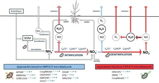
3.1.1. Nitrification

Approaches Based on Implicit Microbial Pools

In APSIM [67], the potential nitrification rate (Rnit, mg N g−1 soil d−1, Equation (1)) follows a Michaelis–Menten kinetics [72] and employs two parameters: the maximum reaction velocity (Vmax, mg N g−1 soil d−1, 40), and the ammonium concentration ([NH4]) to obtain half of Vmax (Km, mg N g−1 soil, 90). The nitrification rate is obtained by limiting the potential rate with the response function to soil acidity, soil moisture, and temperature.
R n i t = V m a x · [ N H 4 ] K m + [ N H 4 ] · min [ f T ,   f W ,   f p H ]
In the ARMOSA [56] and CROPSYST [69,73] models, the nitrification rate (Rnit, kg N ha−1 d−1, Equation (2)) is simulated using the SOILN approach [74,75]. A daily nitrification coefficient (knit, d−1, 0.2) is employed, together with the nitrate–ammonium ratio for nitrification (rNO3/NH4, unitless, 8, from 1 to 15 in agricultural soils). ARMOSA also employs a multiplicative aerobic factor (fn(OX), unitless) that simulates the effect of tillage operations within 45 days of the first application. After this period, or if meanwhile 100 mm of rain has fallen, the factor is no longer considered in the rate estimate.
R n i t = k n i t · N N H 4 N N O 3 r N O 3 / N H 4 · f n ( T ) · f n ( W )   · f n ( p H )
In CERES-EGC [76], the nitrification rate (Rnit, kg N ha−1 d−1, Equation (3)) is obtained by limiting the maximum nitrification rate (knit, kg N ha−1 d−1), representing the site-specific nitrification rate at 20 °C, with three unitless response functions to soil ammonium concentration, water-filled pore space, and temperature.
R n i t = k n i t · f n ( T ) · f n ( W ) · f n ( N H 4 )
In CoupModel [68], the nitrification rate (Rnit, g N m−2 d−1, Equation (4)) can be estimated with a simplified approach or with an explicit microbial biomass approach (Equation (10)). In the simplified approach, the nitrification rate (Rnit, g N m−2 d−1) depends on a soil acidity coefficient (kpH, unitless, 1), which is limited by the response functions to soil temperature, water-filled pore space, ammonium, and nitrate concentrations.
R n i t = f T · f n W · f n N H 4 , N O 3 · k p H
In DAYCENT [11] version 4.7, the nitrification rate (Rnit, g N m−2 d−1, Equation (5)) consists of a fraction of the daily net mineralization from the SOM submodel (Netmm, g N m−2), which is assumed to be nitrified each day (Knit2, d−1, 0.2), and in a maximum nitrified fraction (Knit, d−1, 0.1) of the soil ammonium concentration (NH4, g N m−2).
R n i t = N e t m m · k n i t 2 + k n i t · N H 4 · f n ( T ) · f n ( W ) · f n ( p H )
In DSSAT [70] V4.8.2.0 [77], the nitrification rate (Rnit, kg N ha−1 d−1, Equation (6)) is limited through response functions to soil temperature, moisture, and acidity, which range between 0 and 1, and it is further reduced in the presence of a nitrification inhibitor compound.
R n i t = N H 4 · f n 1 T · f n W + f n p H + f n 2 T
In EPIC [62] version 1102 [78], the nitrification rate (Rnit, kg N ha−1 d−1, Equation (7)) is simulated as depending on the ammonium availability, net of nitrogen volatilization (Rvol, kg N ha−1 d−1). The response function of nitrification to soil moisture is based on soil water content (f1(W)), and it is also employed in the denitrification estimate. The auxiliary variable (AKAV, unitless) estimate depends on the considered layer: for the first layer, it depends on soil temperature and wind speed; for the deeper layers, it depends on temperature and a cationic exchange capacity factor. The parameter employed (knit3, unitless, between 0 and 1) represents the upper limit of nitrification—volatilization as a fraction of the present ammonium.
R n i t = m i n k n i t 3 ,   1 e A K A V + f n ( T ) · f 1 ( W ) · f n ( p H ) · N H 4 R v o l
In the SPACSYS model [66], the nitrification rate (Rnit, g N m−2 d−1, Equation (8)) in the implicit microbial biomass approach depends on the maximum rate of nitrification (knit, d−1) parameters, which is limited by the response functions to soil temperature, water-filled pore space, and ammonium and nitrate concentration.
R n i t = k n i t · f T · f n W · f n N H 4 , N O 3
In STICS [60], nitrification occurs only in the biologically active soil layer, which is constrained by a maximum depth parameter (znit, cm, 30). The nitrification rate in each layer (Rnit, kg N ha−1 cm−1, Equation (9)) depends on the daily maximum fraction of ammonium converted in nitrate (knit, d−1) and on the ratio between N2O emissions and total nitrification (rN2O/nit, unitless). The total nitrification is obtained as the sum of each layer’s nitrification rate above the maximum depth.
R n i t = 1 r N 2 O / n i t   · k n i t · N H 4 · f n T · f n W · f n p H

Approaches Based on Explicit Microbial Pools

In CoupModel [68], when nitrifying microbials are explicitly taken into account, the nitrification rate (Rnit, g N m−2 d−1, Equation (10)) is directly proportional to a rate coefficient (knit, mg ha d−1 kg−1, 0.25) and to the nitrifiers microbial biomass (Bnit, g m−2), limited by the response functions to environmental factors and to ammonium solute concentration.
R n i t = k n i t · f T · f n W · f n N H 4 · k p H · B n i t
In DNDC model version 9.5 [79], the nitrification rate (Rnit, kg N ha−1 d−1, Equation (11)) is calculated on the base of a nitrification coefficient (knit, d−1, 0.005), the ammonium amount (kg N ha−1), the soil acidity (pH, unitless), and the nitrifiers biomass (Bnit, kg C ha−1).
R n i t = k n i t · N H 4 · B n i t · p H
For the explicit microbial pools approach of the SPACSYS model [71], the nitrification rate (Rnit, g N m−2 d−1, Equation (12)) depends on the nitrifier biomass (Bnit, g C m−2) and on the maximum rate of nitrification (knit, d−1, 0.004) parameters, which is limited by the response functions to soil temperature, water-filled pore space, soil acidity, and ammonium concentration.
R n i t = k n i t · f T · f W · f n p H · f n N H 4 · B n i t

3.1.2. Denitrification

Approaches Based on Implicit Microbial Pools

In the APSIM model [67], the denitrification rate (Rdenit, kg N ha−1 d−1, Equation (13)) is simulated as a fraction (kdenit, unitless, 0.0006) of the nitrate (kg N ha−1) amount, limited by active carbon concentration ([CA], ppm, Appendix A.2, Appendix A) and soil temperature moisture response functions.
R d e n i t = k d e n i t · N O 3 · C A · f d T · f d W  
In ARMOSA [56], the denitrification rate (Rdenit, kg N ha−1 d−1, Equation (14)) is simulated using SOILN approach [75]: a daily denitrification rate (kdenit, kg N ha−1 d−1, 0.04, between 0.04 and 0.2) is employed, together with a denitrification half-saturation constant (Km, mg N L−1, 10, between 5 and 15) defining the nitrate concentration ([NO3], kg N L−1) at which denitrification activity is half of the activity at optimum nitrate concentration.
R d e n i t = k d e n i t · N O 3 N O 3 + K m 10 6 · f ( T ) · f d ( W )
In CERES-EGC [76], the denitrification rate (Rdenit, kg N ha−1 d−1, Equation (15)) is obtained by limiting the potential rate (kdenit, kg N ha−1 d−1), representing the site-specific denitrification rate at 20 °C, with three unitless response functions to soil nitrate concentration, water-filled pore space, and temperature.
R d e n i t = k d e n i t · f d ( T ) · f d ( W ) · f d ( N O 3 )
In CoupModel [68], the denitrification rate (Rdenit, g N m−2 d−1) is either not accounted for (denitrification not simulated), or it can be calculated with a simplified approach (where the rate depends on response functions for soil temperature, soil moisture, and nitrate concentration in the soil with denitrifying microorganisms not explicitly simulated, Equation (16)) or with an explicit denitrifying microorganisms biomass approach (Equation (25)). The denitrification rate, when simulated, can be differentiated through the soil profile: it can be evenly distributed (constant), or it can decrease linearly or exponentially with the depth of the soil layer (∆z). A factor (zadj, unitless) adjusts the potential denitrification rate parameter (kdenit, g N m−2 d−1, 0.04) for each soil layer.
R d e n i t = k d e n i t · f T · f d W · f d N O 3 · z a d j ( z )
In the CROPSYST model [59,69,73], the actual denitrification rate (Rdenit, kg N ha−1 d−1, Equation (17)) is obtained by limiting a potential denitrification rate (kdenit, kg N ha−1 d−1) with environmental factors response functions [80] to soil nitrate, soil heterotrophic respiration, and water content.
R d e n i t = k d e n i t · m i n f d N O 3 , f d C O 2 · f d ( W )  
In DAYCENT model 4.7 [11], the total N flux (Rdenit, µg N g soil−1 d−1, Equation (18)) from denitrification [81] is obtained using a response function to nitrate level (fd(NO3), µg N g soil−1 d−1) and a response function to heterotrophic respiration (fd(CO2), µg N g soil−1 d−1), which surrogates labile C availability, together with a response function to WFPS (fd(W), unitless), which surrogates O2 soil status.
R d e n i t = m i n f d N O 3 , f d C O 2 · f d W
In DSSAT model [70] V4.8.2.0 [77], the denitrification of NO3 to N2O and N2 gases can be simulated using the DAYCENT or CERES denitrification subroutine. In the DAYCENT subroutine, the NO3 denitrification rate (Rdenit, kg N ha−1 d−1, Equation (19)) is derived from the DAYCENT model [81]. The denitrification rate is calculated for each soil layer and is accelerated for the soil layer whose depth (z, m) comprises 0 and the parameter zdenit (m, 0.3 default).
R d e n i t = f d W · min f d N O 3 , f d C O 2                                                   i f   z > z d e n i t f d W · m a x min f d N O 3 , f d C O 2 ,   0.066   i f   z < z d e n i t
In the CERES denitrification subroutine, denitrification only occurs when nitrate is present (NO3 > 0.01 kg N ha−1), the soil water content (SWC, m3 m−3) is higher than the drained upper limit (DUL, m3 m−3), and the soil temperature (T, K) is higher than 5. The denitrification rate (Rdenit, kg N ha−1 d−1, Equation (20)) depends on a denitrification coefficient (kdenit, d−1, 0.0006), water-extractable soil carbon (CW), nitrate content, and water and temperature response functions.
R d e n i t = k d e n i t · N O 3 · C W · f d ( W ) · f d ( T )
In EPIC model v. 1102 [62], three methods for the denitrification routine can be selected from the control file: IMWJ [82], Armen Kemanian denitrification method, and the original EPIC denitrification method [78]. The IMWJ (Izaurralde, McGill, Williams, and Jones) denitrification option (not reported) calculates the total number of electrons released by C oxidation and accepted by O2 and oxides of N (NO3, NO2 and N2O) during an hour for a given layer. The movement of N2O through the soil profile and of N2O and N2 through the liquid phase are also simulated. In the Armen Kemanian denitrification method, the denitrification rate (Rdenit, kg N ha−1 d−1, Equation (21)) is estimated by considering a parameter (kdenit, unitless, 32), the soil layer weight (WT), and the response functions to nitrate content, soil moisture, and respiration level.
R d e n i t = f d ( N O 3 ) ·   f d ( W ) · f d ( C O 2 ) ·   k d e n i t · W T · 10 3
In the original EPIC denitrification method, the denitrification rate (Rdenit, kg N ha−1 d−1, Equation (22)) employs a soil temperature factor, and two soil moisture factors (f1(W), also employed in the nitrification subroutine, and fd(W) also employed in Equation (21)).
R d e n i t = N O 3 · f d T · f 1 W · f d ( W )
In the implicit microbial biomass approach of the SPACSYS model [66], the denitrification rate (Rdenit, g N m−2 d−1, Equation (23)) depends on the maximum rate of denitrification (kdenit, g N m−2 d−1) parameter, which is limited by the response functions to soil temperature, water-filled pore space, and nitrate concentration.
R d e n i t = k d e n i t · f T · f d W · f d N O 3
In the STICS model [60], the daily denitrification rate (Rdenit, kg N ha−1 d−1, Equation (24)) is simulated with the approach of [83] only for a denitrifying soil layer (zdenit, cm, 20). A potential denitrification rate (kdenit, kg N ha−1 d−1, 16) is limited by the nitrate content, soil temperature, and moisture response functions.
R d e n i t = k d e n i t z d e n i t · f d ( T ) · f d ( N O 3 ) · f d ( W )  

Approaches Based on Explicit Microbial Pools

In CoupModel [68], when denitrifying microbes are explicitly considered, the denitrification rate is a function of their biomass (Bdenit, g C m−2) and of their activity (Mactivity, g C m−2). In this approach, NO3 concentration is obtained by dividing the nitrate amount of the zth layer for the soil water content of the layer, while NO2, NO, and N2O concentrations (NAnNxOyConc, Appendix A) are estimated by also considering the volumetric anaerobic fraction of the layer (fAnvol, auxiliary variable). These concentrations and the corresponding amount (NAnNxOy) in the considered soil layers are employed to define the total denitrification rate (Rdenit, g N m−2 d−1, Equation (25)), as the sum of the nitrogen fluxes (NAnNO2AnNO, NAnNOAnN2O and NAnN2OAnN2, i.e., out fluxes from anaerobic N pools due to microbial growth and respiration, that consumes all N from all the nitrogen anaerobic pools except for N2) of the denitrification processes steps. The nitrogen content in the anaerobic NO3 pool, i.e., soil nitrate (AnNO3, g N m−2), is employed. The equation structure describing the flux between NNO3 and AnNO2 is also used for estimating the fluxes between AnNO2 and AnNO and between AnNO and AnN2O. The equation for growth respiration (Nrg) and maintenance respiration (Nrm) are reported in Appendix A (Appendix A.2).
R d e n i t = N A n N O 2 A n N O + N A n N O A n N 2 O + N A n N 2 O A n N 2 N N O 3 A n N O 2   = m i n A n N O 3 ,   ( N r g N O 3 + N r m N O 3 ) · M a c t i v i t y · B d e n i t N A n N O 2 A n N O = m i n A n N O 2 ,   ( N r g N O 2 + N r m N O 2 ) · M a c t i v i t y · B d e n i t N A n N O A N 2 O   = m i n A n N O ,   ( N r g N O + N r m N O ) · M a c t i v i t y · B d e n i t N A n N 2 O A n N 2 = m i n A n N 2 O ,   ( N r g N 2 O + N r m N 2 O ) · f d ( N O 3 )   · M a c t i v i t y · B d e n i t
In DNDC model version 9.5 [79], the consumption rate of NxOy through denitrification (Rc,NxOy, kg N ha−1 d−1, Equation (26)) depends on the growth rate of each denitrifier group (uNxOy), the denitrifiers maximum growth yield on the corresponding substrate (YNxOy, kg C kg N−1), the maintenance coefficient on the corresponding substrate (MNxOy, kg N kg−1 h−1), the denitrifier biomass (Bdenit, kg N ha−1), the total N oxides amount (sum of NO3, NO2, NO, and N2O; ∑NxOy, kg N ha−1). Furthermore, in the DNDC model, the soil aeration status intended as a redox potential (oxygen or other oxidants content in the soil profile) is simulated. Then, the soil in each layer is divided into aerobic and anaerobic parts where nitrification and denitrification occur, respectively. When the anaerobic parts increase, more substrates (DOC, ammonium, and N oxides) are allocated to the anaerobic microsites to intensify denitrification. When the anaerobic parts decrease, nitrification will be increased due to the reallocation of the substrates into the aerobic microsites.
R c , N x O y = u N x O y Y N x O y + M N x O y · N x O y N x O y · B d e n i t · f d , N x O y p H · f d ( T )
In the explicit microbial biomass approach of the SPACSYS model [71], the consumption rate (Rc,NxOy, kg N m−3 d−1, Equation (26)) of each N oxide (NO3, NO2, NO, N2O) depends on two parameters: the maintenance coefficient on each N oxides (MNxOy; g C g−1 N d−1, Table A8), and the maximum growth yield on each N oxides (YNxOy, g C g−1 N, Table A8). The concentration of each N oxides ([NxOy], kg N m−3) and of all N oxides (∑[NxOy], kg N m−3), together with the growth rate of the NxOy denitrifiers (Rg,NxOy, kg C m−3 d−1) and their total biomass (Bdenit, g C m−2) are used. The difference from the DNDC model consists in the use of the same soil temperature response function structures for both nitrification and denitrification.

3.1.3. Emissions

In APSIM [67], ARMOSA [56], DAYCENT [11] version 4.7, DNDC version 9.5 [79], and DSSAT model [70] V4.8.2.0 [77], the N2O emissions rate during nitrification (N2Onit, kg N ha−1 d−1, Equation (27)) is estimated as a fraction (rN2O/nit, unitless, Table A6) of the nitrified N (Rnit, kg N ha−1 d−1).
N 2 O n i t = r N 2 O / n i t · R n i t
In the APSIM model, N2O emissions during denitrification (N2Odenit, kg N ha−1 d−1, Equation (28)) are obtained using the N2/N2O ratio reported by [81], the heterotrophic CO2 respiration rate (CO2,resp, µg C g soil−1 d−1), the WFPS and a parameter related to gas diffusivity in the soil at field capacity (gdiff, unitless, 25.1). The soil nitrate concentration considered is the one on a dry weight basis ([NO3], µg N g−1). In the ARMOSA model, N2O emissions due to denitrification (N2Odenit, kg N ha−1 d−1) are also simulated with a modified APSIM approach by applying the N2/N2O ratio to the denitrification rate. In Equation (28), the ratio between soil water content (SWC, m3 m−3) and saturation soil water content (SWCsat, m3 m−3) substitutes the WFPS.
N 2 N 2 O d e n i t = m a x 0.16 · g d i f f ,       k 1 · e 0.8 · [ N O 3 ] C O 2 , r e s p · m a x 0.1 ,   1.5 · W F P S 0.32
In CERES-EGC [76], N2O emissions (kg N ha−1 d−1, Equation (29)) from both nitrification and denitrification are simulated by employing site-specific parameters representing the fraction of denitrified N (rN2O/denit, unitless) and of nitrified N (rN2O/nit, unitless) emitted as nitrous dioxide.
N 2 O = r N 2 O / n i t · R n i t + r N 2 O / d e n i t · R d e n i t
In CoupModel [68], N2O and NO emissions (N2Onit and NOnit, Equation (30)) from nitrification can be simulated using the simplified approach or the microbial biomass explicit one for nitrification rate simulation, while the emissions deriving from denitrification require the explicit simulation of the denitrifiers microbial biomass. NO and N2O emissions from denitrification depend on the nitrification rate (Rnit), the maximum NO (rNO/nit, unitless, 0.004) or N2O (rN2O/nit, unitless, 0.0006) fraction parameters, and on the value of the response function for soil moisture, temperature, and acidity (Equations (45), (74), and (77)). The gaseous N forms can be emitted directly into the atmosphere from the layer in which they were formed, or the transportation of the gases through the soil profile can be simulated explicitly. Emissions from denitrification, when transportation of the gases through the soil profile is not considered, correspond to the nitrogen fluxes (NNO2AnNO, NAnNOAnN2O, NAnN2OAnN2, Equation (25)) estimated for each pool.
N 2 O n i t = r N 2 O / n i t · f e ( W ) · f e ( T ) · R n i t N O n i t   = r N O / n i t · f e ( W ) · f e ( T ) · f e ( p H ) · R n i t
In the CROPSYST model [59,69,73], N2O emissions (µg N kg−1 d−1) deriving from nitrification are modeled as a fraction of the nitrification rate (µg N kg−1 d−1), obtained through a function of soil moisture and temperature [15].
N2O emissions from denitrification (N2Odenit, µg N kg−1 d−1, Equation (31)) are modeled based on concepts and data from [81] through the application of a N2/N2O ratio (RN2/N2O, unitless, Equation (31)), which is dependent on soil nitrate (fe(NO3), unitless, Equation (99)), heterotrophic respiration (fe(CO2), unitless, Equation (100)), and water content (fe(W), unitless, Equation (72)) response functions, derived from [80].
N2 emissions from denitrification are obtained by dividing the denitrification rate by the inverse of the N2/N2O ratio plus one.
N 2 O d e n i t = R d e n i t 1 + R N 2 / N 2 O R N 2 / N 2 O = m i n f e N O 3 , f e C O 2   · f e W
In DAYCENT model [11] version 4.7, N2O emissions from denitrification are simulated with the approach of [81]. In Equation (32), fe(NO3/CO2) is a unitless function, constrained between 0 and 1, of soil gas diffusivity at field capacity (gdiff, unitless), and fe(W) is a disturbance-specific multiplier (unitless, not limited to 1, Equation (73)) that considers the effect of soil moisture (WFPS, unitless) on N2/N2O ratio (the ratio is obtained by multiplying the two functions).
N 2 O d e n i t = R d e n i t 1 + f e N O 3 C O 2 · f e ( W )
The NOx,nit+denit (g N ha−1 d−1, Equation (33)) emissions from soils are estimated on the base of the simulated N2O emission flux (N2Odenit and N2Onit) by means of a NOx/N2O ratio (RNOx/N2O, unitless, Equation (33)) and of a pulse multiplier (P, unitless) that is employed to take into account pulses in NOx emissions due to precipitation events.
N O x ,   n i t + d e n i t = R N O x / N 2 O ·   N 2 O d e n i t + R N O x / N 2 O · N 2 O n i t · P R N O x / N 2 O = 15.2 + 35.5 · a t a n 0.68 · π · 10 · g d i f f 1.86 π
In DNDC model version 9.5 [79], NO and N2O produced in either nitrification or denitrification are subject to further transformation during their diffusion through the soil matrix. The emitted fractions of the total N2O and of the total N2 evolved in a day from denitrification (P(N2O) and P(N2), unitless, Equation (34)), depending on the air-filled fraction of the total porosity (1-WFPS, unitless) and on an adsorption factor depending on clay content in the soil (fe(AD), unitless, [0–2]). In the SPACSYS model [71], the emissions rates are derived from the DNDC approach [63].
P N 2 O = 0.0006 + 0.0013 · f e ( A D ) + 0.013 0.005 · f e ( A D ) · 1 W F P S P N 2 = 0.017 + 0.025 0.0013 · f e ( A D ) · 1 W F P S
In the GHG module of DSSAT [70] V4.8.2.0 [77], the N2O amount produced in any layer and diffused upward is directly proportional to (1 − WFPS), while the N2O not diffused from the layer (WFPS) is added to the next day’s total N2O. NO emissions are estimated through a NOx/N2O ratio (RNOx/N2O, unitless, Equation (35)) and a NOx pulse multiplier derived from DAYCENT (P, unitless, calculated on the base of rain and snow). The NOx/N2O ratio employs the soil gas diffusivity at field capacity (gdiff, unitless, from [81]).
N O n i t = 8 + 18 · atan 0.75 · π · 10 · g d i f f 1.86 π · 0.5 · P · N 2 O n i t
N2O fluxes (N2Odenit, kg N ha−1 d−1, Equation (36)) from denitrification are calculated using the same approach [81] both in the DAYCENT denitrification subroutine and in the CERES-EGC denitrification subroutine; the only difference is the equation of an auxiliary variable (ratio1, unitless, Appendix A.2, Appendix A) employed in the estimate of the N2/N2O ratio (RN2/N2O, unitless). The ratio is modified by considering the number of consecutive days (nday, its maximum used value is 7) during which WFPS > 0.8 using an additional auxiliary variable (ratio2, unitless, Appendix A.2, Appendix A). N2 fluxes (N2,denit, kg N ha−1 d−1) are obtained by removing N2O emission from the denitrification rate.
N 2 O d e n i t = R d e n i t R N 2 / N 2 O R N 2 / N 2 O = m a x r a t i o 1 ,   r a t i o 2
In EPIC model [62] v. 1102 [78], the Armen Kemanian denitrification method simulates N2O emissions due to denitrification (N2Odenit, kg N ha−1 d−1, Equation (37)) as depending on the estimated denitrification rate, the nitrate factor, the water factor, and the respiration factor.
N 2 O d e n i t = R d e n i t ·   f d ( N O 3 ) · 1 f d ( W ) · 1 f d ( C O 2 ) 0.25
In the original EPIC denitrification method, N2 emission due to denitrification (kg N ha−1 d−1, Equation (38)) is estimated as a fraction of denitrification using a parameter describing the N2 fraction partitioning (rN2/denit, unitless, between 0.1 and 0.9) while N2O emissions are complimentary estimated (N2O,denit, kg N ha−1 d−1, Equation (38)).
N 2 O d e n i t = R d e n i t r N 2 / d e n i t · R d e n i t
In the STICS model [60], N2O emissions during nitrification (N2Onit, kg N ha−1 d−1, Equation (39)) are obtained through the ratio between N2O and the total nitrification (rN2O/nit, unitless). N2O emissions during denitrification (N2Odenit, kg N ha−1 d−1, Equation (39)) are obtained by assuming a constant ratio (rN2O/denit, unitless) between N2O emissions and total denitrification.
N 2 O n i t = r N 2 O / n i t · R n i t · N H 4 N 2 O d e n i t = r N 2 O / d e n i t · R d e n i t

3.1.4. Environmental Factors

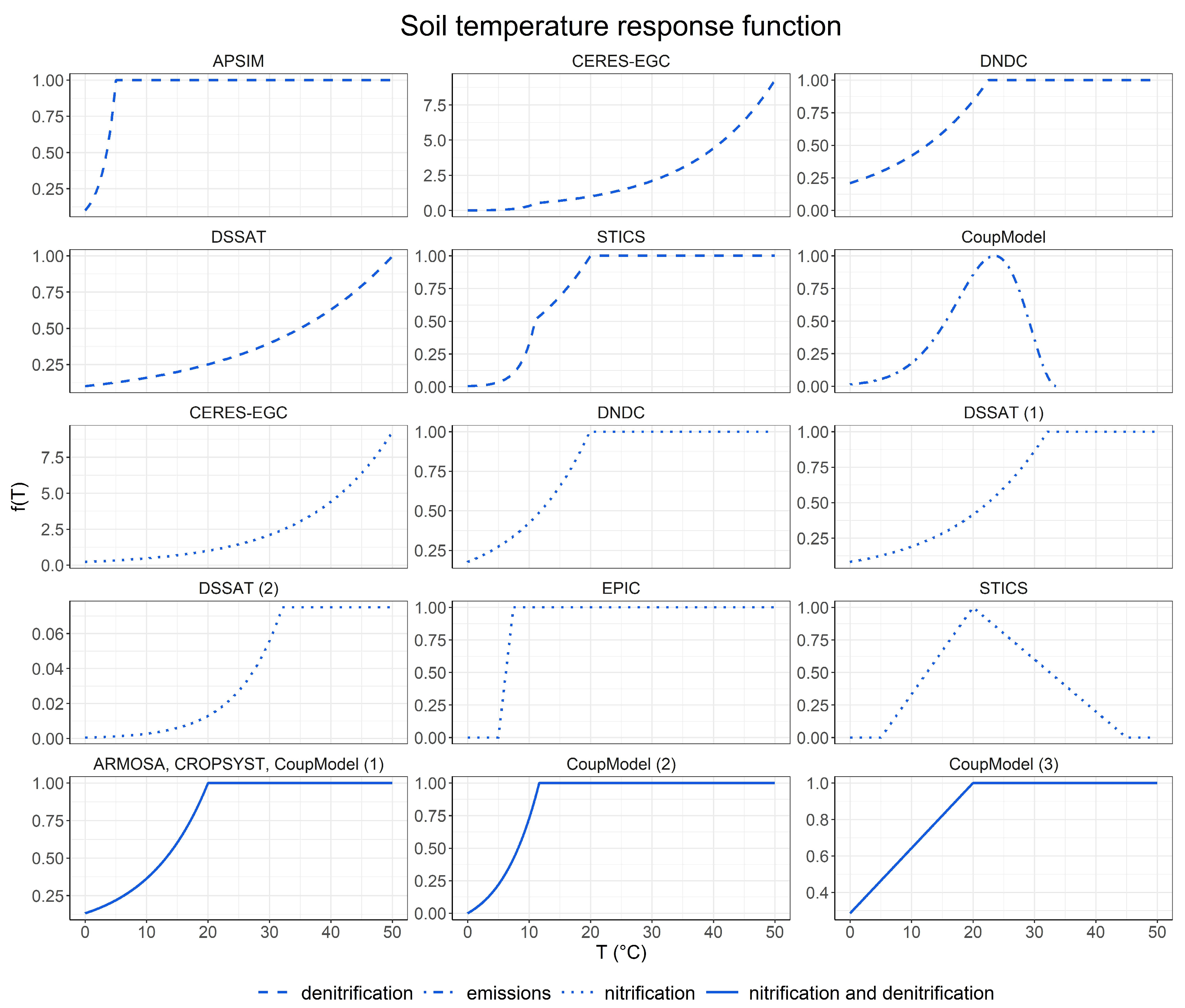
Soil Temperature Factor

In the APSIM model [67], the temperature factor limiting nitrification is the same as that used for the mineralization estimate [72]. It consists of an exponential function, whose minimum value (0) is obtained for a 0 °C soil temperature and whose maximum value (1) is obtained for a 30 °C soil temperature [84]. The temperature factor (Figure 1, Equation (40)) limiting denitrification is an exponential function of the soil temperature (T, °C) [67].
f d T = 0.1   ·   e ( 0.46   · T )  
In the ARMOSA model, the same soil temperature factor (f(T), unitless, Equation (41)) is employed both for nitrification and denitrification, and it is derived from the SOILN approach [75]. It consists of an exponential function, constrained between 0 and 1, having a Q10-value as a base (tQ10, unitless, between 1.5 and 4) that describes the response to a 10 °C soil temperature change. A base temperature (Topt, °C, 20) at which the temperature effect is equal to 1 is also employed. CROPSYST model [59,69,73] employs the same response function (Equation (41)) to limit only the nitrification rate.
f ( T ) = t Q 10 T T o p t 10
In the SPACSYS model [71], a Q10 equation having different Q10 for the various processes is employed, while in DAYCENT model 4.7 [11], the response function of nitrification to soil temperature, fn(T), is represented by a generalized Poisson density function.
In CERES-EGC [76], the response function of nitrification to soil temperature (T, °C) is an exponential function (Equation (42)) that is not limited to 1 and employs a Q10 factor parameter (tQ10, unitless, 2.1) describing the relative increase in the process activity for a 10 °C increase in soil temperature.
f n T = e T 20 · l n t Q 10 10
The exponential response function of denitrification to soil temperature (Equation (43)) is not limited to 1 and employs a threshold temperature parameter (Tdenit, °C, 11) and two Q10 factors: one for low temperature (tQ10,1, unitless, 89.0) and one for high temperature (tQ10,2, unitless, 2.1).
f d T = e T T d e n i t · l n t Q 10 , 1 9 l n t Q 10 , 2 10 i f   T < T d e n i t e T 20 · l n t Q 10 , 2 10 i f   T T d e n i t
In CoupModel [68], the response function of denitrification and of nitrification to soil temperature (T, °C, for the topsoil layer, it is equal to the air temperature) in a considered layer can be selected among three different options (Figure 1, Equation (44)). A function that becomes a Q10-type function above a certain temperature threshold (f(T)1), a Q10-type function for the whole range of temperatures (f(T)2), and a Ratkowsky function consisting in a quadratic function (f(T)3). The employed parameters are the following: response to a 10 °C soil temperature change on the microbial activity, nitrification and denitrification (tQ10, unitless, 2), base temperature for the microbial activity, nitrification and denitrification at which the response is 1 (Topt, °C, 20), threshold temperature for the microbial activity, nitrification and denitrification below which the response is stronger than above and ceases at 0 °C (TQ10thres, °C, 5), minimum temperature for nitrification and denitrification (Tmin, °C, −8), and temperature at which the response of nitrification and denitrification is equal to 1 (Tmax, °C, 20).
f T 1 = t Q 10 T T o p t 10 f T 2 = T T Q 10 t h r e s · f d T 1 f ( T ) 3 = 1 i f   T > T m a x T T m i n T m a x T m i n 2 i f   T m i n < T < T m a x   0 i f   T < T m i n
The response function (fe(T), unitless, Equation (45)) to soil temperature for N2O and NO emissions during nitrification employs three parameters: the maximum (gTmaxNxO, °C, 33.5) and optimum (gToptNxO, °C, 23.5) soil temperature for the formation of nitrous trace gases during nitrification, and the parameter determining the response function shape (gTshapeNxO, unitless, 1.5).
f e ( T ) = g T m a x N x O T g T m a x N x O g T o p t N x O f ( T e x p ) f ( T e x p ) = g T s h a p e N x O · T g T o p t N x O g T m a x N x O g T o p t N x O
In DNDC model version 9.5 [79], the soil temperature (T, °C) factor employed in the nitrification is an exponential function of soil temperature (Figure 1, Equation (46)).
f n T = 3.503 ( 60 T ) 25.78 · e 3.503 · ( T 34.22 ) 25.78
The soil temperature factor employed in the denitrification estimate (Figure 1, Equation (47)) is a Q10-type function with a base equal to 2 and an optimum temperature of 22.5 °C, with a soil temperature threshold parameter (Tmax,denit, °C, 60). The function is equal to zero when the soil temperature is higher than the threshold value.
f d T = 2 T 22.5 10             i f   T T m a x , d e n i t
In DSSAT model [70] V4.8.2.0 [77], two functions are used for the response of nitrification to soil temperature: the first one is constrained between 0 and 1 and describes soil temperature (T, K) effect on nitrification (fn1(T), unitless, Figure 1, Equation (48)), while the second one is a function (fn2(T), unitless, Figure 1, Equation (48)) of the temperature response function of the previous time step (fn1(T)t−1, unitless).
f n 1 T = e 6572 T + 21.4 f n 2 T = m i n 0.075 · f n 1 T t 1 2 , 1
The response function of denitrification to soil temperature (T, K) is only present in the CERES denitrification subroutine, and it is limited between 0 and 1 (fd(T), unitless, Figure 1, Equation (49)).
f d T = 0.1 · e 0.046 · T
In EPIC model [62] v. 1102 [78], the response function of nitrification to soil temperature (T, °C) is a linear function (Equation (50)).
f n T = 0.41 · ( T 5 )
In the STICS model [60], the response function of nitrification to soil temperature (T, °C) is limited between 0 and 1 (Figure 1, Equation (51)), and it is defined by the following parameters: minimum cardinal temperature for nitrification (Tmin,nit, °C), optimum cardinal temperature for nitrification (Topt,nit, °C), and maximum cardinal temperature for nitrification (Tmax,nit, °C).
f n T = T T m i n , n i t T o p t , n i t T m i n , n i t   i f   T T o p t , n i t T T m a x , n i t T o p t , n i t T m a x , n i t   i f   T T o p t , n i t
The response function of denitrification to soil temperature (T, °C) is limited between 0 and 1 (Figure 1, Equation (52)), and it is defined by two cardinal temperatures for denitrification (T1,denit, °C, 11; T2,denit, °C, 20).
f d T = e T T 1 , d e n i t · 0.449 0.668 i f     T T 1 , d e n i t   e T T 2 , d e n i t · 0.0742 i f     T > T 1 , d e n i t

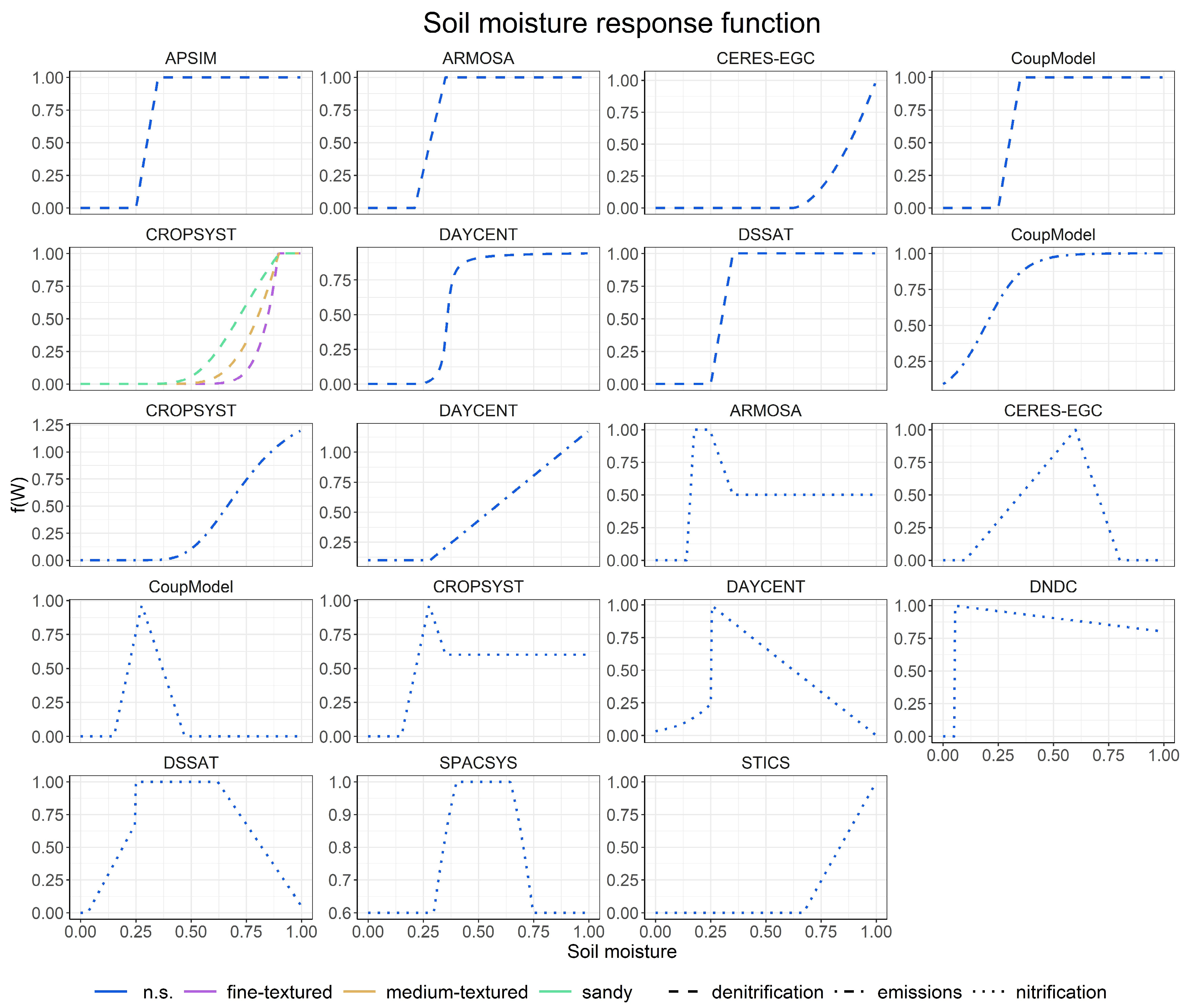
Soil Moisture Factor

In the APSIM model [67], the soil moisture factor limiting nitrification is a trapezoidal function whose value is 0 at the lower limit soil water content and at the saturation soil water content (SWCsat), and it is equal to 1 at the drained upper limit. All the considered soil water contents are volumetric ones [84]. The soil moisture factor limiting denitrification (Figure 2, Equation (53)) is defined by the following parameters: water content at which denitrification ceases (SWClim, in the default configuration, is equal to the value of WFPS at DUL) and empirical coefficient (x, in the default configuration equal to 1) [67].
f d W = S W C S W C l i m S W C s a t S W C l i m x
In ARMOSA, the soil moisture effect on nitrification is described through a response function (fn(W), unitless, Figure 2, Equation (54)) limited between 0 and 1, which employs four soil water content thresholds (SWCmin, SWCoptmin, SWCoptmax, and SWCmax, m3 m−3, Appendix A.2, Appendix A) that are estimated as fractions of the saturation water content (SWCsat, m3 m−3). The function is defined by the following parameters: microbial activity below SWCmin (fmin, unitless, 0), microbial activity above SWCmax (fmax, unitless, 0.5), microbial activity curvature coefficients (a and b, unitless, 1). When SWCSWCmin, the response function is equal to fmin; when SWC > SWCmax, the response function is equal to fmax, while the function is equal to 1 when SWC is comprised between SWCoptmin and SWCoptmax.
f n ( W ) = f m i n + 1 f m i n · S W C S W C m i n S W C o p t m i n S W C m i n a 1 f m a x + 1 f m a x · S W C m a x S W C S W C m a x S W C o p t m a x b 2 1   S W C m i n < S W C S W C o p t m i n 2   S W C o p t m a x < S W C S W C m a x
The soil moisture effect on denitrification is described through a response function, constrained between 0 and 1 (fd(W), unitless, Figure 2, Equation (55)), that is derived from the APSIM approach (Equation (53)). This response function uses three parameters: the saturation threshold (thrsat, unitless, 0.6), an empirical coefficient (x, unitless, 1, between 0.9 and 5), and a lower threshold for soil water content (thrdenit, unitless, 0.05) under which no denitrification occurs (response function equal to 0).
f d ( W ) = S W C t h r s a t · S W C s a t S W C s a t t h r s a t · S W C s a t x    
In CERES-EGC [76], the nitrification response function to soil water content (Equation (56)) increases linearly from a minimum WFPS value (WFPSmin,nit, %, 0.1) to an optimum value (WFPSopt,nit, %, 0.6). The function then decreases linearly to a maximum value (WFPSmax,nit, %, 0.8). It is equal to zero otherwise.
f n W = W F P S W F P S m i n , n i t W F P S o p t , n i t W F P S m i n , n i t   i f   W F P S m i n , n i t < W F P S W F P S o p t , n i t   W F P S m a x , n i t W F P S W F P S m a x , n i t W F P S o p t , n i t i f   W F P S o p t , n i t W F P S < W F P S m a x , n i t  
The denitrification response function to soil water content (Equation (57)) is equal to zero when the soil WFPS is lower than a threshold value (WFPSdenit, %, 0.62); otherwise, it consists of a function having a parameter as exponent (x, unitless, 1.74).
f d W = W F P S W F P S d e n i t 1 W F P S d e n i t x i f   W F P S W F P S d e n i t
In CoupModel [68], the soil moisture response function for denitrification (Figure 2, Equation (58)) is estimated differently on the base of the simulated soil water content (SWC, m3 m−3) and of the soil water content at saturation (SWCsat, m3 m−3). The response function is defined by the following parameters: a coefficient in the function for soil moisture effect on denitrification (pθDp, unitless, 10) and a water content range from saturation in the function for soil moisture on denitrification (pθDRange, %, 10). The function is equal to 1 when SWC is equal to SWCsat, while it is equal to zero when SWCSWCsat > pθDp.
f d W = S W C S W C s a t p θ D R a n g e p θ D R a n g e p θ D p                         i f   S W C S W C s a t < p θ D p
The soil moisture response function for nitrification (Figure 2, Equation (59)) is estimated differently on the base of the simulated soil water content at saturation and at wilting point (SWCwilt, m3 m−3) and is defined by the following parameters: saturation activity in soil moisture response function (pθsatact, unitless, 0.6, 0 is equal to no activity, 1 is equal to optimum activity at saturation), water content interval lower limit in the soil moisture response for nitrification and denitrification (pθLow, %, 13, range 8–15), the coefficient for the soil moisture function (pθp, unitless, 1 corresponds to a linear response, 0–1 corresponds to a convex response, >1 corresponds to a concave response), water content interval upper limit in the soil moisture response function for nitrification and denitrification (pθUpp, %, 8, range 1–10). The function is equal to pθsatact when SWC is equal to SWCsat, while it is equal to zero when SWC < SWCwilt.
f n W = m i n S W C s a t S W C p θ U p p p θ p · 1 p θ s a t a c t + p θ s a t a c t S W C S W C w i l t p θ L o w p θ p  
In the CROPSYST model [59,69,73], the response function of nitrification (Figure 2, Equation (60)) to the volumetric soil water content (SWC, m3 m−3) is modeled with the SOILN approach [74,75]. The response function is equal to zero below the wilting point (SWCwilt, %); it increases to one in the interval delimited by a parameter (pθLow, %, 13), and near the saturation water content (SWCsat, %), it decreases to a saturation activity (pθsatact, unitless, 0.6, range 0–1) in an interval confined by a parameter (pθUpp, %, 8). The shape of the response curve between pθLow and pθUpp is given by a parameter (pθp, unitless), the linear response is obtained with a value of 1; between 0 and 1, the response function is convex, and for values higher than 1, the response is concave. pθLow is the water content interval defining increasing activity from 0 (no activity) at SWCwilt to 1 (optimum activity) at pθLow + SWCwilt; its normal range is 8–15, depending on soil type. pθUpp is the water content interval defining decreasing activity from 1 (optimum activity) at SWCsatpθUpp to the activity given by parameter pθsatact at SWCsat; its normal range is 1–10, depending on soil type.
f n W = p θ s a t a c t + 1 p θ s a t a c t · S W C s a t S W C p θ U p p p θ p   1 S W C S W C w i l t p θ L o w p θ p                     2 1   i f S W C s a t p θ U p p < S W C < S W C s a t 2   i f   S W C w i l t < S W C < S W C w i l t + p θ U p p
The response function (fd(W), unitless, Equation (61)) describing WFPS (unitless) effect on denitrification is limited, between 0 and 1 [80], its parameters values vary with soil texture (sandy, medium and fine): a (1.56, 4.82, and 60.0), b (12.0, 14.0, and 18.0), c (16.0, 16.0, and 22.0), and d (2.01, 1.39, and 1.06).
f d W = a b c b ( d · W F P S )
In DAYCENT model 4.7 [11], the response function of nitrification and denitrification, fn(W) and fd(W), consider the second and the third soil layer moisture status only (Figure 2). The response function for nitrification (Equation (62)) employs available soil water content (SWCavail, m3 m−3) and the weighted average of the WFPS of the considered layers, respectively, for soils drier or wetter than field capacity (SWCfc, m3 m−3).
f n W = 1 1 + 30 · e 9 · S W C a v a i l i f   S W C S W C f c 1 1 S W C f c · W F P S a v g 1 e l s e
The WFPS curve (Equation (63)) of the denitrification submodel [81] was modified [11] to stop the denitrification process for WFPS < 55%, and it is defined by a parameter corresponding to the WFPS level at which the denitrification reaches half of its maximum velocity (a, unitless). The WFPS [11,85] for the two response functions is calculated as a function of gravimetric soil water content (θg, g water g soil−1) and bulk density (BD, g cm−3).
f d W = 0.45 + a t a n 0.6 · π · 0.1 · W F P S a π W F P S = θ g · B D 1 B D 2.65
In DNDC model version 9.5 [79], a soil moisture factor (Figure 2, Equation (64)) is employed in the nitrification estimate, for which the soil water content is expressed as water-filled porosity (WFPS).
f n W = 0.8 + 0.21 · 1 W F P S i f   W F P S > 0.05   0 i f   W F P S 0.05
In DSSAT model [70] V4.8.2.0 [77], the response function (fn(W), unitless, Figure 2, Equation (65)) of nitrification to soil water content (SWC, m3 m−3) is based on water-filled porosity (WFPS, unitless), and it is limited between 0 and 1. The function uses as soil water content thresholds the drained upper limit (DUL, m3 m−3) and the saturation water content (SWCsat, m3 m−3). The WFPS is obtained as the ratio between SWC and SWCsat.
f n W = 2.5 · W F P S + 2.55 i f   S W C > D U L 1 i f   S W C < D U L   a n d   W F P S > 0.4 3.15 · W F P S 0.1 e l s e
In the DAYCENT denitrification subroutine, the response function of denitrification (fd(W), unitless, Equation (66)) to soil moisture is constrained between 0 and 1 and considers the soil gas diffusivity at field capacity (gdiff, unitless), the WFPS and an auxiliary variable (CO2correct, Equation (91)).
f d W = 0.45 + a t a n 0.6 · π · 10 · W F P S 9.0 M · C O 2 c o r r e c t π M = m i n 0.113 ,   g d i f f · ( 1.25 ) + 0.145  
In the CERES denitrification subroutine, the response function of denitrification (fd(W), unitless, Equation (67)) to soil moisture is constrained between 0 and 1 and is calculated when soil moisture (SWC, m3 m−3) is higher than the drained upper limit (DUL, m3 m−3).
f d W = 1 S W C s a t S W C S W C s a t D U L
In EPIC model [62] v. 1102 [78], the Armen Kemanian denitrification method employs a water factor (fd(W), Equation (68)) that considers the soil layer porosity (PO, m3 m−3), its soil water storage (SWT, m3 m−3, fraction of field capacity), its thickness (zlayer, m), and its clay amount (CLAY, %).
f d W = 1 1 + 1 A I R V 0.9 + 0.01 · C L A Y 60 i f   1 A I R V 0.9 + 0.01 · C L A Y > 0.8 0 e l s e     A I R V = P O S W T z l a y e r
In the SPACSYS model [71], the water-filled pore space (WFPS) response function is applied only to nitrification (Figure 2, Equation (69)), and it is expressed with a quadratic function, with the WFPS estimate approach derived from [86,87]. Its value depends on volumetric soil water content (SWC, m3 m−3), soil bulk density (BD, g cm−3), and soil particle density (PD, g cm−3) parameters.
f n W = m i n 1 ; 11.25 · W F P S 2 + 11.75 · W F P S 1.9   i f   0.3   W F P S 0.75 0.6   i f   0.3 < W F P S   o r   W F P S > 0.75 W F P S = S W C 1 B D P D
In the STICS model [60], the response function (Equation (70)) of nitrification to soil water content (SWC, mm water cm−1 soil) is limited between 1 and 0, and it employs an optimal water content parameters (SWCopt,nit, unitless, 1) that is different from the one used for mineralization, and a minimal soil water content for nitrification process (SWCmin,nit, unitless, 0.67). All the soil water content parameters are expressed as a proportion of field capacity water content (SWCfc, mm water cm−1 soil).
f n W = S W C S W C m i n , n i t · S W C f c S W C o p t , n i t S W C m i n , n i t · S W C f c
The response function of denitrification to soil moisture is defined using the auxiliary variable saturation soil status (WFPS, unitless), and it is related to the mineralization process through the reference temperature for soil mineralization parameter (Tminer, °C, 15). The function (Figure 2, Equation (71)) is limited between 0 and 1. It considers the amount of water remaining in the soil macroporosity (SWCsat, mm) and the bulk density (g cm−3).
f d W = W F P S 0.62 T T m i n e r 100 1 0.62 T T m i n e r 100 1.74   W F P S = S W C + S W C s a t 10 · 1 B D 2.66
In the CROPSYST model [59,69,73], the response function (fe(W), unitless, Equation (72)) describing the WFPS (unitless) effect on N2/N2O ratio for denitrification gas fluxes is not constrained between 0 and 1, and it is derived from [80].
f e W = 1.4 13 17 13 2.2 · W F P S
In DAYCENT model 4.7 [11], a WFPS effect on the N2/N2O ratio (fe(W), Equation (73)) is also applied.
f e W = m a x 0.1 ,   0.015 · W F P S · 100 0.32
In CoupModel [68], the soil moisture response function limiting the production of NO and N2O during nitrification (fe(W), unitless, Equation (74)) is defined by two parameters: the relative saturation level in the response function for soil moisture when NO or N2O is formed during nitrification (gθsatcrit, unitless, Table A8, Appendix A.3, Appendix A) and the parameter describing the shape of the moisture response function for NO or N2O emissions (gθsatform, unitless, Table A8, Appendix A.3, Appendix A).
f e W = 1 1 1 + e S W C / S W C s a t g θ s a t c r i t g θ s a t f o r m

Soil Acidity Factor

In the APSIM model [67], the soil acidity factor limiting nitrification is a trapezoidal function [84] whose value is equal to 0 when pH < pHmin (unitless, 4.5) or pH > pHmax (9, unitless) and whose value is equal to 1 for pHoptminpHpHoptmax (unitless, 6 and 8, respectively). The response function of nitrification to soil acidity in ARMOSA, CROPSYST [59,69,73], and STICS [60] models employs the SOILN approach [74,75]: it is a linear function (Figure 3, Equation (75)) defined by two parameters. The function is equal to 0 for pH < pHmin (unitless, 3), while it is equal to 1 for pH > pHmax (unitless, 5.5).
f n p H = p H p H m i n p H m a x p H m i n
In CoupModel [68], the response function of denitrification (Figure 3, Equation (76)) to soil acidity is defined by two parameters: the pH half rate (dpHrate, unitless, 4.25) and a shape coefficient (dpHshape, unitless, 0.5).
f d p H = 1 1 1 + e p H d p H r a t e d p H s h a p e
In CoupModel [68], the response function of NO and N2O production during nitrification to soil acidity (Equation (77)) employs a parameter (pHmin, unitless, 4.7) describing the pH value below, in which the function is equal to 1.
f e p H = p H m i n p H
In DAYCENT model 4.7 [11,85], the response function of nitrification to soil acidity (Equation (78)) is calculated as an inverse function of the tangent function (atan is a standard C arctangent function from the library math.h).
f n p H = atan ( p H ,   a )
In DNDC model version 9.5 [79], a pH factor for denitrification is employed (fd(pH)NxOy, Figure 3, Equation (79)).
f d p H N x O y = 1 1 e ( p H 4.25 ) / 0.5   i f   N x O y = N O 3   1 1 e p H 5.25 / 1   i f   N x O y = N O 2   o r   N O 1 1 e p H 6.25 / 1.5   i f   N x O y = N 2 O
In DSSAT model [70] V4.8.2.0 [77], the response function of nitrification to soil acidity (fn(pH), unitless) is limited between 0 and 1. It is equal to 0 and 1 when pH < pHmin and when pH > pHopt, respectively, and linear in between (Figure 3, Equation (80)).
f n p H = m i n ( 1 ,   0.33 · p H 1.36 )
In EPIC model [62] v. 1102 [78], a trapezoidal response function (Figure 3, Equation (81)) of nitrification to soil acidity (pH, unitless) is employed: it is constrained between 0 and 1 and defined by two parameters: pH optimum minimum threshold (pHoptmin, unitless, 7) and pH optimum maximum threshold (pHoptmax, unitless, 7.4).
f n p H = 0.307 · p H 1.269 i f   p H < p H o p t m i n 1 i f   p H o p t m i n p H p H o p t m a x 5.367 0.599 · p H i f   p H > p H o p t m a x
In the SPACSYS model [71], the response functions of nitrification and denitrification to soil acidity are unitless and limited between 0 and 1 (each step of the denitrification process presents its own function, Figure 3, Equation (82)).
f n p H = e p H 6.6 2 2 f d , N O 3 p H = 1 1 1 + e p H 4.25 0.5 f d , N O p H = 1 1 + e p H 4.5 2.5 5.5 f d , N O 2 p H = e p H 6.2 2 2 f d , N 2 O p H = e p H 8.2 2 2

Substrate Concentration Effect

In CERES-EGC [76], the response function of nitrification (Equation (83)) to soil ammonium content (mg N kg soil−1) employs a half-saturation constant parameter (Km,nit, mg N kg soil−1, 10) that is modified on the base of the soil water content value.
f n N H 4 = N H 4 K m , n i t · S W C + N H 4
In the response function of denitrification (Equation (84)) to soil nitrate content (mg N kg soil−1), using a dedicated half-saturation constant (Km,denit, mg N kg soil−1, 22), the soil water content is not considered.
f d N O 3 = N O 3 K m , d e n i t + N O 3
In CoupModel [68], the response function of denitrification (Equation (85)) to nitrate concentration ([NO3], mg N L−1) employs a parameter describing the half-saturation constant (Km, mg N L−1, 10, range 5–15), i.e., the nitrate concentration at which the activity is half of the activity at optimum nitrate concentration.
f d N O 3 = N O 3 S W C · z l a y e r N O 3 S W C · z l a y e r + K m
The response function of nitrification rate (Equation (86)) to nitrate and ammonium ([NH4], mg N L−1) concentrations in the simplified approach, i.e., when microbes are not considered, employs two parameters: the nitrate–ammonium ratio (rNO3/NH4, unitless, 8, range 1–15) and the specific nitrification rate (knit, d−1, 0.2).
f n N H 4 , N O 3 = m a x 0 ,   N H 4 N O 3 r N O 3 / N H 4 · k n i t
The response function of nitrification rate (Equation (87)) to ammonium concentration in the microbial biomass explicit approach employs the nitrification half rate parameters (Km, mg N L−1, 6.18).
f n N H 4 = N H 4 S W C · z l a y e r N H 4 S W C · z l a y e r + K m
In CROPSYST [59,69,73], the response function (fd(NO3), g N ha−1 d−1, Equation (88)) describing the maximum denitrification for a certain NO3 (µg N g−1) soil level is derived from [80].
f d N O 3 = 11.00 + 40.00 · a t a n π · 0.002 · ( N O 3 180 ) π
The response function (fd(CO2), g N ha−1 d−1, Equation (89)) describing the maximum denitrification for a certain soil respiration (CO2,resp, kg C N ha−1 d−1) level is derived from [80].
f d C O 2 = 24 1 + 200 e 0.35 · C O 2 , r e s p 100
In DAYCENT model 4.7 [11], the two substrate concentration effect functions (fd(NO3), fd(CO2), µg N g soil−1 d−1, Equation (90)) are not limited between 0 and 1 (they cannot be negative), but they correspond to the potential total N flux not limited by CO2 and H2O for fd(NO3) by NO3 and H2O for fd(CO2) [81].
f d N O 3 = a t a n N O 3 , a f d C O 2 = 0.1 · C O 2 1.3 0.1
In DSSAT model [70] V4.8.2.0 [77], the DAYCENT denitrification subroutine employs a denitrification response function to NO3 (fd(NO3), kg N ha−1 d−1, Equation (91)) that has a lower bound equal to zero.
f d N O 3 = 1.556 + 76.91 π · a t a n π · 0.00222 · ( N O 3 9.23 )
In the DAYCENT denitrification subroutine, the denitrification response function to CO2 (fd(CO2), unitless, Equation (92)) is derived from [81] and has a lower bound equal to zero. It considers a minimum amount of nitrate (NO3,min, kg N ha−1 d−1, 0.1) and an auxiliary variable (CO2correct, Equation (91)), derived from the CO2 produced daily (CO2,resp) in the first two soil layers (first soil layer, L = 0, and second soil layer, L = 1, the first soil layer also includes the mulch layer).
f d C O 2 = 0.1 ·     C O 2 c o r r e c t 1.3 N O 3 , m i n C O 2 c o r r e c t = C O 2 i f   W F P S t h r W F P S C O 2 · 1 + a · ( W F P S t h r W F P S ) e l s e C O 2   ( L ) = C O 2 ,   r e s p 0 + C O 2 ,   r e s p 1 i f   L = 1 C O 2 ,   r e s p L e l s e t h r W F P S = 0.8   i f   g d i f f 0.15 g d i f f · 250 + 43 100   e l s e a = 0.004 i f   g d i f f 0.15 0.1 · g d i f f + 0.019 e l s e
In the CERES denitrification subroutine, the water-extractable soil carbon amount (CW, Equation (93)) depends on the availability of C from the humic fraction (CSSOM) and of the fresh C from the carbohydrate pool (CLIT).
C W = 24.5 + 0.0031 · C S S O M + 0.2 · C L I T
In EPIC model [62] v. 1102 [78], the Armen Kemanian denitrification method uses a nitrate factor (fd(NO3), Equation (94)).
f d N O 3 = m a x 1 e 5 , 1000 · N O 3 W T m a x 1 e 5 , 1000 · N O 3 W T + 60
In the Armen Kemanian denitrification method, the respiration factor (fd(CO2), Equation (95)) considers the CO2 respiration (CO2,resp, kg C N ha−1 d−1) of the layer and the soil weight (WT).
f d C O 2 = m i n 1 ,   1000 · C O 2 , r e s p W T 50
In the SPACSYS model [71], the substrate concentration effects, fd(DOC), fd(NO3), and fn(NH4) are described by a Michaelis–Menten-like equation (Equation (96)), and they depend on substrate concentration ([S], g C m−3 or g N m−3) and on the Michaelis constant for the substrate (Km, g C m−3 or g N m−3). The constant default values are 9.45, 16.65, and 18.53, respectively, for DOC, NO3, and NH4+.
f [ S ] = [ S ] [ S ] + K m
In the STICS model [60], nitrate (NO3, kg N ha−1 cm−1) concentration effect on denitrification (Equation (97)) also depends on soil bulk density (BD, g cm−3).
f d ( N O 3 ) = N O 3 N O 3 + 2.2 · B D
In the DAYCENT denitrification subroutine DSSAT model [70] V4.8.2.0 [77], a nitrate effect on the N2/N2O ratio (fe(NO3), Equation (98)) is also applied.
f e N O 3 = m a x 0.16 · K 1 , K 1 · e 0.8 · N O 3 C O 2 c o r r e c t   i f C O 2 > 0.001   0.16 · K 1 e l s e K 1 = m a x 1.5 ,   38.4 350 · g d i f f
In the CROPSYST model [59,69,73], the response function (fe(NO3), Equation (99), unitless, not constrained between 0 and 1) describing NO3 (µg N g−1) effect on N2/N2O ratio for denitrification gas fluxes is derived from [80].
f e N O 3 = 1 0.5 + 1 · a t a n π · 0.01 · N O 3 190 π · 25
The response function (fe (CO2), Equation (100), unitless, not constrained between 0 and 1) describing soil respiration (CO2,resp, kg C N ha−1 d−1) effect on N2/N2O ratio for denitrification gas fluxes is derived from [80].
f e C O 2 = 13 + 30.78 · a t a n π · 0.07 · ( C O 2 , r e s p 13 ) π

3.1.5. Model Evaluation

This section evaluates 8 (i.e., APSIM, CERES-EGC, CoupModel, DAYCENT, DNDC, EPIC, SPACSYS, and STICS) of the reviewed models, for which the model assessment of N2O simulation performance was available in published articles. Due to limited data availability of the following models’ application and evaluation, CROPSYST, DSSAT, and ARMOSA, were not included in this section. In total, we analyzed 16 papers (Table 2) related to the application of these models, with 10 aimed at validation, 3 at calibration, and 3 reporting the results of both evaluation processes. The 83% of these papers were published between 2015 and 2023. In these studies, measured N2O emissions were derived both from field and laboratory experiments conducted by the authors of the articles and from experiments carried out by other researchers. The experiment sites were categorized according to the Köppen climate classification, considering their geographical positions, to obtain an overview of the climatic conditions in which the experiments and the simulations were carried out. The most common climatic group that emerged was Cfb, corresponding to a temperature of the warmest month greater than or equal to 10 °C, and temperature of the coldest month less than 18 °C but greater than 3 °C, and precipitation evenly distributed throughout the year [88].
In more than half of the studies, measurements of N2O emissions in the field were conducted intermittently (i.e., not-continuous measurements). Most of the studies that employed intermittent measurement approaches dealt with a large number of experimental treatments. In contrast, in studies where measurements were taken continuously, the maximum number of tested treatments was limited to 4. Simulated and measured N2O emissions were reported by the individual studies both as cumulative and daily values. More in detail, 7 of the reviewed model evaluations used cumulated N2O emissions, 9 used both cumulated and daily N2O emissions, and 4 employed only daily N2O emissions.
A comprehensive overview of the statistical indices extracted from the studies is reported in Table A9 (Appendix A.3, Appendix A), and it is organized according to the treatment(s) for which they were calculated. The most frequently reported index in the reviewed studies, determination coefficient (R2), allowed us to compare model performances concerning both cumulated and daily emissions. Other performance indices (r, RMSE, RRMSE, EF) were seldom used. Furthermore, the different time periods employed to obtain cumulated N2O emissions values and the associated RMSE values prevented the possibility of this accuracy index comparisons, while relative errors (RRMSE) were rarely reported.
In general, the reported determination coefficient values are higher when estimated with cumulated N2O emissions values than the ones obtained from daily values (Figure 4). When considering the combination of measure methodology (continuous and not-continuous measures) and model output (daily and cumulated emissions), differences in models’ performance are more relevant for validation studies than for calibration ones (Table A9). In the reviewed studies, the average R2 obtained after calibration with continuous measures corresponds to 0.48 (with R2 values reported for daily emissions ranging from 0.31 to 0.56 and from 0.30 to 0.67 for cumulated emissions), while it is equal to 0.65 for calibration studies that employed not-continuous measures (0.1–0.92 and 0.41–0.96, respectively, for daily and cumulated emissions). The average R2 value, deriving from the published validation coefficient of determinations, were equal to 0.55 and 0.29, respectively, for continuous (0.05–0.74 and 0.4–0.95, respectively, for daily and cumulated emissions) and not continuous (0.02–0.5 and 0.02–0.89, respectively, for daily and cumulated emissions) measures. Frequently, models that were calibrated with continuous measures obtained higher R2 when subjected to validation using the same type of measured data (particularly when the fitting index is calculated on cumulated emissions). The choice between using cumulated or daily values appears to be primarily linked to measured data frequency, which is associated with the specific research objectives and resource availability. It should be noted that the use of cumulated emissions values for model evaluation tends to reduce the disagreement between measured and simulated data, which can represent both an advantage and a disadvantage. Indeed, the use of cumulated values allows for obtaining higher determination coefficients in the calibration phase, but it does not always ensure the same results at validation (particularly when carried on independent datasets). Conversely, daily emissions values provide a more detailed view but may reveal greater discrepancies between observations and simulations (Table A9).
When considering only mineral N fertilization treatments, as expected, R2 values reported in calibration studies that employed not-continuous measures (average R2 0.66) are higher than the ones obtained after calibration with continuous measures (average R2 0.48). In validation studies simulating these treatments, average R2 values were, however, higher in studies that employed continuous measures (0.46) than in the ones that used not-continuous measures (0.27). Probably, this difference is due to the fact that studies that employed continuous emissions measures for validation purposes also employed model parameter sets calibrated on continuous emissions. Determination coefficients deriving from the reviewed zero N control treatments were generally low (average R2 equal to 0.065 and 0.31, respectively, for continuous and not-continuous measures) since they were estimated for validation datasets of daily emissions.

4. Discussion

From the appraisal of the main approaches for N2O emissions modeling, and in agreement with [54], it emerged that soil and weather conditions variability representation is the main driver employed for describing the interactions network that connects soil chemical–physical properties and weather conditions to soil N cycling and the consequent gaseous emissions. In the reviewed process-based models, the level of detail of weather variability representation is obtained by the adoption of a daily time step and of specific parameter values for each simulated process, thus differentiating these approaches from the statistical ones (e.g., IPPC guidelines and statistical models). Soil physical properties are adequately described by the employment of soil hydrological parameters, which allows the simulation of soil water content and temperature variations as influenced by weather trends, soil cover type (bare soil, vegetal soil cover derived from crop growth and development modules) and soil tillage operations. Differences in WFPS simulation or in soil hydrological parameters calculation arise from each model’s specific characteristics. The reviewed algorithms generally estimate nitrification and denitrification rates as potential rates limited by soil temperature and moisture response functions, both for the implicit and explicit microbial pool approaches. The main differences that lead to simulated output behaviors, specifically after calibration, are given by the formalization of response functions. Nitrification, in the majority of the approaches, is also limited by soil acidity, while denitrification in the implicit microbial pools approaches is influenced by soil respiration. Indeed, soil organic carbon pool simulation contributes to improving the quality of N2O emissions representation in process-based models since it allows a more detailed description of the soil mineral nitrogen fluxes. When microbial biomass is explicitly simulated, nitrification and denitrification rates are directly proportional to the microbial biomass itself.
With respect to other types of modeling approaches, process-based models also allow daily representations of management operations (tillage, organic and mineral fertilization, irrigation, residue retention, or removal) and their influence on soil C and N cycles in a specific soil layer. The majority of the reviewed approaches employ dynamic assessment of the fraction of nitrified or denitrified N that is lost as N2O, and in some cases, further emissions response functions to soil conditions are considered. The major limitation of the IPCC methodology, also shared by statistical models, is not being representative of the reality of crop and soil dynamics since environmental factors influence, and their spatial–temporal heterogeneity is not taken into account. Emission factors, produced by the application of IPCC guidelines, rely on simpler relations that assume a linear proportionality between the N mineral pool and nitrous oxide emission. While this approach is straightforward and of universal applicability, it might lead to sensible underestimation or overestimation of the total emission in case of deficiency or abundance in the N mineral pool, respectively.
Process-based approaches’ effectiveness largely depends on the quality and precision of the input data used for calibration and validation. As mentioned before [24,25,26,27,28], quantifying N2O emissions represents a challenge, primarily due to the spatio-temporal variability of fluxes. Therefore, the chosen methodology for measuring gas fluxes plays a crucial role. Measured data uncertainty, arising, for example, from linear interpolation of manual measurements, considerably impacts the model’s performance. On the other hand, the use of automated chambers in manipulative experiments demands intensive labor, advanced sensor technology, and proficient users, while long-term unattended observations of emission fluxes and environmental driver variables by networks of permanent micrometeorological observation sites are an easy way of disposing of datasets collected in contrasting environments for calibration, validation, and comparison.
To address this uncertainty, it is necessary to increase the quantity and accuracy of measurements, even though this requires significant efforts in data collection and processing [13,50,51] and in terms of resource availability.
However, as mentioned earlier, the use of automatic systems for measures acquisition requires complex technology adoption by expert users, often presenting challenges in terms of availability and resources. When such data are available, the models can effectively represent the phenomenon accurately [43]. The current availability of long-term continuous time series of semi-hourly GHG flux data—such as ICOS Carbon Portal (https://www.icos-cp.eu/, accessed on 16 November 2023) or FLUXNET2015 dataset (https://fluxnet.org/data/fluxnet2015-dataset/, accessed on 16 November 2023)—coupled with high-quality biophysical variables as well as ancillary data and metadata represents a useful tool for carrying on multiple model comparison exercises [100]. In this regard, subsets of data might be assembled from selected permanent ecological sites of worldwide networks and be the object of relative simulation confrontation of an ensemble of models. Another consideration arises from the variable diffusivity of N2O within the soil at different depths, making it challenging to select the appropriate simulation setup and, as a consequence, to calibrate according to measured values that are taken in the soil–atmosphere interface (usually a few centimeters depth from topsoil). This is a critical issue as the majority of selected papers do not provide information about the thickness of the topsoil layer to which the simulated emissions are referred.
One of the most used indicators of the agreement between simulated and observed data is the coefficient of determination, R2. However, it is important to note that an optimal R2 value (close to 1) does not necessarily guarantee the model’s ability to reproduce the processes accurately and efficiently. In the reviewed model evaluations, high R2 was frequently associated with discrete RMSE values, even if the latter are reported in a few studies. In general, it is good practice to use a combination of different criteria to address model performance evaluation, adopting a broader set of indices that evaluate several aspects of model performance [101]. To truly appreciate the efforts put into measuring and modeling N2O emissions, a set of model performance indices should be estimated for emissions and other N pools to allow a comprehensive evaluation of the modeling approaches.

5. Conclusions

In the present paper, we have undertaken a comprehensive examination of the main approaches for modeling N2O. The modeling approaches review was based on their operational principles, although consideration was also given to the model evaluation as presented in published articles. One of the main limitations of the N2O process-based modeling, underlined by this review, is connected to the inherent difficulties in the direct measure of emissions, which increases model evaluation process uncertainty. In particular, long-period field trials concerning representative cropping systems are required to support models’ calibration and improvement. Methodological limitations are also linked to the dynamic simulations of the other cropping system components (crop N uptake, soil organic matter pool evolution, and mineralization in particular) and their accuracy, efficiency, and robustness. This review schematically reports approaches and equations with the aim of easing the comparison of the mechanisms underlying the N2O emissions simulation. Given the increasing interest in N2O emissions and their environmental drivers in the agroecosystems, the application of process-based modeling to evaluate cropping system management practices constitutes a powerful tool, even with the abovementioned methodological limitations. Furthermore, process-based models allow the estimate of conditions-specific emission factors for given climate, soil, and cropping system (including annual or perennial crops) combinations that stakeholders (researchers, administrations, and farmers) can evaluate complementarily to IPCC emissions factors, thus deepening N2O emissions dynamics assessment. Given the uncertainty associated with N2O simulated emissions, an advisable approach is represented by multi-model ensemble applications to assess possible emissions ranges.

Supplementary Materials

The following supporting information can be downloaded at: https://www.mdpi.com/article/10.3390/horticulturae10010098/s1. Supplementary Materials: overview of the other N2O modeling approaches. Refs. [41,45,102,103,104,105,106,107,108,109,110,111,112,113,114,115,116,117] are cited in Supplementary Material.

Author Contributions

Conceptualization, M.G., M.A., G.R. and A.P.; methodology, M.G., M.A., G.R. and A.P.; investigation, M.G. and M.A.; writing—original draft preparation, M.G. and M.A.; writing—review and editing, G.R., A.M., L.V. and A.P.; supervision, G.R. and A.P. All authors have read and agreed to the published version of the manuscript.

Funding

This study was carried out within the Agritech National Research Center and received funding from the European Union Next-Generation EUGeneration EU (PIANO NAZIONALE DI RIPRESA E RESILIENZA (PNRR)—MISSIONE 4 COMPONENTE 2, INVESTIMENTO 1.4—D.D. 1032 17 June 2022, CN00000022). This manuscript reflects only the authors’ views and opinions, and neither the European Union nor the European Commission can be considered responsible for them.

Data Availability Statement

No new data were created or analyzed in this study. Data sharing is not applicable to this article.

Acknowledgments

We gratefully thank Acutis M. and Magliulo V. for their constructive comments, which helped to improve the manuscript.

Conflicts of Interest

The authors declare no conflict of interest. The funders had no role in the design of the study; in the collection, analyses, or interpretation of data; in the writing of the manuscript; or in the decision to publish the results.

Appendix A

Appendix A.1. Model Evaluation Indices

The root mean squared error (RMSE) [118] is a difference-based measure of model performance expressed in a quadratic form. It corresponds to the squared root of the mean differences between simulated (Si) and measured values (Oi).
R M S E = i = 1 n S i O i 2 n
The relative root mean squared error (RRMSE) [118] represents RMSE on a 0–100% scale, and it is obtained by dividing RMSE by the mean of the observed values (Ō). It has a minimum and optimum value corresponding to zero.
R R M S E = i = 1 n S i O i 2 n · 100 O ¯
The modeling efficiency (EF) [119] has an optimum and maximum value equal to one. Its negative values derive from a worse fit than the mean of the observed values.
E F = i = 1 n O i O ¯ 2 i = 1 n O i S i 2 i = 1 n O i O ¯ 2
Pearson’s correlation coefficient (r) [120] has an optimum value equal to one. It measures the correlation between simulated and observed values, which does not necessarily involve their coincidence.
r = i = 1 n ( O i O ¯ ) · ( S i S ¯ ) i = 1 n ( O i O ¯ ) 2 · i = 1 n ( S i S ¯ ) 2    
The coefficient of determination (R2) ranges between 0 and 1 (its maximum and optimum value).
R 2 = i = 1 n ( S i O ¯ ) i = 1 n ( O i O ¯ )

Appendix A.2. Process-Based Models Auxiliary Variables

In the APSIM model [67], the auxiliary variable active carbon ([CA], ppm) concentration in the ith soil layer is defined as a fraction of soil organic carbon ([SOC], ppm). SOC is estimated as the sum of the carbon concentration of the HUM ([CSSOM], ppm) and FOM ([CFOM], ppm) soil pool. FOM corresponds to the fresh organic matter pool; from its mineralization, two pools are derived: BIOM, more labile soil microbial biomass and microbial products, and HUM, the rest of the soil organic matter [121].
C A = 0.0031 · S O C + 24.5
S O C = C S S O M + C F O M
In the ARMOSA model, the soil content thresholds employed in the soil moisture response function are estimated as fractions of the saturation water content (SWCsat, m3 m−3). The following parameters are employed: microbial activity minimum water threshold coefficient (thrmin, unitless, 0.4), microbial activity minimum optimal water threshold coefficient (throptmin, unitless, 0.5), microbial activity maximum optimal water threshold coefficient (throptmax, unitless, 0.7), and microbial activity maximum water threshold coefficient (thrmax, unitless, 1).
S W C m i n = t h r m i n · S W C s a t
      S W C o p t m i n = t h r o p t m i n · S W C s a t
      S W C o p t m a x = t h r o p t m a x · S W C s a t
S W C m a x = t h r m a x · S W C s a t
In CoupModel [68], the nitrifiers microbial biomass (Bnit, g m−2) is estimated as a function of their growth (Rg,nit, g m−2 d−1), death (Rd,nit, g m−2 d−1), and respiration (Rresp,nit, g m−2 d−1) rates. The growth rate is influenced by response functions to soil temperature, moisture, and solute concentrations (dissolved organic carbon and nitrate) and by a growth coefficient parameter (γn, d−1, 2). The nitrate response function is the same employed in the simplified approach for denitrification, and the same equation structure is maintained for the DOC response function (the nitrate half rate parameter is substituted with a DOC half rate parameter). The death rate depends on a death rate parameter (dn, d−1, 1) and on the squared nitrifier biomass, while the respiration rate considers the CN ratio of the decomposing microbial biomass (cnb, unitless, 10).
B n i t = B n i t ,   i 1 + R g , n i t R d , n i t R r e s p , n i t
R g , n i t = γ n   · f T · f ( W ) · f ( D O C ) · f d ( N O 3 ) · n p H · B n i t
R d , n i t = d n · f T · f ( W ) · f ( D O C ) · k p H · B n i t 2
  r r = d n · f T · f ( W ) · k p H · 1 c n b 1 · B n i t
For denitrification simulation (in the microbial biomass explicit approach), NO2, NO, and N2O concentrations (NAnNxOyConc, Supplementary Material) are estimated by also considering the volumetric anaerobic fraction of the layer (fAnvol, auxiliary variable).
N A n N x O x C o n c = N A n N x O y S W C · f A n v o l
The total denitrifiers biomass (Bdenit, g m−2) depends on its growth (∑Rg,NxOy, g m−2 d−1) and death (Rd,denit, g m−2 d−1) rate. The growth rate corresponds to the sum of the N fluxes from each N pool to the microbial biomass one, depending on which growth parameter (γd,NxOy, d−1) is used: Rg,1 corresponds to NNO3microDN (when using the parameter γd,NO3), Rg,2 corresponds to NNO2microDN (when using the parameter γd,NO2), Rg,3 corresponds to NNOmicroDN (when using the parameter γd,NO), and Rg,4 corresponds to NN2OmicroDN (when using the parameter γd,N2O, in this case, a response function taking into account the nitrate inhibition effect is used). The death rate calculation employs a death rate coefficient (dd, d−1, 0.09), while the microbial activity (Mactivity, g m−2) depends on a pH response function (different than the one used for the nitrification rate) on a soil temperature function and on a response function to the total amount of N in the anaerobic pools (f(NAnTot)). The equation for growth respiration (Nrg) employs an efficiency parameter (deffNxOy, unitless) and is applied to each N pool (NxOy equal to NO3, NO2, NO, and N2O). Similarly, the equation for maintenance respiration (Nrm) employs a respiration coefficient (drcNxOy, d−1), and it is applied to each N pool (NNxOy, the amount of N in a certain pool is represented by NNxOy, while the total amount of the anaerobic N pool is represented by NAnTot)
B d e n i t , i = B d e n i t ,   i 1 + R g , N x O y R d , d e n i t
R g , N x O y = γ d , N x O y · f ( D O C ) · f ( N x O y ) · M a c t i v i t y · B d e n i t
R d , d e n i t = d d · M a c t i v i t y · B d e n i t
M a c t i v i t y = f ( T ) · f m i c r ( p H ) · f ( N A n T o t ) · f A n v o l ( z ) · d a c t r a t e c o e f
N r g N x O y = R g , N x O y d e f f N x O y R g , N x O y
N r m N x O y = d r c N x O y · N N x O y N A n T o t
In DNDC model version 9.5 [79], the relative growth (Rg,nit, kg C ha−1 d−1) and death (Rd,nit, kg C ha−1 d−1) rates of nitrifiers microbes employ the dissolved organic carbon content (DOC, kg C ha−1) of the soil layer and the same soil moisture factor (fn(W)) employed for nitrification rate calculation.
R g , n i t = 0.0166 · D O C 1 + D O C + f n ( W ) 1 + f n ( W )
R d , n i t = 0.008 · B n i t ·   1 1 + [ D O C ] · 1 + f n ( W )
The nitrifier biomass (Bnit, kg C ha−1) is estimated considering their relative growth and death rates, a soil temperature factor (fn(T)), and a soil moisture factor (fn(W)).
B n i t , i = B n i t , i 1 + ( R g , n i t R d , n i t ) · B n i t , i 1 · f n ( T ) · f n ( W )
The relative growth rate of denitrifiers (∑Rg,NxOy, kg C ha−1 d−1) is simulated on the base of the maximum growth rates of NO3, NO2, NO, or N2O denitrifiers (γd,NxOy, d−1). NxOy represents the concentration of NO3, NO2, NO, or N2O in soil water (kg N ha−1), KC is the half-saturation constant of soluble C in the Monod model (kg C m soil water−3), KN is the half-saturation constant of NO3, NO2, NO, or N2O in the Monod model (kg N m soil water−3), fd(T) is a temperature factor, and fd(pH)NO3, fd(pH)NO2, fd(pH)NO, and fd(pH)N2O are soil pH factors.
R g , N x O y = f d ( T ) · R g , N O 3 · f d p H N O 3 + R g , N O 2 · f d p H N O 2 + R g , N O · f d p H N O + R g , N 2 O · f d p H N 2 O · B d e n i t
R g , N x O y = γ d , N x O y · D O C K c + D O C · N x O y K N + N x O y  
The relative death rate of denitrifiers (Rd,denit, kg C ha−1 d−1) depends on denitrifier biomass, maintenance respiration coefficient (MC, kg C kg C−1 h−1), and maximum growth yield on soluble carbon (YC, kg C kg C−1). Furthermore, denitrifiers DOC consumption, N assimilation, and CO2 production through denitrification are also simulated.
R d , d e n i t = M C · Y C · B d e n i t
In the GHG module of DSSAT model [70] V4.8.2.0 [77], both in the DAYCENT denitrification subroutine and in the CERES denitrification subroutine, the only difference is the equation of an auxiliary variable (ratio1, unitless) employed in the estimate of the N2/N2O ratio (RN2/N2O, unitless). The ratio is modified by considering the number of consecutive days (nday, its maximum used value is 7) during which WFPS > 0.8 using an additional auxiliary variable (ratio2, unitless).
r a t i o 1 ,   D A Y C E N T = m a x 0.1 ,   f e ( N O 3 ) · f e ( W )
r a t i o 1 , C E R E S = 1 N O 3 N O 3 + 30 1
r a t i o 2 = m a x 0 , 330 + 334 · W F P S + ( 18.4 · n d a y )
The SPACSYS model [71] derives its approach to microbial evolution for nitrification from [122]. The nitrifier biomass at the current time step (Bnit, g C m−2) depends on the gross microbial growth rate (Rg,nit, kg C m−3 d−1), microbial death rate (Rd,nit, kg C m−3 d−1), and microbial maintenance respiration rate (Rresp,nit, kg C m−3 d−1). The employed parameters are the maximum nitrifier gross growth (γn, d−1), the maximum nitrifier death rate (dn, d−1), and an assimilation factor (εn, unitless).
B n i t , i = B n i t , i 1 + R g , n i t R d , n i t R r e s p , n i t     ( i = t i m e   s t e p )
n g = γ n   ·   f T · f n W · f n p H ·   f n D O C   · f N O 3 · B n i t , i 1  
n d = d n   ·   f T · f n W · f n p H ·   f n D O C · B n i t , i 1  
r r = 1 ε n 1 · B n i t , i 1  
The growth rate of NxOy denitrifiers (Rg,NxOy, kg C m−3 d−1) depends on parameters quantifying the maximum growth rate of the NxOy denitrifiers (γd,NxOy, d−1, 4 different values), on the denitrifier biomass (Bdenit, g C m−2), and on the response function (fd(NxOy)) to the concentration of each NxOy (NO3, NO2, NO, and N2O).
R g ,     N x O y = γ d , N x O y · f d D O C · f d N x O y · f d , N x O y p H · f T · B d e n i t             ( i = 1 ,   2 ,   3 )
The growth rate of total denitrifiers (∑Rg,NxOy, kg C m−3 d−1) is obtained as the sum of all the NxOy denitrifier growth rates, while the death rate of total denitrifiers (Rd,denit, kg C m−3 d−1) depends on their biomass, on the C maintenance respiration rate of total denitrifiers (Rresp,denit, kg C m−3 d−1). Two parameters are used: a maintenance coefficient on C (Mc, d−1, 0.0031) and a maximum growth yield on DOC (Yc, g C g−1 N, 0.503).
R d , d e n i t = M c   ·   Y c · B d e n i t
R r e s p , d e n i t = R g ,     N x O y Y c + M c · B d e n i t
B d e n i t , i = B d e n i t , i 1 + R g ,     N x O y R d , d e n i t R r e s p , d e n i t             ( i = t i m e   s t e p )

Appendix A.3. Tables

Table A1. Nitrification module variables, unit of measures, original model symbols (original symbol), and symbols used in the present review (review symbol).
ModelVariableUnitOriginal SymbolReview Symbol
APSIMnitrification ratemg N g−1 d−1RnitRnit
ARMOSAnitrification ratekg N ha−1 d−1Nit_NH4Rnit
ARMOSAnitrate amountkg N ha−1NO3NO3
ARMOSAammonium amountkg N ha−1NH4NH4
CERES-EGCnitrification ratekg N ha−1 d−1NiRnit
CoupModelnitrification rateg N m−2 d−1NNH4→NO3Rnit
CoupModelnitrifier biomassg m−2NmicrNBnit
CROPSYSTnitrification ratekg N ha−1 d−1NNH4→NO3Rnit
CROPSYSTammonium amountkg N ha−1NNH4NH4
CROPSYSTnitrate amountkg N ha−1NNO3NO3
DAYCENTnitrification rateg N m−2 d−1FNO3Rnit
DAYCENTmineralization rateg N m−2NetmmNetmm
DAYCENTammonium amountg N m−2NH4NH4
DNDCnitrification ratekg N ha−1 d−1RNRnit
DNDCammonium amountkg N ha−1[NH4+]NH4
DNDCnitrifier biomasskg C ha−1NitrifierBnit
DSSATnitrification ratekg N ha−1 d−1NITRIFRnit
DSSATammonium amountkg N ha−1NH4NH4
EPICnitrification ratekg N ha−1 d−1RNITRnit
EPICvolatilization ratekg N ha−1 d−1AVOLRvol
EPICammonium amountkg N ha−1NH3NH4
EPICauxiliary variableunitlessAKAVAKAV
EPICsoil temperature°CSTMPT
SPACSYSnitrification rate (microbial explicit)g N m−2 d−1nnRnit
SPACSYSwater-filled pore spaceunitlessWFPSWFPS
SPACSYSnitrifier biomassg C m−2MbBnit
SPACSYSnitrification rateg N m−2 d−1NnitriRnit
STICSnitrification rate (layer)kg N ha−1 cm−1 d−1TNITRIFRnit
STICSnitrification rate (total)kg N ha−1 d−1NITRIFRnit(total)
STICSammonium amountkg N ha−1AMMNH4
all modelnitrification response function to soil temperatureunitlessvariousfn(T)
all modelnitrification response function to soil moistureunitlessvariousfn(W)
all modelnitrification response function to soil acidityunitlessvariousfn(pH)
all modelnitrification response function to ammonium levelunitlessvariousfn(NH4)
Table A2. Nitrification module parameters, unit of measure, original model symbol, and symbol used in the present review, default values [range].
ModelParameterUnitOriginal SymbolReview
Symbol
Default
APSIMnitrification coefficientmg N g−1 d−1VmaxVmax40
APSIMnitrification half-saturation constantmg N g−1KmKm90
ARMOSAnitrification coefficientd−1knknit0.2
ARMOSANO3:NH4 ratiounitlessNratiorNO3/NH48 [1–15]
CERES-EGCnitrification coefficientkg N ha−1 d−1MNRknit-
CoupModelpH response function coefficientunitlessnpHkpH1
CoupModelnitrification coefficientmg ha d−1 kg−1nmicrateknit0.25
CROPSYSTnitrification coefficientd−1NITKknit0.2
CROPSYSTNO3:NH4 ratiounitlessNITRrNO3/NH48 [1–15]
DAYCENTnitrified fraction of Netmmd−1K1knit20.2
DAYCENTnitrified fraction of NH4+d−1Kmaxknit0.1
DNDCnitrification coefficientd−10.005knit0.005
EPICnitrified/volatilized fraction of NH3unitlessPARAM(64)knit3[0–1]
SPACSYSnitrification coefficient (microbial explicit)d−1nnmaxknit0.004
SPACSYSnitrification coefficientd−1knitriknit-
STICSmax depth for nitrificationcmPROFHUMSznit30
STICSnitrification coefficientd−1FNXGknit0.5
STICSN2O:total nitrification ratiounitlessRATIONITSrN2O/nit-
Table A3. Denitrification module variables, unit of measures, original model symbols (original symbol), and symbols used in the present review (review symbol).
ModelVariableUnitOriginal SymbolReview Symbol
APSIMdenitrification ratekg N ha−1 d−1RdenitRdenit
APSIMnitrate amountkg N ha−1NO3NO3
APSIMactive C concentrationppmCA[CA]
ARMOSAdenitrification ratekg N ha−1 d−1Denit_NO3Rdenit
ARMOSAnitrate concentrationkg N L−1Conc_NO3[NO3]
CERES-EGCdenitrification ratekg N ha−1 d−1PDRRdenit
CoupModeldenitrification rateg N m−2 d−1NNO3→DenitRdenit
CoupModelNxOy consumption rateg N m−2 d−1NNxOy→AnNxOyNNxOy→AnNxOy
CoupModelNxOy content in the anaerobic poolg N m−2 d−1AnNxOyAnNxOy
CoupModeldpot depth-adjustment coefficientunitlessddistzadj
CROPSYSTdenitrification ratekg N ha−1 d−1DaRdenit
DAYCENTdenitrification rateµg N g soil−1 d−1DtRdenit
DNDCNxOy consumption ratekg N ha−1 d−1dNOx/dtRc,NxOy
DNDCdenitrifier biomasskg N ha−1DenitrifierBdenit
DSSATdenitrification ratekg N ha−1 d−1DENITRIFRdenit
DSSATvolumetric soil water contentm3 m−3SWSWC
DSSATdrained upper limitm3 m−3DULDUL
DSSATsoil temperatureKSTT
DSSATwater-extractable soil Ckg C ha−1CWCW
DSSATnitrate amountkg N ha−1NO3NO3
EPICdenitrification ratekg N ha−1 d−1DNRdenit
EPICsoil weightkgWTWT
EPICnitrate amountkg N ha−1NO3NO3
SPACSYSNxOy consumption ratekg N m−3 d−1dc,iRc,NxOy
SPACSYSNxOy concentrationkg N m−3Ni[NxOy]
SPACSYStotal NxOy concentrationkg N m−3Ntotal∑[NxOy]
SPACSYSdenitrification rateg N m−2 d−1NdeniRdenit
STICSdenitrification rate (total)kg N ha−1 d−1NDENENGRdenit
all modeldenitrification response function to soil temperatureunitlessvariousfd(T)
all modeldenitrification response function to soil moistureunitlessvariousfd(W)
all modeldenitrification response function to soil acidityunitlessvariousfd(pH)
all modeldenitrification response function to NxOy levelunitless/µg N g soil−1 d−1variousfd(NxOy)
all modeldenitrification response function to DOC levelunitlessvariousfd(DOC)
all modeldenitrification response function to heterotrophic respirationunitless/µg N g soil−1 d−1variousfd(CO2)
Table A4. Denitrification module parameters, unit of measure, original model symbol, and symbol used in the present review, default values [range].
ModelParameterUnitOriginal
Symbol
Review SymbolDefault
APSIMdenitrification coefficientUnitlesskdenitkdenit0.0006
ARMOSAdenitrification coefficientkg N ha−1 d−1kdkdenit[0.04–0.2]
ARMOSAdenitrification half-saturation constantmg N L−1HsconstKm[5–15]
CERES-EGCdenitrification coefficientkg N ha−1 d−1PDRkdenit-
CoupModeldenitrification coefficientg N m−2 d−1dpotkdenit0.04
CROPSYSTdenitrification coefficientkg N ha−1 d−1Dpkdenit-
DNDCgrowth yield on NxOykg C kg N−1YNOxYNxOy-
DNDCmaintenance coefficient on NxOykg N kg−1 h−1MNOxMNxOy-
DSSATmax depth for denitrificationmDenit_depthzdenit0.3
DSSATdenitrification coefficientd−10.0006kdenit0.0006
EPICdenitrification coefficientUnitlessDNITMXkdenit32
SPACSYSdenitrification coefficientg N m−2 d−1kdenikdenit-
SPACSYSmaintenance coefficient on NxOyg C g N−1 d−1MNiMNxOyTable A8
SPACSYSgrowth yield on NxOyg C g N−1YNiYNxOyTable A8
SPACSYSgrowth rate on NxOyd−1γgdγgdTable A8
STICSdenitrification coefficientkg N ha−1 d−1VPOTDENITSkdenit16
STICSmax depth for denitrificationcmPROFDENITSzdenit20
Table A5. Emissions module variables, unit of measures, original model symbols (original symbol), and symbols used in the present review (review symbol).
ModelVariableUnitOriginal SymbolReview Symbol
APSIMnitrification N2O emission ratekg N ha−1 d−1N2OnitN2Onit
APSIMdenitrification N2O emission ratekg N ha−1 d−1N2OdenitN2Odenit
APSIMnitrate concentrationµg N g−1NO3ppm[NO3]
APSIMheterotrophic respiration rateµg C g soil−1 d−1CO2CO2,resp
ARMOSAnitrification N2O emission ratekg N ha−1 d−1Nit_N2ON2Onit
ARMOSAdenitrification N2O emission ratekg N ha−1 d−1Denit_N2ON2Odenit
ARMOSAnitrate amountkg N ha−1NO3NO3
ARMOSAheterotrophic respiration ratekg C ha−1 d−1CO2CO2,resp
ARMOSAsoil water content at saturationm3 m−3SWCsatSWCsat
CoupModelnitrification NO emission rateg N m−2 d−1NOnitNOnit
CoupModelemissions response function to soil temperatureunitlessfe(T)fe(T)
CoupModelemissions response function to soil moistureunitlessfe(W)fe(W)
CoupModelemissions response function to soil acidityunitlessfe(pH)fe(pH)
CoupModelnitrification N2O emission rateg N m−2 d−1N2OnitN2Onit
CROPSYSTdenitrification N2O emission rateµg N kg−1 d−1DN2ON2Odenit
CROPSYSTN2/N2O ratiounitlessRN2/N2ORN2/N2O
CROPSYSTdenitrification N2 emission rateµg N kg−1 d−1DN2N2,denit
CROPSYSTemissions response function to nitrate levelunitlessfr(NO3)fe(NO3)
CROPSYSTemissions response function to heterotrophic respirationunitlessfr(CO2)fe(CO2)
CROPSYSTemissions response function to soil moistureunitlessfr(W)fe(W)
DAYCENTdenitrification N2O emission rateg N m−2 d−1N2OdenitN2Odenit
DAYCENTN2/N2O ratiounitlessRN2/N2ORN2/N2O
DAYCENTDFC functionunitlessFr(NO3/CO2)fe(NO3/CO2)
DAYCENTN2/N2O ratio response function to soil moistureunitlessFr(WFPS)fe(W)
DAYCENTnitrification N2O emission rateg N m−2 d−1N2OnitN2Onit
DAYCENTNOx emission rateg N m−2 d−1NOxNOx,nit+denit
DAYCENTNOx/N2O ratiounitlessRNOxRNOx/N2O
DAYCENTpulse multiplierunitlessPP
DNDCnitrification N2O emission ratekg N ha−1 d−1N2ONN2Onit
DNDCdenitrification N2O emitted fractionunitlessP(N2O)P(N2O)
DNDCdenitrification N2 emitted fractionunitlessP(N2)P(N2)
DSSATnitrification N2O emission ratekg N ha−1 d−1N2OnitN2Onit
DSSATnitrification NO emission ratekg N ha−1 d−1NOnitNOnit
DSSATNO/N2O ratiounitlessNO_N2O_ratioRNOx/N2O
DSSATpulse multiplierunitlessPP
DSSATdenitrification N2O emission ratekg N ha−1 d−1N2OdenitN2Odenit
DSSATdenitrification N2 emission ratekg N ha−1 d−1N2N2,denit
DSSATN2/N2O ratiounitlessRn2n2oRN2/N2O
DSSATauxiliary variableunitlessratio1ratio1
DSSATauxiliary variableunitlessratio2ratio2
DSSATemissions response function to nitrate levelunitlessfe(NO3)fe(NO3)
DSSATemissions response function to soil moistureunitlessfe(W)fe(W)
DSSATwater-filled pore spaceunitlessWFPSWFPS
EPICdenitrification N2O emission ratekg N ha−1 d−1DN2ON2Odenit
EPICdenitrification N2 emission ratekg N ha−1 d−1DN2N2,denit
SPACSYSdenitrification N2O emitted fractionunitlessP(N2O)P(N2O)
SPACSYSdenitrification N2 emitted fractionunitlessP(N2)P(N2)
SPACSYSadsorption factorunitlessADfe(AD)
SPACSYStotal porosity air-filled fractionunitlessAP1-WFPS
SPACSYSnitrification N2O emission rateng N g soil−1 d−1N2ON2Onit
SPACSYSsoil temperature°CTT
STICSnitrification N2O emission ratekg N ha−1 d−1N2OnitN2Onit
STICSdenitrification N2O emission ratekg N ha−1 d−1N2OdenitN2Odenit
Table A6. Emissions module parameters, unit of measure, original model symbols (original symbol), and symbols used in the present review (review symbol), default values [range].
ModelParameterUnitOriginal
Symbol
Review SymbolDefault
APSIMN2O emission: total nitrification ratiounitlessk2rN2O/nit0.002
APSIMgas diffusivityunitlessk1gdiff25.1
ARMOSAN2O emission: total nitrification ratiounitlessfN2OrN2O/nit0.002
ARMOSAgas diffusivityunitlessdiffdgdiff25.1
CERES-EGCN2O emission: total nitrification ratiounitlessCrN2O/nit-
CERES-EGCN2O emission: total denitrification ratiounitlessRrN2O/denit-
CoupModelNO emission: total nitrification ratiounitlessgmfracNOrNO/nit0.004
CoupModelN2O emission: total nitrification ratiounitlessgmfracN2OrN2O/nit0.0006
DAYCENTgas diffusivityunitlessDFC or D/D0gdiff-
DAYCENTN2O emission: total nitrification ratiounitlessK2rN2O/nit0.02
DNDCN2O emission: total nitrification ratiounitless0.0024rN2O/nit0.0024
DSSATN2O emission: total nitrification ratiounitless0.001rN2O/nit0.001
DSSATgas diffusivityunitlessDFCgdiff-
DSSATgas diffusivityunitlessdD0gdiff-
EPICN2 emission: total denitrificationunitlessPARM(80)rN2/denit[0.1–0.9]
STICSN2O emission: total nitrification ratiounitlessRATIONITSrN2O/nit-
STICSN2O emission: total denitrification ratiounitlessRATIODENITSrN2O/denit-
Table A7. Parameters of the environmental response functions of nitrification (nit.), denitrification (denit.), and emissions (emiss.): unit of measures, original model symbols (original symbol), and symbols used in the present review (review symbol), default values [range].
FunctionModelParameterUnitOriginal SymbolReview SymbolDefault
f(T)ARMOSAresponse to a 10 °C T changeunitlessQ10tQ102 [1.5–4.0]
f(T)ARMOSAbase T for the microbial activity°CTbaseTopt20
f(T)CERES-EGCnit. response to a 10 °C T changeunitlessQ10nittQ102.1
f(T)CERES-EGCdenit. threshold T°CTTrdenitTdenit11
f(T)CERES-EGCdenit. response to a 10 °C T changeunitlessQ10denit,1tQ10,189
f(T)CERES-EGCdenit. response to a 10 °C T changeunitlessQ10denit,2tQ10,22.1
f(T)CoupModelnit./denit. cardinal Tmin°CtminTmin−8
f(T)CoupModelnit./denit. cardinal Tmax°CtmaxTmax20
f(T)CoupModelbase T for microbial activity°CtQ10baseTopt20
f(T)CoupModelQ10 threshold°CtQ10thresTQ10thres5
f(T)CoupModelresponse to a 10 °C T changeunitlesstQ10tQ102
f(T)CoupModelemissions Tmax°CgTmaxNxOgTmaxNxO33.5
f(T)CoupModelemissions Topt°CgToptNxOgToptNxO23.5
f(T)CoupModelresponse function shape coefficientunitlessgTshapeNxOgTshapeNxO1.5
f(T)CROPSYSTnitrification cardinal Topt°CTEMBASTopt,nit20
f(T)CROPSYSTresponse to a 10 °C T changeunitlessTEMQ10tQ103 [1.5–4.0]
f(T)DNDCdenitrification cardinal Tmax°C60Tmax,denit60
f(T)STICSnitrification cardinal Tmin°CTNITMINGTmin,nit5
f(T)STICSnitrification cardinal Topt°CTNITOPTGTopt,nit20
f(T)STICSnitrification cardinal Tmax°CTNITMAXGTmax,nit45
f(T)STICSdenitrification cardinal T1°CTDENREF1GT1,denit11
f(T)STICSdenitrification cardinal T2°CTDENREF2GT2,denit20
f(W)APSIMSWC at which denitrification ceasesm3 m−3SWClimSWClim-
f(W)APSIMempirical coefficientunitlessXx1 [0.9–5.0]
f(W)ARMOSAempirical coefficientunitlessdenitWCx1 [0.9–5.0]
f(W)ARMOSAmicrobial activity below SWCminunitlessfminfmin0
f(W)ARMOSAmicrobial activity above SWCmaxunitlessfmaxfmax0.5
f(W)ARMOSAresponse function shape coefficientunitlessAa1
f(W)ARMOSAresponse function shape coefficientunitlessBb1
f(W)ARMOSAsaturation thresholdunitlessthrsatthrsat0.6
f(W)ARMOSAlower thresholdunitlessthrdenitthrdenit0.05
f(W)CERES-EGCminimum WFPS for nitrification%MINWFPSWFPSmin,nit0.1
f(W)CERES-EGCoptimum WFPS for nitrification%OPTWFPSWFPSopt,nit0.6
f(W)CERES-EGCmaximum WFPS for nitrification%MAXWFPSWFPSmax,nit0.8
f(W)CERES-EGCthreshold WFPS for denitrification%TrWFPSWFPSdenit0.62
f(W)CERES-EGCdenit. response function exponentunitlessPOWdenitx1.74
f(W)CoupModelSWC effect on denit. coefficientunitlesspθDppθDp10
f(W)CoupModelSWC range from saturation%pθDRangepθDRange10
f(W)CoupModelsaturation activityunitlesspθsatactpθsatact0.6 [0–1]
f(W)CoupModelwater content interval lower limit%pθLowpθLow13 [8–15]
f(W)CoupModelfunction shape coefficientunitlesspθppθp1
f(W)CoupModelwater content interval upper limit%pθUpppθUpp8 [1–10]
f(W)CoupModelrelative saturation levelunitlessgθsatcritgθsatcritTable A8
f(W)CoupModelfunction shape coefficientunitlessgθsatformgθsatformTable A8
f(W)CROPSYSTsaturation activityunitlessMOSSApθsatact0.6 [0–1]
f(W)CROPSYSTfunction shape coefficientunitlessMOSMpθp1
f(W)CROPSYSTwater content interval lower limit%MOS(1)pθLow13 [8–15]
f(W)CROPSYSTwater content interval upper limit%MOS(2)pθUpp8 [1–10]
f(W)SPACSYSsoil bulk densityg cm−3ρdBD-
f(W)SPACSYSsoil particle densityg cm−3ρsPD-
f(W)STICSoptimal SWC for nitrificationunitlessHOPTNGSWCopt,nit1.0
f(W)STICSminimum SWC for nitrificationunitlessHIMINNGSWCmin,nit0.67
f(W)STICSreference T for mineralization°CTREFGTminer15
f(W)STICSsoil bulk densityg cm−3DABD-
f(pH)APSIMnitrification pH minimum thresholdunitless-pHmin4.5
f(pH)APSIMnit. pH optimum minimum valueunitless-pHoptmin6
f(pH)APSIMnit. pH optimum maximum valueunitless-pHoptmax8
f(pH)APSIMnitrification pH maximum thresholdunitless-pHmax9
f(pH)ARMOSAnitrification pH minimum thresholdunitlessPHMINpHmin3
f(pH)ARMOSAnitrification pH maximum thresholdunitlessPHMAXpHmax5.5
f(pH)CoupModelpH half rateunitlessdpHratedpHrate4.25
f(pH)CoupModelshape coefficientunitlessdpHshapedpHshape0.5
f(pH)CoupModelnitrification pH minimum thresholdunitlessgpHcoeffpHmin4.7
f(pH)CROPSYSTnitrification pH minimum thresholdunitlessPHMINpHmin-
f(pH)CROPSYSTnitrification pH maximum thresholdunitlessPHMAXpHmax-
f(pH)DAYCENTparameter of arctan functionunitlessAa-
f(pH)DSSATnitrification pH minimum thresholdunitless-pHmin-
f(pH)DSSATnitrification pH optimum thresholdunitless-pHopt-
f(pH)EPICnit. pH optimum minimum valueunitless-pHoptmin7
f(pH)EPICnit. pH optimum maximum valueunitless-pHoptmax7.4
f(pH)STICSnitrification pH minimum thresholdunitlessPHMINNITGpHmin3
f(pH)STICSnitrification pH maximum thresholdunitlessPHMAXNITGpHmax5.5
f(S)CERES-EGCnit. half-saturation constantmg N kg−1KmnitKm,nit10
f(S)CERES-EGCdenit. half-saturation constantmg N kg−1KmdenitKm,denit22
f(S)CoupModelhalf-saturation constantmg N L−1dNhalfsatKm10 [5–15]
f(S)CoupModellayer thicknessm∆zzlayer-
f(S)CoupModelNO3:NH4 ratiounitlessrnitr,ammrNO3/NH48 [1–15]
f(S)CoupModelnit. coefficientd−1nrateknit0.2
f(S)CoupModelnit. half-saturation constantmg N L−1nhrateNHKm6.18
f(S)DSSATminimum nitrate amountkg N ha−1 d−1min_nitrateNO3,min0.1
f(S)SPACSYShalf-saturation constantg C m−3 or g N m−3kmKm[9.45–18.53]
Table A8. NxOy oxide-specific parameters default values.
ModelModuleParameterNO3 ValueNO2 ValueNO
Value
N2O Value
CoupModelemissionsgθsatcrit--0.450.55
CoupModelemissionsgθsatform--0.0240.24
CoupModelmicrobial biomassγd,NxOy16168.28.2
CoupModelmicrobial biomassdeffNxOy0.4010.4280.4280.151
CoupModelmicrobial biomassdrcNxOy2.20.840.841.9
SPACSYSmicrobial biomassγgd13.657.838.288.81
SPACSYSdenitrificationYNxOy0.650.170.750.24
SPACSYSdenitrificationMNxOy2.168.381.901.90
Table A9. Overview of the selected model evaluation studies analyzed in this review. The type of evaluation (Ev.) is classified into calibration (CAL.) and validation (VAL.). The country code (Coun.) is reported together with the Köppen climate classification (K. C.) of the field trial site. The crop or the crop rotation (Crop) for which each treatment was tested are reported: potatoes, winter wheat, white cabbage, winter barley, grass-clover ley (rotation 1); rice, pepper, Chinese cabbage, white radish, cowpea (rotation 2); tomato, lettuce, cabbage, packchoi (rotation 3); corn, soybean, winter wheat (rotation 4); corn, soybean, and alfalfa (rotation 5). The tested treatment (Tr.) reviewed are the following: zero N control (N0), mineral N fertilization (Nmin), organic N fertilization (Norg), sandy–loam soil (SL), sandy–clay–loam soil (SCL), clay–loam soil (CL), crop management (Cropmng), and soil moisture conditions (SWC). Averaged values of the fitting indices, referring to several tested treatments, are also reported (Overall) if published in the original evaluation study. The progressive number within each reference (Ref.) and type of evaluation combination of the tested treatments (n°) are also reported. The type of measure (Meas.) is classified into continuous measure (C) and not-continuous measure (N), while the value employed for N2O emissions fitting (Fit.) is classified as daily value (d) and as cumulated value (c). The following evaluation metrics are reported: Pearson’s correlation coefficient (r), coefficient of determination (R2), root mean squared error (RMSE, kg N-N2O ha−1), RMSE at the 95% confidence level (RMSE95, kg N-N2O ha−1), modeling efficiency (EF), relative root mean squared error (RRMSE, %), R2 significance level (p-value).
ModelRef.Ev.Coun.K. C.CropMeas.Fit.Tr.rR2RMSERMSE95EFRRMSEp-Value
APSIM[16]CAL.CHNCfbcornCd2Nmin-0.31-----
[16]CAL.CHNCfbcornCd2Nmin-0.52-----
[16]CAL.CHNCfbcornCd2Nmin-0.56-----
[16]CAL.CHNCfbcornCc2Nmin-0.3-----
[16]CAL.CHNCfbcornCc2Nmin-0.67-----
[16]CAL.CHNCfbcornCc2Nmin-0.5-----
[16]VAL.CHNCfbwinter wheat–cornCc-Overall-0.740.71----
[16]VAL.CHNCfbwinter wheat–cornCc-Overall-0.760.63----
[16]VAL.CHNCfbwinter wheat–cornCd1N0-0.050.01----
[16]VAL.CHNCfbwinter wheat–cornCd2Nmin-------
[16]VAL.CHNCfbwinter wheat–cornCd3Nmin-0.380.03----
[16]VAL.CHNCfbwinter wheat–cornCd4Norg + Nmin-0.40.03----
[16]VAL.CHNCfbwinter wheat–cornCd1N0-0.080.01----
[16]VAL.CHNCfbwinter wheat–cornCd2Nmin-------
[16]VAL.CHNCfbwinter wheat–cornCd3Nmin-0.450.03----
[16]VAL.CHNCfbwinter wheat–cornCd4Norg + Nmin-0.470.02----
CERES-EGC[90]VAL.ITCsafaba beansCd1Norg 0.740.0022.09 × 10−3 -
[89]VAL.SWCfbsugar beet–winter wheatNd1N0 0.370.0066.18 × 10−3---
CoupModel[7]CAL.SECfbred clover–winter wheatNc1–16Nmin + SWC-0.960.82--275-
[7]CAL.SECfbred clover–winter wheatNc16Overall-0.470.71--278-
[91]VAL.DECfbrapeseedNd1N0-0.260.04----
[91]VAL.DECfbrapeseedNd2Nmin-0.180.04----
[91]VAL.DECfbrapeseedNd3Nmin-0.50.05----
DAYCENT[11]VAL.USABskgrasslandNc1SL 0.35----0.045
[11]VAL.USABskgrasslandNc3SCL-0.18----0.19
[11]VAL.USABskgrasslandNc2Nmin + SL-0.46----0.16
[11]VAL.USABskgrasslandNc5CL-0.64----0.01
[11]VAL.USABskgrasslandNc-Overall-0.26----0.0001
[93]VAL.USABskcornNc1Overall-0.29-----
[92]VAL.CHCfbrotation 1Nc1Overall-0.891.04--25-
[11]VAL.USABskgrasslandNc4Nmin + SCL-0.02----0.69
[11]VAL.USABskgrasslandNd1SL 0.07----0.0001
[11]VAL.USABskgrasslandNd3SCL-0.08----0.0006
[11]VAL.USABskgrasslandNd2Nmin + SL-0.19----0.0001
[11]VAL.USABskgrasslandNd5CL-0.02----0.1
[11]VAL.USABskgrasslandNd-Overall-0.09----0.0001
[11]VAL.USABskgrasslandNd4Nmin + SCL-0.02----0.14
DNDC v.9.5[95]VAL.CHNCfarotation 3Cc-Overall-0.95-----
[94]CAL.CHNCfarotation 2Nc4Overall-0.750.51----
[95]VAL.CHNCfarotation 3Cd1Norg + Nmin-0.4-----
[95]VAL.CHNCfarotation 3Cd2Norg + Nmin-0.28-----
[94]CAL.CHNCfarotation 2Nd1 + 2Cropmng (rice)--0.01–0.03----
[94]CAL.CHNCfarotation 2Nd3 + 4Cropmng (vegetable)--0.11----
[95]VAL.CHNCfarotation 3Cd3Norg + Nmin + nitr. inhibitor-0.3-----
EPIC[96]VAL.USADfarotation 5Nc1–7(4) Nmin + (3) Cropmng-0.541.32----
[82]CAL.USADfarotation 4Nc-Overall (2007)-0.880.67----
[82]CAL.USADfarotation 4Nc-Overall (2008)-0.780.39----
[96]CAL.USADfarotation 5Nc1–7(4) Nmin + (3) Cropmng-0.411.25----
[82]CAL.USADfarotation 4Nd1N0 (2007)-0.31-----
[82]CAL.USADfarotation 4Nd2Nmin (2007)-0.63-----
[82]CAL.USADfarotation 4Nd3Nmin (2007)-0.82-----
EPIC[82]CAL.USADfarotation 4Nd4Nmin (2007)-0.78-----
[82]CAL.USADfarotation 4Nd5Nmin (2007)-0.58-----
[82]CAL.USADfarotation 4Nd6Nmin (2007)-0.7-----
[82]CAL.USADfarotation 4Nd-Overall (2007)-0.920----
[82]CAL.USADfarotation 4Nd1N0 (2008)-0.1-----
[82]CAL.USADfarotation 4Nd2Nmin (2008)-0.32-----
[82]CAL.USADfarotation 4Nd3Nmin (2008)-0.55-----
[82]CAL.USADfarotation 4Nd4Nmin (2008)-0.77-----
[82]CAL.USADfarotation 4Nd5Nmin (2008)-0.64-----
[82]CAL.USADfarotation 4Nd6Nmin (2008)-0.75 ----
[82]CAL.USADfarotation 4Nd-Overall (2008)-0.780.04----
[96]CAL.USADfarotation 5Nd1–7(4) Nmin + (3) Cropmng-0.450.01----
[96]VAL.USADfarotation 5Nd1–7(4) Nmin + (3) Cropmng-0.140.02----
SPACSYS[98]VAL.U.K.Cfbpermanent pastureCd1Nmin0.490.740.07-−0.2--
[71]VAL.GB–SCTCfbgrasslandNc1N00.06-0.4940.87−22.25--
[71]VAL.GB–SCTCfbgrasslandNc3Norg0.5-0.1770.7470.2--
[71]VAL.GB–SCTCfbgrasslandNc2Nmin0.34-0.520.7360.04--
[97]VAL.U.K.CfbgrasslandNc1Nmin0.98-0.13050.17415---
[97]CAL.U.K.CfbgrasslandNc1Nmin0.88-0.38410.24733---
STICS[99]VAL.SP, SP–C, FRCfa (SP), Csa (SP-C), Cfb (FR)Durum wheat
–faba bean
Cc12Nmin + Cropmng-0.4--0.2445.6

References

  1. Mosier, A.; Kroeze, C. Potential impact on the global atmospheric N2O budget of the increased nitrogen input required to meet future global food demands. Chemosphere Glob. Chang. Sci. 2000, 2, 465–473. [Google Scholar] [CrossRef]
  2. Monson, R.K.; Holland, E.A. Biospheric Trace Gas Fluxes and Their Control Over Tropospheric Chemistry. Annu. Rev. Ecol. Syst. 2001, 32, 547–576. [Google Scholar] [CrossRef]
  3. Myhre, G.; Shindell, D.; Bréon, F.-M.; Collins, W.; Fuglestvedt, J.; Huang, J.; Koch, D.; Lamarque, J.-F.; Lee, D.; Mendoza, B.; et al. Anthropogenic and Natural Radiative Forcing. In Climate Change 2013: The Physical Science Basis. Contribution of Working Group I to the Fifth Assessment Report of the Intergovernmental Panel on Climate Change; Stocker, T.F., Qin, D., Plattner, G.-K., Tignor, M., Allen, S.K., Boschung, J., Nauels, A., Xia, Y., Bex, V., Midgley, P.M., Eds.; Cambridge University Press: Cambridge, UK; New York, NY, USA, 2013. [Google Scholar]
  4. Northrup, D.L.; Basso, B.; Wang, M.Q.; Morgan, C.L.S.; Benfey, P.N. Novel technologies for emission reduction complement conservation agriculture to achieve negative emissions from row-crop production. Proc. Natl. Acad. Sci. USA 2021, 118, e2022666118. [Google Scholar] [CrossRef] [PubMed]
  5. Borken, W.; Matzner, E. Reappraisal of drying and wetting effects on C and N mineralization and fluxes in soils. Glob. Chang. Biol. 2009, 15, 808–824. [Google Scholar] [CrossRef]
  6. Stein, L.Y.; Nicol, G.W. Nitrification. In Encyclopedia of Life Sciences; John Wiley & Sons, Ltd.: Hoboken, NJ, USA, 2018. [Google Scholar] [CrossRef]
  7. Zhang, J.; Zhang, W.; Jansson, P.-E.; Petersen, S.O. Modeling nitrous oxide emissions from agricultural soil incubation experiments using CoupModel. Biogeosciences 2022, 19, 4811–4832. [Google Scholar] [CrossRef]
  8. Pu, Y.; Zhu, B.; Dong, Z.; Liu, Y.; Wang, C.; Ye, C. Soil N2O and NOx emissions are directly linked with N-cycling enzymatic activities. Appl. Soil Ecol. 2019, 139, 15–24. [Google Scholar] [CrossRef]
  9. Smith, K.A. Changing views of nitrous oxide emissions from agricultural soil: Key controlling processes and assessment at different spatial scales. Eur. J. Soil Sci. 2017, 68, 137–155. [Google Scholar] [CrossRef]
  10. Ottaiano, L.; Di Mola, I.; Di Tommasi, P.; Mori, M.; Magliulo, V.; Vitale, L. Effects of irrigation on N2O emissions in a maize crop grown on different soil types in two contrasting seasons. Agriculture 2020, 10, 623. [Google Scholar] [CrossRef]
  11. Parton, W.J.; Holland, E.A.; Del Grosso, S.J.; Hartman, M.D.; Martin, R.E.; Mosier, A.R.; Ojima, D.S.; Schimel, D.S. Generalized model for NOx and N2O emissions from soils. J. Geophys. Res. 2001, 106, 17403–17419. [Google Scholar] [CrossRef]
  12. Weier, K.L.; Doran, J.W.; Power, J.F.; Walters, D.T. Denitrification and the Dinitrogen/Nitrous Oxide Ratio as Affected by Soil Water, Available Carbon, and Nitrate. Soil Sci. Soc. Am. J. 1993, 57, 66–72. [Google Scholar] [CrossRef]
  13. Butterbach-Bahl, K.; Baggs, E.M.; Dannenmann, M.; Kiese, R.; Zechmeister-Boltenstern, S. Nitrous oxide emissions from soils: How well do we understand the processes and their controls? Philos. Trans. R. Soc. B Biol. Sci. 2013, 368, 20130122. [Google Scholar] [CrossRef] [PubMed]
  14. Hénault, C.H.; Grossel, A.; Mary, B.; Roussel, M.; Eonard, J.L. Nitrous Oxide Emission by Agricultural Soils: A Review of Spatial and Temporal Variability for Mitigation. Pedosphere 2012, 22, 426–433. [Google Scholar] [CrossRef]
  15. Maag, M.; Vinther, F.P. Nitrous oxide emission by nitrification and denitrification in different soil types and at different soil. Appl. Soil Ecol. 1996, 4, 5–14. [Google Scholar] [CrossRef]
  16. Li, J.; Wang, L.; Luo, Z.; Wang, E.; Wang, G.; Zhou, H.; Li, H.; Xu, S. Reducing N2O emissions while maintaining yield in a wheat–maize rotation system modelled by APSIM. Agric. Syst. 2021, 194, 103277. [Google Scholar] [CrossRef]
  17. Del Grosso, S.J.; Ojima, D.S.; Parton, W.J.; Stehfest, E.; Heistemann, M.; DeAngelo, B.; Rose, S. Global scale DAYCENT model analysis of greenhouse gas emissions and mitigation strategies for cropped soils. Glob. Planet. Chang. 2009, 67, 44–50. [Google Scholar] [CrossRef]
  18. Schwenke, G.D.; Haigh, B.M. Can split or delayed application of N fertiliser to grain sorghum reduce soil N2O emissions from sub-tropical Vertosols and maintain grain yields? Soil Res. 2019, 57, 859–874. [Google Scholar] [CrossRef]
  19. Kravchenko, A.N.; Toosi, E.R.; Guber, A.K.; Ostrom, N.E.; Yu, J.; Azeem, K.; Rivers, M.L.; Robertson, G.P. Hotspots of soil N2O emission enhanced through water absorption by plant residue. Nat. Geosci. 2017, 10, 496–500. [Google Scholar] [CrossRef]
  20. Miller, L.T.; Griffis, T.J.; Erickson, M.D.; Turner, P.A.; Deventer, M.J.; Chen, Z.; Yu, Z.; Venterea, R.T.; Baker, J.M.; Frie, A.L. Response of nitrous oxide emissions to individual rain events and future changes in precipitation. J. Environ. Qual. 2022, 51, 312–324. [Google Scholar] [CrossRef]
  21. Bouwman, A.F.; Boumans, L.J.; Batjes, N.H. Emissions of N2O and NO from fertilized fields: Summary of available measurement data. Glob. Biogeochem. Cycles 2002, 16, 6-1–6-13. [Google Scholar] [CrossRef]
  22. Aguilera, E.; Lassaletta, L.; Sanz-Cobeña, A.; Garnier, J.; Vallejo, A. The potential of organic fertilizers and water management to reduce N2O emissions in Mediterranean climate cropping systems. A review. Agric. Ecosyst. Environ. 2013, 164, 32–52. [Google Scholar] [CrossRef]
  23. Li, R.; Cameira, M.R.; Fangueiro, D. Modelling nitrous oxide emissions from an oats cover crop with the RZWQM2: In Advances in Agricultural Systems Modeling 8. Bridging Among Disciplines by Synthesizing Soil and Plant Processes; Li, R., Cameira, M.R., Fangueiro, D., Eds.; American Society of Agronomy, Crop Science Society of America, and Soil Science Society of America, Inc.: Madison, WI, USA, 2019. [Google Scholar]
  24. Pattey, E.; Edwards, G.C.; Desjardins, R.L.; Pennock, D.J.; Smith, W.; Grant, B.; MacPherson, J.I. Tools for quantifying N2O emissions from agroecosystems. Agric. For. Meteorol. 2007, 142, 103–119. [Google Scholar] [CrossRef]
  25. Beheydta, D.; Boeckxa, P.; Sleutelb, S.; Lic, C.; Van Cleemput, O. Validation of DNDC for 22 long-term N2O field emission measurements. Atmos. Environ. 2007, 41, 6196–6211. [Google Scholar] [CrossRef]
  26. Flessa, H.; Ruser, R.; Schilling, R.; Loftfield, N.; Munch, J.C.; Kaiser, E.A.; Beese, F. N2O and CH4 fluxes in potato fields: Automated 24 measurement, management effects and temporal variation. Geoderma 2002, 105, 307–325. [Google Scholar] [CrossRef]
  27. Smith, K.A.; Dobbie, K.E. The impact of sampling frequency and sampling times on chamber-based measurements of N2O emissions from fertilized soils. Glob. Chang. Biol. 2001, 7, 933–945. [Google Scholar] [CrossRef]
  28. Rochette, P.; Desjardins, R.L.; Pattey, E.; Lessard, R. Instantaneous Measurement of Radiation and Water Use Efficiencies of a Maize Crop. Agron. J. 1996, 88, 627–635. [Google Scholar] [CrossRef]
  29. Eugster, W.; Merbold, L. Eddy covariance for quantifying trace gas fluxes from soils. Soil 2015, 1, 187–205. [Google Scholar] [CrossRef]
  30. Grant, R.F.; Pattey, E. Modelling variability in N2O emissions from fertilized agricultural fields. Soil Biol. Biochem. 2003, 35, 225–243. [Google Scholar] [CrossRef]
  31. Cowan, N.J.; Norman, P.; Famulari, D.; Levy, P.E.; Reay, D.S.; Skiba, U.M. Spatial variability and hotspots of soil N2O fluxes from intensively grazed grassland. Biogeosciences 2015, 12, 1585–1596. [Google Scholar] [CrossRef]
  32. Denmead, O.T. Micrometeorological methods for measuring gaseous losses of nitrogen in the field. In Gaseous Loss of Nitrogen from Plant-Soil Systems. Developments in Plant and Soil Sciences; Freney, J.R., Simpson, J.R., Eds.; Springer: Dordrecht, The Netherlands, 1983; Volume 9. [Google Scholar] [CrossRef]
  33. Baldocchi, D.D.; Hincks, B.B.; Meyers, T.P. Measuring Biosphere-Atmosphere Exchanges of Biologically Related Gases with Micrometeorological Methods. Ecology 1988, 69, 1331–1340. [Google Scholar] [CrossRef]
  34. Foken, T.; Aubinet, M.; Leuning, R. The Eddy Covariance Method. In A Practical Guide to Measurement and Data Analysis; Aubinet, M., Vesala, T., Papale, D., Eds.; Springer: Dordrecht, The Netherlands; Berlin/Heidelberg, Germany; London, UK; New York, NY, USA, 2012; ISBN 978-94-007-2350-4. [Google Scholar]
  35. Shi, R.; Su, P.; Zhou, Z.; Yang, J.; Ding, X. Comparison of eddy covariance and automatic chamber-based methods for measuring carbon flux. Agron. J. 2022, 114, 2081–2094. [Google Scholar] [CrossRef]
  36. Liang, L.L.; Campbell, D.I.; Wall, A.M.; Schipper, L.A. Nitrous oxide fluxes determined by continuous eddy covariance measurements from intensively grazed pastures: Temporal patterns and environmental controls. Agric. Ecosyst. Environ. 2018, 268, 171–180. [Google Scholar] [CrossRef]
  37. Shurpali, N.J.; Rannik, Ü.; Jokinen, S.; Lind, S.; Biasi, C.; Mammarella, I.; Peltola, O.; Pihlatie, M.; Hyvönen, N.; Räty, M.; et al. Neglecting diurnal variations leads to uncertainties in terrestrial nitrous oxide emissions. Sci. Rep. 2016, 6, 25739. [Google Scholar] [CrossRef]
  38. Giltrap, D.L.; Kirschbaum, M.U.; Liáng, L.L. The potential effectiveness of four different options to reduce environmental impacts of grazed pastures. A model-based assessment. Agric. Syst. 2021, 186, 102960. [Google Scholar] [CrossRef]
  39. Uddin, S.; Islam, M.R.; Jahangir, M.M.R.; Rahman, M.M.; Hassan, S.; Hassan, M.M.; Abo-Shosha, A.A.; Ahmed, A.F.; Rahman, M.M. Nitrogen release in soils amended with different organic and inorganic fertilizers under contrasting moisture regimes: A laboratory incubation study. Agronomy 2021, 11, 2163. [Google Scholar] [CrossRef]
  40. Schädel, C.; Beem-Miller, J.; Aziz Rad, M.; Crow, S.E.; Hicks Pries, C.E.; Ernakovich, J.; Hoyt, A.M.; Plante, A.; Stoner, S.; Treat, C.C.; et al. Decomposability of soil organic matter over time: The Soil Incubation Database (SIDb, version 1.0) and guidance for incubation procedures. Earth Syst. Sci. Data 2020, 12, 1511–1524. [Google Scholar] [CrossRef]
  41. Lapitan, R.; Wanninkhof, R.; Mosier, A. Methods for stable gas flux determination in aquatic and terrestrial systems. Dev. Atmos. Sci. 1999, 24, 29–66. [Google Scholar] [CrossRef]
  42. Avadí, A.; Galland, V.; Versini, A.; Bockstaller, C. Suitability of operational N direct field emissions models to represent contrasting agricultural situations in agricultural LCA: Review and prospectus. Sci. Total Environ. 2022, 802, 149960. [Google Scholar] [CrossRef]
  43. Dorich, C.D.; Conant, R.T.; Albanito, F.; Butterbach-Bahl, K.; Grace, P.; Scheer, C.; Snow, V.O.; Vogeler, I.; van der Weerden, T.J. Improving N2O emission estimates with the global N2O database. Curr. Opin. Environ. Sustain. 2020, 47, 13–20. [Google Scholar] [CrossRef]
  44. Nemecek, T.; Gaillard, G. Challenges in assessing the environmental impacts of crop production and horticulture. In Environmental Assessment and Management in the Food Industry—Life Cycle Assessment and Related Approaches; Sonesson, U., Berlin, J., Ziegler, F., Eds.; Woodhead Publishing Limited: Oxford, UK, 2010; Chapter 6; pp. 98–116. [Google Scholar]
  45. Nevison, C. Review of the IPCC methodology for estimating nitrous oxide emissions associated with agricultural leaching and runoff. Chemosphere Glob. Chang. Sci. 2000, 2, 493–500. [Google Scholar] [CrossRef]
  46. Shang, Z.; Abdalla, M.; Kuhnert, M.; Albanito, F.; Zhou, F.; Xia, L.; Smith, P. Measurement of N2O emissions over the whole year is necessary for estimating reliable emission factors. Environ. Pollut. 2020, 259, 113864. [Google Scholar] [CrossRef]
  47. Yan, H.P. A Dynamic, Architectural Plant Model Simulating Resource-dependent Growth. Ann. Bot. 2004, 93, 591–602. [Google Scholar] [CrossRef] [PubMed]
  48. Bouwman, A.F. Direct emission of nitrous oxide from agricultural soils. Nutr. Cycl. Agroecosystems 1996, 46, 53–70. [Google Scholar] [CrossRef]
  49. Freibauer, A.; Kaltschmitt, M. Controls and models for estimating direct nitrous oxide emissions from temperate and sub-boreal agricultural mineral soils in Europe. Biogeochemistry 2003, 63, 93–115. [Google Scholar] [CrossRef]
  50. Tonitto, C.; Woodbury, P.B.; McLellan, E.L. Defining a best practice methodology for modeling the environmental performance of agriculture. Environ. Sci. Policy 2018, 87, 64–73. [Google Scholar] [CrossRef]
  51. Mummey, D.L.; Smith, J.L.; Bluhm, G. Assessment of alternative soil management practices on N2O emissions from US agriculture. Agric. Ecosyst. Environ. 1998, 70, 79–87. [Google Scholar] [CrossRef]
  52. Li, C.S. Modeling Trace Gas Emissions from Agricultural Ecosystems. Nutr. Cycl. Agroecosystems 2000, 58, 259–276. [Google Scholar] [CrossRef]
  53. Chen, D.; Li, Y.; Grace, P.; Mosier, A.R. N2O emissions from agricultural lands: A synthesis of simulation approaches. Plant Soil 2008, 309, 169–189. [Google Scholar] [CrossRef]
  54. Brilli, L.; Bechini, L.; Bindi, M.; Carozzi, M.; Cavalli, D.; Conant, R.; Dorich, C.D.; Doro, L.; Ehrhardt, F.; Farina, R.; et al. Review and analysis of strengths and weaknesses of agro-ecosystem models for simulating C and N fluxes. Sci. Total Environ. 2017, 598, 445–470. [Google Scholar] [CrossRef]
  55. Wang, C.; Amon, B.; Schulz, K.; Mehdi, B. Factors That Influence Nitrous Oxide Emissions from Agricultural Soils as Well as Their Representation in Simulation Models: A Review. Agronomy 2021, 11, 770. [Google Scholar] [CrossRef]
  56. Perego, A.; Giussani, A.; Sanna, M.; Fumagalli, M.; Carozzi, M.; Alfieri, L.; Brenna, S.; Acutis, M. The ARMOSA simulation crop model: Overall features, calibration and validation results. Ital. J. Agrometeorol. 2013, 3, 23–38. [Google Scholar]
  57. Holzworth, D.P.; Huth, N.I.; deVoil, P.G.; Zurcher, E.J.; Herrmann, N.I.; McLean, G.; Chenu, K.; van Oosterom, E.J.; Snow, V.; Murphy, C.; et al. APSIM—Evolution towards a new generation of agricultural systems simulation. Environ. Model. Softw. 2014, 62, 327–350. [Google Scholar] [CrossRef]
  58. Gabrielle, B.; Da-Silveira, J.; Houot, S.; Michelin, J. Field-scale modelling of carbon and nitrogen dynamics in soils amended with urban waste composts. Agric. Ecosyst. Environ. 2005, 110, 289–299. [Google Scholar] [CrossRef]
  59. Stöckle, C.O.; Donatelli, M.; Nelson, R. CropSyst, a cropping systems simulation model. Eur. J. Agron. 2003, 18, 289–307. [Google Scholar] [CrossRef]
  60. Brisson, N.; Launay, M.; Mary, B.; Beaudoin, N. Conceptual Basis, Formalisations and Parameterization of the STICS Crop Model; Edition Quae: Versailles, France, 2008. [Google Scholar]
  61. Jones, J.W.; Hoogenboom, G.; Porter, C.H.; Boote, K.J.; Batchelor, W.D.; Hunt, L.A.; Wilkens, P.W.; Singh, U.; Gijsman, A.J.; Ritchie, J.T. The DSSAT cropping system model. Eur. J. Agron. 2003, 18, 235–265. [Google Scholar] [CrossRef]
  62. Sharpley, A.N.; Williams, J.R. EPIC—Erosion/Productivity Impact Calculator Model Documentation; U.S. Department of Agriculture Technical Bulletin No. 1768; USA Government Printing Office: Washington, DC, USA, 1990.
  63. Li, C.; Frolking, S.; Frolking, T.A. A model of nitrous oxide evolution from soil driven by rainfall events: 1. Model structure and sensitivity. J. Geophys. Res. 1992, 97, 9759–9776. [Google Scholar] [CrossRef]
  64. Parton, W.J.; Ojima, D.S.; Cole, C.V.; Schimel, D.S. A General Model for Soil Organic Matter Dynamics: Sensitivity to Litter Chemistry, Texture and Management. In Quantitative Modeling of Soil Forming Processes; Bryant, R.B., Arnold, R.W., Eds.; John Wiley & Sons, Inc.: Hoboken, NJ, USA, 1994. [Google Scholar] [CrossRef]
  65. Jansson, P.-E. CoupModel: Model use, calibration and validation. Trans. ASABE 2012, 55, 1335–1344. [Google Scholar]
  66. Wu, L.; McGechan, M.B.; McRoberts, N.; Baddeley, J.A.; Watson, C.A. SPACSYS: Integration of a 3D root architecture component to carbon, nitrogen and water cycling—Model description. Ecol. Model. 2007, 200, 343–359. [Google Scholar] [CrossRef]
  67. Thorburn, P.J.; Biggs, J.S.; Collins, K.; Probert, M.E. Using the APSIM model to estimate nitrous oxide emissions from diverse Australian sugarcane production systems. Agric. Ecosyst. Environ. 2010, 136, 343–350. [Google Scholar] [CrossRef]
  68. Jansson, P.-E.; Karlberg, L. Coupled Heat and Mass Transfer Model for Soilplant-Atmosphere Systems; Royal Institute of Technology: Stockholm, Sweden, 2010; Available online: www2.lwr.kth.se/CoupModel/coupmanual.pdf (accessed on 16 January 2024).
  69. Stöckle, C.; Higgins, S.; Kemanian, A.; Nelson, R.; Huggins, D.; Marcos, J.; Collins, H. Carbon storage and nitrous oxide emissions of cropping systems in eastern Washington: A simulation study. J. Soil Water Conserv. 2012, 67, 365–377. [Google Scholar] [CrossRef]
  70. Hoogenboom, G.; Porter, C.H.; Boote, K.J.; Shelia, V.; Wilkens, P.W.; Singh, U.; White, J.W.; Asseng, S.; Lizaso, J.I.; Moreno, L.P.; et al. The DSSAT crop modeling ecosystem. In Advances in Crop Modelling for a Sustainable Agriculture; Boote, K., Ed.; Burleigh Dodds Science Publishing: Cambridge, UK, 2019; pp. 173–216. ISBN 9781786762405. [Google Scholar]
  71. Wu, L.; Rees, R.M.; Tarsitano, D.; Zhang, X.; Jones, S.K.; Whitmore, A.P. Simulation of nitrous oxide emissions at field scale using the SPACSYS model. Sci. Total Environ. 2015, 530–531, 76–86. [Google Scholar] [CrossRef]
  72. Meier, E.A.; Thorburn, P.J.; Probert, M.E. Occurrence and simulation of nitrification in two contrasting sugarcane soils from the Australian wet tropics. Aust. J. Soil Res. 2006, 44, 1–9. [Google Scholar] [CrossRef]
  73. Stöckle, C.O.; Martin, S.A.; Campbell, G.S. CropSyst, a cropping systems simulation model: Water/nitrogen budgets and crop yield. Agric. Syst. 1994, 46, 335–359. [Google Scholar] [CrossRef]
  74. Wu, L.; McGechan, M.B. A Review of Carbon and Nitrogen Processes in Four Soil Nitrogen Dynamics Models. J. Agric. Eng. Res. 1998, 69, 279–305. [Google Scholar] [CrossRef]
  75. Eckersten, H.; Jansson, P.-E.; Johnsson, H. SOILN Model User’s Manual: Version 9.2; Avdelningsmeddelande 98:6 Communications: Uppsala, Sweden, 1998; ISRN SLU-HY-AVDM--98/6--SE 0282-6569. [Google Scholar]
  76. Lehuger, S. Modélisation des Bilans de Gaz à Effet de Serre des Agro-Écosystèmes en Europe. Ph.D. Thesis, AgroParisTech, Paris, France, 2009. [Google Scholar]
  77. Available online: https://github.com/DSSAT/dssat-csm-os (accessed on 16 November 2023).
  78. EPIC v.1102. Software Executable. Available online: https://epicapex.tamu.edu/software/ (accessed on 16 November 2023).
  79. Institute for the Study of Earth, Oceans, and Space. DNDC Scientific Basis and Processes: Version 9.5; Institute for the Study of Earth, Oceans, and Space: Durham, NH, USA, 2017. [Google Scholar]
  80. Parton, W.J.; Mosier, A.R.; Ojima, D.S.; Valentine, D.W.; Schimel, D.S.; Weier, K.; Kulmala, A.E. Generalized model for N2 and N2O production from nitrification and denitrification. Glob. Biogeochem. Cycles 1996, 10, 401–412. [Google Scholar] [CrossRef]
  81. Del Grosso, S.J.; Parton, W.J.; Mosier, A.R.; Ojima, D.S.; Kulmala, A.E.; Phongpan, S. General model for N2O and N2 gas emissions from soils due to dentrification. Glob. Biogeochem. Cycles 2000, 14, 1045–1060. [Google Scholar] [CrossRef]
  82. Izaurralde, R.C.; McGill, W.B.; Williams, J.R.; Jones, C.D.; Link, R.P.; Manowitz, D.H.; Schwab, D.E.; Zhang, X.; Robertson, G.P.; Millar, N. Simulating microbial denitrification with EPIC: Model description and evaluation. Ecol. Model. 2017, 359, 349–362. [Google Scholar] [CrossRef]
  83. Hénault, C.; Bizouard, F.; Laville, P.; Gabrielle, B.; Nicoullaud, B.; Germon, J.C.; Cellier, P. Predicting in situ soil N2O emission using NOE algorithm and soil database. Glob. Chang. Biol. 2005, 11, 115–127. [Google Scholar] [CrossRef]
  84. APSIM 7.10. Soil Modules Documentation: SoilN. Available online: https://www.apsim.info/documentation/model-documentation/soil-modules-documentation/soiln/ (accessed on 16 November 2023).
  85. Available online: https://www.nrel.colostate.edu/projects/daycent-executables/ (accessed on 16 November 2023).
  86. Franzluebbers, A.J. Microbial activity in response to water-filled pore space of variably eroded southern Piedmont soils. Appl. Soil Ecol. 1999, 11, 91–101. [Google Scholar] [CrossRef]
  87. Linn, D.M.; Doran, J.W. Effect of water-filled pore space on carbon dioxide and nitrous oxide production in tilled and nontilled soils. Soil Sci. Soc. Am. J. 1984, 48, 1267–1272. [Google Scholar] [CrossRef]
  88. Arnfield, A.J. Köppen Climate Classification. Available online: https://www.britannica.com/science/Koppen-climate-classification (accessed on 16 November 2023).
  89. Haas, E.; Carozzi, M.; Massad, R.S.; Scheer, C.; Butterbach-Bahl, K. Testing the Performance of CERES-EGC and LandscapeDNDC to Simulate Effects of Residue Management on Soil N2O Emissions. ResidueGas Deliverable Report 4.1. 2021. Available online: https://projects.au.dk/fileadmin/projects/residuegas/D_reports/ResidueGas_D4.1.pdf (accessed on 16 November 2023).
  90. Ferrara, R.M.; Carozzi, M.; Decuq, C.; Loubet, B.; Finco, A.; Marzuoli, R.; Gerosa, G.; Di Tommasi, P.; Magliulo, V.; Rana, G. Ammonia, nitrous oxide, carbon dioxide, and water vapor fluxes after green manuring of faba bean under Mediterranean climate. Agric. Ecosyst. Environ. 2021, 315, 107439. [Google Scholar] [CrossRef]
  91. Köbke, S.; He, H.; Böldt, M.; Wang, H.; Senbayram, M.; Dittert, K. Climate Overrides Effects of Fertilizer and Straw Management as Controls of Nitrous Oxide Emissions After Oilseed Rape Harvest. Front. Environ. Sci. 2022, 9, 773901. [Google Scholar] [CrossRef]
  92. Necpalova, M.; Lee, J.; Skinner, C.; Büchi, L.; Wittwer, R.; Gattinger, A.; van der Heijden, M.; Mäder, P.; Charles, R.; Berner, A.; et al. Potentials to mitigate greenhouse gas emissions from Swiss agriculture. Agric. Ecosyst. Environ. 2018, 265, 84–102. [Google Scholar] [CrossRef]
  93. Del Grosso, S.; Parton, W.; Mosier, A.; Hartman, M.; Brenner, J.; Ojima, D.; Schimel, D. Simulated Interaction of Carbon Dynamics and Nitrogen Trace Gas Fluxes Using the DAYCENT Model. In Modeling Carbon and Nitrogen Dynamics for Soil Management; Hansen, S., Shaffer, M., Ma, L., Eds.; CRC Press: Boca Raton, FL, USA, 2001; ISBN 978-1-56670-529-5. [Google Scholar]
  94. Sun, X.; Yang, X.; Hou, J.; Wang, B.; Fang, Q. Modeling the Effects of Rice-Vegetable Cropping System Conversion and Fertilization on GHG Emissions Using the DNDC Model. Agronomy 2023, 13, 379. [Google Scholar] [CrossRef]
  95. Zhang, H.; Deng, Q.; Schadt, C.W.; Mayes, M.A.; Zhang, D.; Hui, D. Precipitation and nitrogen application stimulate soil nitrous oxide emission. Nutr. Cycl. Agroecosystems 2021, 120, 363–378. [Google Scholar] [CrossRef]
  96. Gaillard, R.K.; Jones, C.D.; Ingraham, P.; Collier, S.; Izaurralde, R.C.; Jokela, W.; Osterholz, W.; Salas, W.; Vadas, P.; Ruark, M.D. Underestimation of N2O emissions in a comparison of the DayCent, DNDC, and EPIC models. Ecol. Appl. 2018, 28, 694–708. [Google Scholar] [CrossRef] [PubMed]
  97. Abalos, D.; Cardenas, L.M.; Wu, L. Climate change and N2O emissions from South West England grasslands: A modelling approach. Atmos. Environ. 2016, 132, 249–257. [Google Scholar] [CrossRef]
  98. Liu, Y.; Li, Y.; Harris, P.; Cardenas, L.M.; Dunn, R.M.; Sint, H.; Murray, P.J.; Lee, M.R.; Wu, L. Modelling field scale spatial variation in water run-off, soil moisture, N2O emissions and herbage biomass of a grazed pasture using the SPACSYS model. Geoderma 2018, 315, 49–58. [Google Scholar] [CrossRef]
  99. Plaza-Bonilla, D.; Léonard, J.; Peyrard, C.; Mary, B.; Justes, É. Precipitation gradient and crop management affect N2O emissions: Simulation of mitigation strategies in rainfed Mediterranean conditions. Agric. Ecosyst. Environ. 2017, 238, 89–103. [Google Scholar] [CrossRef]
  100. Ehrhardt, F.; Soussana, J.-F.; Bellocchi, G.; Grace, P.; McAuliffe, R.; Recous, S.; Sándor, R.; Smith, P.; Snow, V.; de Antoni Migliorati, M.; et al. Assessing uncertainties in crop and pasture ensemble model simulations of productivity and N2O emissions. Glob. Chang. Biol. 2018, 24, e603–e616. [Google Scholar] [CrossRef]
  101. Donatelli, M.; Acutis, M.; Bellocchi, G.; Fila, G. New Indices to Quantify Patterns of Residuals Produced by Model Estimates. Agron. J. 2004, 96, 631–645. [Google Scholar] [CrossRef]
  102. Brown, L.; Brown, S.A.; Jarvis, S.C.; Syed, B.; Goulding, K.W.T.; Phillips, V.R.; Sneath, R.W.; Pain, B.F. An inventory of nitrous oxide emissions from agriculture in the UK using the IPCC methodology: Emission estimate, uncertainty and sensitivity analysis. Atmos. Environ. 2001, 35, 1439–1449. [Google Scholar] [CrossRef]
  103. Mosier, A.; Kroeze, C.; Nevison, C.; Oenema, O.; Seitzinger, S.; Van Cleemput, O. An overview of the revised 1996 IPCC guidelines for national greenhouse gas inventory methodology for nitrous oxide from agriculture. Environ. Sci. Policy 1999, 2, 325–333. [Google Scholar] [CrossRef]
  104. Lokupitiya, E.; Paustian, K. Agricultural Soil Greenhouse Gas Emissions. J. Environ. Qual. 2006, 35, 1413–1427. [Google Scholar] [CrossRef] [PubMed]
  105. Amon, B.; Çinar, G.; Anderl, M.; Dragoni, F.; Kleinberger-Pierer, M.; Hörtenhuber, S. Inventory reporting of livestock emissions: The impact of the IPCC 1996 and 2006 Guidelines. Environ. Res. Lett. 2021, 16, 075001. [Google Scholar] [CrossRef]
  106. Leip, A.; Busto, M.; Winiwarter, W. Developing spatially stratified N2O emission factors for Europe. Environ. Pollut. 2011, 159, 3223–3232. [Google Scholar] [CrossRef]
  107. Millar, N.; Robertson, G.P.; Grace, P.R.; Gehl, R.J.; Hoben, J.P. Nitrogen fertilizer management for nitrous oxide (N2O) mitigation in intensive corn (Maize) production: An emissions reduction protocol for US Midwest agriculture. Mitig. Adapt. Strateg. Glob. Chang. 2010, 15, 185–204. [Google Scholar] [CrossRef]
  108. Tonitto, C.; David, M.B.; Drinkwater, L.E. Modeling N2O flux from an Illinois agroecosystem using Monte Carlo sampling of field observations. Biogeochemistry 2009, 93, 31–48. [Google Scholar] [CrossRef]
  109. Smith, P.; Davies, C.A.; Ogle, S.; Zanchi, G.; Bellarby, J.; Bird, N.; Boddey, R.M.; McNamara, N.P.; Powlson, D.; Cowie, A.; et al. Towards an integrated global framework to assess the impacts of land use and management change on soil carbon: Current capability and future vision. Glob. Chang. Biol. 2012, 18, 2089–2101. [Google Scholar] [CrossRef]
  110. Basche, A.D.; Miguez, F.E.; Kaspar, T.C.; Castellano, M.J. Do cover crops increase or decrease nitrous oxide emissions? a meta-analysis. J. Soil Water Conserv. 2014, 69, 471–482. [Google Scholar] [CrossRef]
  111. Van Kessel, C.; Venterea, R.; Six, J.; Adviento-Borbe, M.A.; Linquist, B.; Jan van Groenigen, K. Climate, duration, and N placement determine N2O emissions in reduced tillage systems: A meta-analysis. Glob. Chang. Biol. 2013, 19, 33–44. [Google Scholar] [CrossRef]
  112. Villa-Vialaneix, N.; Follador, M.; Ratto, M.; Leip, A. A comparison of eight metamodeling techniques for the simulation of N2O fluxes and N leaching from corn crops. Environ. Model. Softw. 2012, 34, 51–66. [Google Scholar] [CrossRef]
  113. Robertson, G.P.; Paul, E.A.; Harwood, R.R. Greenhouse Gases in Intensive Agriculture: Contributions of Individual Gases to the Radiative Forcing of the Atmosphere. Science 2000, 289, 1922–1925. [Google Scholar] [CrossRef] [PubMed]
  114. Del Prado, A.; Crosson, P.; Olesen, J.E.; Rotz, C.A. Whole-farm models to quantify greenhouse gas emissions and their potential use for linking climate change mitigation and adaptation in temperate grassland ruminant-based farming system. Animal 2013, 7 (Suppl. 2), 373–385. [Google Scholar] [CrossRef] [PubMed]
  115. Louhichi, K.; Kanellopoulos, A.; Janssen, S.; Flichman, G.; Blanco, M.; Hengsdijk, H.; Heckelei, T.; Berentsen, P.; Lansink, A.O.; Van Ittersum, M. FSSIM, a bio-economic farm model for simulating the response of EU farming systems to agricultural and environmental policies. Agric. Syst. 2010, 103, 585–597. [Google Scholar] [CrossRef]
  116. Shang, L.; Wang, J.; Schäfer, D.; Heckelei, T.; Gall, J.; Appel, F.; Storm, H. Surrogate modelling of a detailed farm-level model using deep learning. J. Agric. Econ. 2023, 1–26. [Google Scholar] [CrossRef]
  117. Cann, D.J.; Hunt, J.R.; Malcolm, B. Long fallows can maintain whole-farm profit and reduce risk in semi-arid south-eastern Australia. Agric. Syst. 2020, 178, 102721. [Google Scholar] [CrossRef]
  118. Loague, K.; Green, R.E. Statistical and graphical methods for evaluating solute transport models: Overview and application. J. Contam. Hydrol. 1991, 7, 51–73. [Google Scholar] [CrossRef]
  119. Nash, J.E.; Sutcliffe, J.V. River flow forecasting through conceptual models part I—A discussion of principles. J. Hydrol. 1970, 10, 282–290. [Google Scholar] [CrossRef]
  120. Addiscott, T.M.; Whitmore, A.P. Computer simulation of changes in soil mineral nitrogen and crop nitrogen during autumn, winter and spring. J. Agric. Sci. 1987, 109, 141–157. [Google Scholar] [CrossRef]
  121. Probert, M.E.; Dimes, J.P.; Keating, B.A.; Dalal, R.C.; Strong, W.M. APSIM’s Water and Nitrogen Modules and Simulation of the Dynamics of Water and Nitrogen in Fallow Systems. Agric. Syst. 1998, 56, 1–28. [Google Scholar] [CrossRef]
  122. Blagodatsky, S.A.; Richter, O. Microbial growth in soil and nitrogen turnover: A theoretical model considering the activity state of microorganisms. Soil Biol. Biochem. 1998, 30, 1743–1755. [Google Scholar] [CrossRef]
Figure 1. Soil temperature response functions employed for denitrification (dashed lines), nitrification (dotted lines), both processes (solid lines), and emissions (dot-dashed lines) simulation with parameter default values. For the DSSAT model are reported both fn1(T), DSSAT (1), and fn2(T), DSSAT (2), from Equation (48), while for CoupModel are reported all the three alternative functions from Equation (44): f(T)1, CoupModel (1), f(T)2, CoupModel (2), f(T)3, CoupModel (3).
Horticulturae 10 00098 g001
Figure 2. Soil moisture (expressed as SWC or WFPS depending on the considered model) response functions employed for nitrification (dotted lines), denitrification (dashed lines) and emissions (dot-dashed lines) simulation, with parameter default values. When the model considers diversified response functions for different soil texture classes, they are reported in the same panel with different colors; otherwise, the soil texture class is not specified (n.s.).
Horticulturae 10 00098 g002
Figure 3. Soil acidity response functions employed for nitrification (dotted lines), denitrification (dashed lines) and emissions (dot-dashed lines) simulation, with parameter default values. When the model considers diversified response functions for each NxOy oxide, they are reported in the same panel with different colors; otherwise, the NxOy oxide is not specified (n.s.).
Horticulturae 10 00098 g003
Figure 4. Coefficient of determination (R2) classes and frequencies in the reviewed evaluation studies, divided for the combination of the type of values considered in the model evaluation process (Cumulated and Daily N2O emissions) and the type of N2O emissions measure methodology (Continuous and Not-continuous measure).
Horticulturae 10 00098 g004
Table 2. Overview of the selected model evaluation studies analyzed in this review. The type of model evaluation is reported: calibration (CAL.) and validation (VAL.), as well as the type of environment (Env.), soil texture (Soil), Köppen climate group (Climate), and the number of treatments (n°).
ModelRef.TypeCountryEnv.SoilClimateMeasure TypeMeasure MethodologySimulated Emissions
APSIM[16]VAL.ChinaArableSilty–loamCfbContinuous fluxes field measures3Manual static chambersCumulated/
daily
[16]CAL.ChinaArableSilty–loamCfbContinuous fluxes field measures1Gas chromatographyCumulated/
daily
CERES-EGC[89]VAL.SwedenArableSandy–loamCfbNot-continuous fluxes field measures1Manual static chambersDaily
[90]VAL.ItalyArableClay–loamCfaContinuous fluxes field measures1Automatic chambersDaily
CoupModel[7]CAL.SwedenLab. experimentSilty–loamCfbNot-continuos fluxes measures16Manual static chambersCumulated
[91]VAL.GermanyArableSilty–loamCfbNot-continuous fluxes field measures3Manual static chambersDaily
DAYCENT[92]VAL.SwitzerlandArableSilty soilCfbNot-continuous fluxes field measures5Manual static chambersCumulated
[11]VAL.ColoradoGrasslandSandy–loam,
sandy–clay,
clay–loam
BskNot-continuous fluxes field measures5Automatic chambersCumulated/
daily
[93]VAL.ColoradoArableSandy–loam,
clay–loam
BskNot-continuous fluxes field measures2Automatic chambersCumulated
DNDC[94]CAL.ChinaRice/
arable
Clay–loamCfaNot-continuous fluxes field measures6Manual static chambersCumulated/
daily
[95]VAL.ChinaRice/
arable
Silty–clay–loamBskContinuous fluxes field measures3Manual static chambersCumulated/
daily
EPIC[96]CAL.USAArableSilty–loamDfaNot-continuous fluxes field measures7Manual static chambersCumulated/
daily
[96]VAL.USAArableSilty–loamDfaNot-continuous fluxes field measures7Manual static chambersCumulated/
daily
[82]CAL.USAArableSandy–loamDfaNot-continuous fluxes field measures6Manual static chambersCumulated/
daily
SPACSYS[71]VAL.ScotlandGrasslandClay–loamCfbNot-continuous fluxes field measures3Manual static chambersCumulated
[97]VAL.EnglandGrasslandClayeyCfbNot-continuous fluxes field measures1Manual static chambersCumulated
[98]VAL.EnglandGrasslandVariousCfbContinuous fluxes field measures1Automatic chambersCumulated
[97]CAL.EnglandGrasslandClayeyCfbNot-continuous fluxes field measures1Manual static chambersDaily
STICS[99]VAL.Spain
Spain–Catalogna France
ArableSilty–clay–loam (SP), clay–loam (SP-C, FR)Cfa (SP), Csa
(SP-C),
Cfb (FR)
Continuous fluxes field measures3Automatic chambersCumulated
Disclaimer/Publisher’s Note: The statements, opinions and data contained in all publications are solely those of the individual author(s) and contributor(s) and not of MDPI and/or the editor(s). MDPI and/or the editor(s) disclaim responsibility for any injury to people or property resulting from any ideas, methods, instructions or products referred to in the content.

