Online Process State Estimation for Hansenula polymorpha Cultivation with 2D Fluorescence Spectra-Based Chemometric Model Calibrated from a Theoretical Model in Place of Offline Measurements

Abstract

The use of 2D fluorescence spectra is a powerful, instantaneous, and highly accurate method to estimate the state of bioprocesses. The conventional approach for calibrating a chemometric model from raw spectra needs a large number of offline measurements from numerous runs, which is tedious, time-consuming, and error-prone. In addition, many process variables lack direct signal responses, which forces chemometric models to make predictions based on indirect responses. In order to predict glycerol and biomass concentrations online in batch cultivation of Hansenula polymorpha, this study substituted offline measurements with simulated values. The only data from cultivations needed to generate the chemometric model were the 2D fluorescence spectra, with the presumption that they contain sufficient information to characterize the process state at a measurement point. The remainder of the evaluation was carried out with the aid of a mathematical process model that describes the theoretical interferences between process variables in the system. It is shown that the process model parameters, including microbial growth rate, the yield of biomass from glycerol, and lag time can be determined from only the spectra by employing a model-based calibration (MBC) approach. The prediction errors for glycerol and biomass concentrations were 8.6% and 5.7%, respectively. An improved model-based calibration (IMBC) approach is presented that calibrates a chemometric model for only biomass. Biomass was predicted from a 2D fluorescence spectrum in new cultivations, and glycerol concentration was estimated from the process model utilizing predicted biomass as an input. By using this method, the prediction errors for glycerol and biomass were reduced to 5.2% and 4.7%, respectively. The findings indicate that model-based calibration, which can be carried out with only 2D fluorescence spectra gathered from prior runs, is an effective method for estimating the process state online.

1. Introduction

Real-time bioprocess monitoring is an emerging topic in evolving process analytical technologies (PAT) that has attracted many researchers and enterprises in the last few decades due to the realization that a deeper understanding of the process helps to improve its stability and productivity. One of the key elements in determining production optimization, product quality, and other performance attributes associated with materials and methods is the supervision of process variables related to the biological system, such as substrates and biomass concentration. Measurements of process variables represent a production entity and the state of a process. However, there is no definitive supervision tool for bioprocesses that can read the kinetics of at least key process variables simultaneously. In particular, the cultivation media contains a wide range of chemical substances whose concentration levels vary over time as a result of the interference of microorganisms’ kinetic metabolic function. Research conducted on sensor development to estimate the state of bioprocesses online with only a fraction of these had shown promising results. However, none of the sensors can provide information on all key process variables simultaneously and accurately. They may contain features for a few important process variables, which forces the application of indirect methods to predict other variables. Furthermore, the route from raw sensor signals to a calibrated prediction model is time-consuming, laborious, and still uncertain.

Spectroscopic approaches dominate the options when it comes to speed and applicability in at-/in-/on-line measurements. Spectroscopic methods capture the signals for a wide range of substances and provide higher accuracy in monitoring them during cultivation online [1,2,3]. One of the well-established approaches for estimating the intracellular condition of microorganisms with information on several metabolic substances simultaneously is two-dimensional fluorescence (2D fluorescence) spectroscopy.

Fluorescence has gained popularity as a reliable method for monitoring bioprocesses ever since Harrison and Chance [4] employed it for the first time in 1970. Later, real-time biomass monitoring for different kinds of microorganisms using fluorescence spectra was performed by Zabriske and Humphrey [5]. The following are a few further examples of 2D fluorescence spectra being used in fermentations: Methylomonas mucosa [6], Pseudomonas putida [7,8], Saccharomyces cerevisiae [9,10,11], Escherichia coli [10,12], Hansenula polymorpha [13], Lactiplantibacillus plantarum and mammalian cells [10,14,15,16,17]. Similar to the wide range of different microorganisms, these cultivations have a variety of objectives, such as the production of enzymes, amino acids, biomass, antibodies, and other pharmaceuticals.

The intensity of fluorescence signals is affected by a variety of factors, including fluorophore concentration, optical density, pH, temperature, viscosity, and bubble size in the sample, making it challenging to draw insight from them. Intensities are also influenced by the inner filter and cascade effects [18,19]. Although some recent studies have shown that the inner filter effect can be useful in the fields of chemical sensing and biosensing [20], it has been treated as an undesirable feature and several techniques have been proposed to obtain corrected intensities. However, the majority of them have limitations in terms of application for cultivation due to being optically dense multi-fluorophore samples [21]. There is no single specific excitation–emission wavelength in 2D fluorescence that carries the information on an analyte throughout the process run-time consistently. In such a case, a promising solution is to apply a chemometric model using fluorescence spectra and predict the state of process analytes online. The conventional, and arguably simplest, approach is to train a suitable chemometric model beforehand based on 2D fluorescence spectra by fitting them against corresponding offline measurements. Several studies reported that regression models such as partial least-squares or principal component regression perform to a satisfactory level in terms of prediction accuracy from unknown spectra [13,22,23].

The drawback of such a data-driven calibration for a chemometric model is the requirement for a big dataset, preferably from multiple cultivations, which is labour-intensive and costly from an experimental aspect. The offline measurements used for calibration are supposed to be precise to obtain high accuracy in predicting the actual state of cultivation online from an unknown spectrum. However, in practice, the offline measurements have random errors, which raises the risk of calibrating a chemometric model with data that does not reflect the actual state. Instead, a mathematical process model can be used as a replacement for these offline data. The technique that substitutes process simulated data for offline measurements to calibrate a chemometric model from sensor signals is called model-based calibration (MBC).

Despite being a cutting-edge approach, the application of MBC in bioprocesses is not widely studied. Although only a few authors have applied MBC in actual bioprocesses, it can be used in any case where a mathematical model can adequately represent the process. Solle et al. [19] carried out online monitoring of S. cerevisiae by using a theoretical process model and signals from 2D fluorescence spectra. The study demonstrated that the spectra feature enough information to derive process parameters, such as microbial growth rate, which would otherwise require offline measurements. The authors calibrated a chemometric model from spectra that learns about target variables from process model-based simulated data. The chemometric model is then applied to predict the variables in a new cultivation run from only spectra and found to have a root mean squared error (RMSE) of prediction of 0.5 g/L, 0.5 g/L, 0.2 g/L for biomass, ethanol, and glucose concentration, respectively. Krämer and King [24] demonstrated that the application of a nonlinear model with extended Kalman filter along with a chemometric model enhances the performance in state estimation of a bioprocess based on near-infrared spectroscopy. Similarly, a combination of the bioprocess model for S. cerevisiae and Kalman filter extensions was described by Yousefi-Darani et al. [25,26] to improve the real-time state prediction. A theoretical model-based calibration to predict the state of H. polymorpha cultivation online based on fluorescence spectra was investigated by Paquet-Durand et al. [18]. Their findings show that by relying solely on theoretical process models and spectra, the actual condition of the cultivations was predicted with a marginally higher prediction error for glycerol (RMSE 0.79 g/L) than for biomass (RMSE 0.19 g/L). Yousefi-Darani et al. [27] carried out online monitoring of ethanol content in S. cerevisiae cultivation with MBC based on signals from a gas sensor array. The higher accuracy level in ethanol prediction (RMSE 0.06 g/L) in new cultivations demonstrated the reliability of the MBC approach in yeast cultivation with gas sensors as well.

The studies cited above reflect a distinct shift in the field of online monitoring of bioprocesses, moving away from exclusive reliance on offline or online sensor readings and toward additional model-based corrective measures. The obvious cause is the random errors and disturbances present in both offline and online sensor signals. To increase the accuracy of the estimation of the status of the bioprocess, appropriate corrective actions are therefore employed, such as process models or filters.

In this contribution, a chemometric model is calibrated based on 2D fluorescence spectra and simulated data calculated from the theoretical process model of H. polymorpha cultivation to estimate the state of the process online. This approach does not require any offline data; only a rough knowledge of how H. polymorpha grows in the media is enough to calibrate a chemometric model from spectra and to predict biomass and glycerol from unknown spectra in new cultivations. To increase the prediction accuracy of glycerol that does not show any fluorescence, an alternative improved model-based calibration (IMBC) is also proposed. In the IMBC, a chemometric model is calibrated for only biomass by using the theoretical process model and fluorescence spectra. In new cultivations, the biomass is predicted by using this chemometric model from unknown spectra. However, the system interactions described in a theoretical process model are used to predict the glycerol simultaneously online. As a result, the prediction of glycerol in IMBC does not directly rely on fluorescence spectra.

2. Materials and Methods

The conditions and measurement setup for the cultivations in microtiter plates were presented in previous studies [13,18]. The 2D fluorescence and offline measurements for glycerol and biomass content for cultivations were obtained from the prior study by Berg et al. [13] who used offline measurements to develop the chemometric model. The cultivation conditions and measurement setup are briefly described below.

2.1. Cultivation of Hansenula polymorpha

In this study, Hansenula polymorpha RB11 pC10-FMD (P_FMD-GFP) was used for batch cultivation. Microorganisms were stored in cryo-stocks at −80 °C. It was cultivated in a modified SYN6-MES medium [28] for both pre-cultures and main cultivations. The basic solution consisted of 1.0 g/L KH₂PO₄, 7.66 g/L (NH₄)₂SO₄, 27.3 g/L 2-morpholinoethanesulfonic acid (MES), 3.0 g/L MgSO₄·7H₂O, 3.3 g/L KCl and 0.3 g/L NaCl. The pH was adjusted to 6.0 using 1 M NaOH. Sterilisation was performed at 121 °C for 20 min. For supplementation of the basal solution, a concentrated, sterile-filtered trace-element solution was added to provide 0.65 mg/L NiSO₄·6H₂O, 0.65 mg/L CoCl₂·6H₂O, 0.65 mg/L H₂BO₄, 0.65 mg/L KI and 0.65 mg/L Na₂MoO₄·2H₂O. A sterile microelement solution was supplemented to provide 66.5 mg/L EDTA (Titriplex III), 66.5 mg/L (NH₄)₂Fe(SO₄)₂·6H₂O, 5.5 mg/L CuSO₄·5H₂O, 20 mg/L ZnSO₄·7H₂O and 26.5 mg/L MnSO₄·H₂O. A final concentration of 1.0 g/L CaCl₂·2H₂O was added from a sterile stock solution. Additionally, a sterile vitamin solution was mixed to supply 0.4 mg/L d-biotin and 133.4 mg/L thiamine·HCl. For the preparation of the stock solution, the d-biotin was first dissolved in a 10 mL mixture (1:1) of 2-propanol and deionized water and then added to the thiamine hydrochloride, dissolved in 90 mL deionized water. Glycerol was added to the media from a sterile 500 g/L stock solution to obtain the respective final glycerol concentrations. Sterile water was added to adjust for differences in volumes.

For precultures, 250 mL shake flasks with a 350 rpm rotation, a 50 mm shaking diameter, and a 10 mL filling capacity were used. With an initial glycerol content of 10 g/L, the culture was incubated at a temperature of 30 °C. After the precultures’ growth had ended (determined from oxygen transfer rate measurements), the cultivation was harvested. The preculture cells were rinsed in the fresh glycerol-free medium before being inoculated in the main cultivation.

The main cultivations were carried out in microtiter plates (MTP-R48-B, Beckman Coulter GmbH, Baesweiler, Germany). The filling volume of each well in the microtiter plate was 0.8 mL. It was continuously shaken within a 3 mm shaking diameter at a rate of 1000 rpm while being incubated at 30 °C.

2.2. Measurements Setup

A microtiter plate with 42 deep wells oriented in six rows and seven columns was used. The wells in the first row had a unique combination of initial starting conditions for glycerol as substrate and biomass with replications being performed in the following rows. In other words, 42 cultivations were performed in parallel under 7 different initial conditions.

The microtiter plate was fixed on an orbital shaking machine and 2D fluorescence spectra were obtained through the transparent bottom of its 42 wells. An optical fiber bundle was displaced from well to well by means of an x–y-positioning device. A complete 2D spectrum was obtained from one well before moving the optical fiber bundle to the next well. The excitation wavelengths covered a range of 280–700 nm with a step size of 10 nm, whereas for the emission wavelengths it was 275–725 nm with a step size of 0.45 nm.

A 2D spectrum with a dimension size of 43 excitation wavelengths × 1022 emission wavelengths captured fluorescence, scattered light, and non-fluorescence regions. With the following method, only the fluorescence region from each spectrum was extracted. The analyzed data covered a fluorescence excitation wavelength range of ${\lambda }_{ex,min}=280$ nm to ${\lambda }_{ex,max}=690$ nm, whereas for emission wavelength it was from ${\lambda }_{em,min}=310$ nm to ${\lambda }_{em,max}=720$ nm. To take a small subset from both of the ranges, an interval ($\Delta \lambda$) of 10 nm was chosen, yielding 43 excitation wavelengths and 42 emission wavelengths. To obtain the combinations for a certain excitation wavelength (${\lambda }_{ex}$), the emissions were considered within a wavelength range, starting at 30 nm larger than the ${\lambda }_{ex}$ and always to the maximum emission wavelength (${\lambda }_{em,max}$). The process was repeated for a total of 43 excitation wavelengths, resulting in 903 different combinations of excitation and emission wavelengths. From each spectrum, the fluorescence intensity values from these 903 combinations were converted into a one-dimensional array. To perform principal component analysis and generate chemometric models, the 2D fluorescence spectra obtained from each cultivation were re-formed in the same way to produce a dimension size of $N\times 903$, where $N$ is the total number of spectra obtained throughout the cultivation runtime.

The shaker movement was uninterrupted during measurement to ensure proper mixing of the culture broth and oxygen supply. The offline measurements for these cultivations were performed independently to determine the actual concentration of glycerol and biomass. For each cultivation, the online measurement of 2D fluorescence was taken over an interval of 30 min. For the model-based calibration, the mean intensities of fluorescence spectra from six replicates were calculated and used as spectra of one cultivation.

Offline measurements for glycerol and biomass were used to verify the precision of MBC. For each pair of offline measurements, the whole content of a well was used. Therefore, cultivations with the same initial conditions were performed in multiple microtiter plates to have enough wells for the offline measurements. The glycerol concentration was measured via HPLC (UltiMate3000, Dionex, Germany) analysis with an Organic Acid-Resin column (250 × 8 mm, CS-Chromatographie Service, Langerwehe, Germany) and a refractive index detector (Shodex RI-101, Shodwa Denko Europe, Germany). As eluent, 5 mM H₂SO₄ at 70 °C was used with a flow rate of 0.6 mL/min. To remove biomass and particles, all samples were filtered through a 0.2 μm membrane. Due to the small culture volume, a direct weighing of the cell dry weight was not possible. Instead, the optical density at 600 nm was determined in micro cuvettes (PS, Carl Roth, Karlsruhe, Germany) with a Genesys 20 photometer (Thermo Scientific, Dreieich, Germany). Subsequently, the concentration of the dry biomass was determined via a correlation with an optical density at 600 nm based on shake-flask cultures. The time difference between the first two offline measurements was 6 h, however, the subsequent measurements were taken every 1.5 h.

2.3. Mathematical Process Model

The process for the cultivation of H. polymorpha can be described by the following equations:

$$\frac{dS}{dt}=-\frac{{\mu }_s.F\left(t\right)}{Y}X$$

(1)

$$\frac{dX}{dt}={\mu }_s.F\left(t\right).X$$

(2)

$${\mu }_s=\left\{\begin{array}{c}\mu \hspace{1em}if S>0\\ 0\hspace{1em}if S=0\end{array}\right.$$

(3)

$$F\left(t\right)=\left\{\begin{array}{c}1\hspace{1em}if t>t_{lag}\\ 0\hspace{1em}if t\le t_{lag}\end{array}\right.$$

(4)

where S is the substrate (glycerol) concentration, ${\mu }_s$ is the specific growth rate, $F\left(t\right)$ is a factor to account for the initial lag phase expressed by $t_{lag}$, $X$ is the biomass, and $Y$ is the yield coefficient that shows the conversion rate of the substrate into biomass. Associated constraint in Equation (3) presents the relation between substrate S and the specific growth rate ${\mu }_s$, where the actual growth rate is zero in the case where the substrate is depleted. Otherwise, microorganisms grow with a specific growth rate of $\mu$.

2.4. Computational Methods and Resources

In this study, the particle swarm optimization (PSO) algorithm [29] was used to find optimum process parameters and chemometric model parameters. The programming language Python [30] (version 3.9) was used to simulate the cultivations and perform the model-based calibration.

2.5. Optimizing Process Parameters Using Classical Approach

A mathematical process model for any cultivation expresses a general outlook of how the process variables interact with each other in the system but does not provide the exact concentrations for variables that may work for any cultivation. Instead, a mathematical model with known process parameters represents the observed cultivation, and is required to obtain estimated simulated values. For example, specific growth rate (µ), yield (Y), and lag time (t_lag) are the process parameters for H. polymorpha cultivation (Equations (1)–(4)) that determine the simulated process variable concentration at any measurement point or cultivation time. Once these parameters are known, the complete cultivation can be simulated using this mathematical model with given initial values for glycerol and biomass. Ideally, cultivations with different combinations of initial glycerol and biomass are conducted and offline measurements for glycerol and biomass are performed to confirm actual process parameters (µ, Y, and t_lag).

In the classical approach, offline measurements are fitted against corresponding simulated values for glycerol and biomass. It is an optimization problem solved iteratively, where the objective is to find the optimum combination of process parameters for which the simulated biomass and glycerol values are harmonized with offline measurements by using a least-square fitting approach. The quality function is shown in Equations (5)–(7).

$$SE=G_{RMSE}+X_{RMSE}$$

(5)

$$G_{RMSE}=\sqrt{\frac{\sum _{i=1}^n{\left(G_i^{off}-G_i^{sim}\right)}^2}{n}}$$

(6)

$$X_{RMSE}=\sqrt{\frac{\sum _{i=1}^n{\left(X_i^{off}-X_i^{sim}\right)}^2}{n}}$$

(7)

where $SE$ is the sum of errors, $G_{RMSE}$ and $X_{RMSE}$ are root mean squared error for glycerol and biomass concentrations respectively, $i$ is the measurement index, $n$ is the total number of measurements, $G_i^{off}$ is the $i^{th}$ offline value for glycerol, and $G_i^{sim}$ is the $i^{th}$ simulated value for glycerol, and $X_i^{off}$ and $X_i^{sim}$ are the $i^{th}$ offline and simulated values for biomass, respectively.

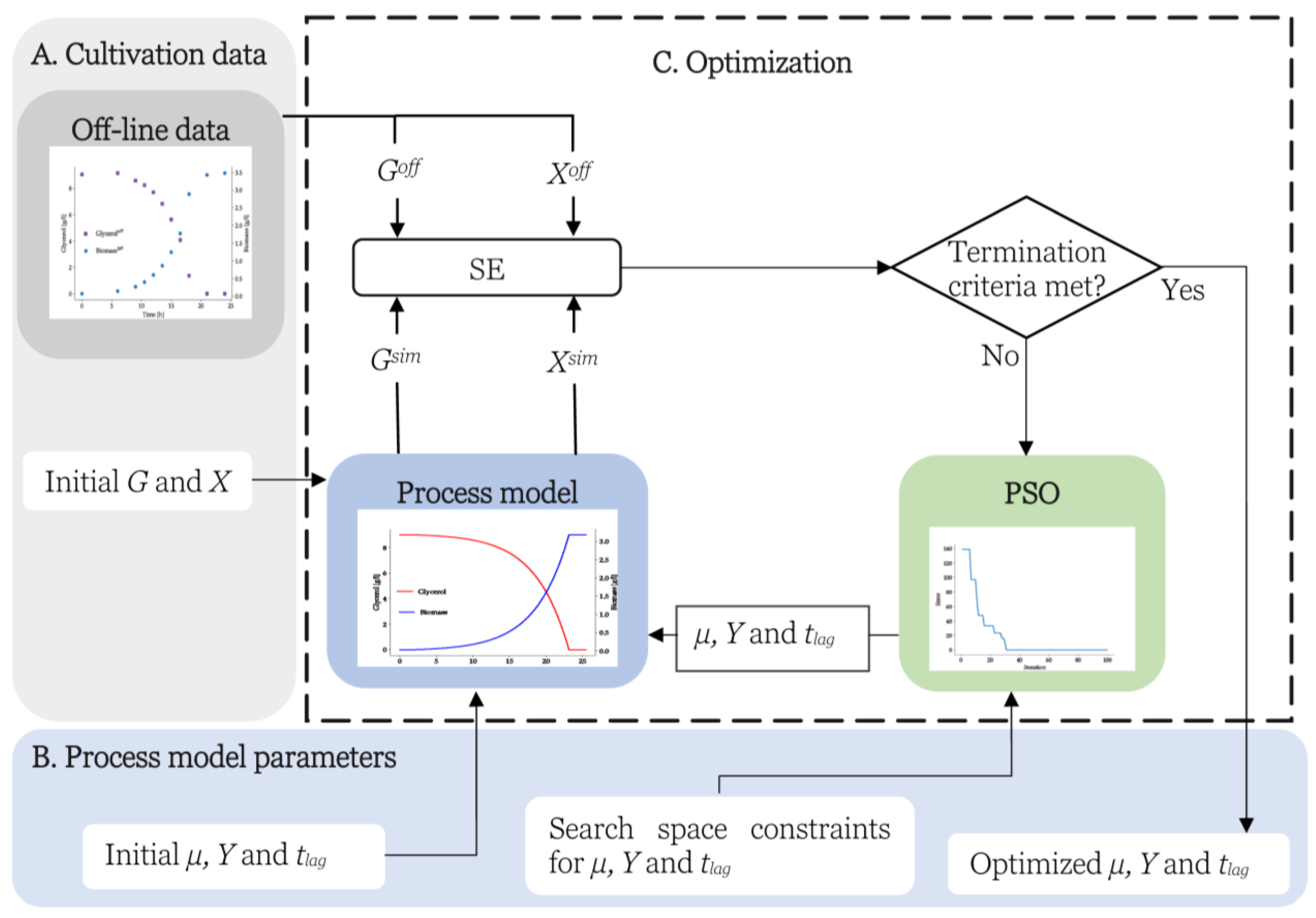
Figure 1 shows the classical approach to optimizing the process parameters using offline data and the mathematical process model. It starts with the initial concentration of glycerol (G) and biomass (X), and a random initial set of process parameters: µ, Y, and t_lag within the search space to calculate the simulated values for G and X over the time of cultivation. With the simulated and offline data, the fitness of the process parameters is calculated.

The higher the sum of error (SE), calculated by using Equation (5), the worse the quality of the proposed process parameters applied in the simulation is. A smaller SE indicates the given process parameters lead to the simulated values that are closer to the offline measurements. The optimization (Figure 1, section C, enclosed with the dashed line) is performed iteratively with the optimizer until a termination criterion is met. In every iteration, the optimizer proposes (most likely) a new combination of process parameters and repeats the evaluation procedure.

The process parameters for which the sum of error is the minimum are presented as optimized process parameters for that cultivation. If the cultivation conditions are kept constant, it is expected that despite the variation in initial G and X, the deviation in optimized process parameters between cultivations should be minimal. By using the mathematical process model with optimized process parameters and the initial conditions of any cultivation being plugged in, the state of the variables can be estimated at any measurement point.

2.6. Concept of Model-Based Calibration (MBC)

Optimized process parameters obtained based on offline measurement (Section 2.5) can be used to describe batch cultivation from simulated values of the process variables. In other words, by using the optimized process parameters and initial glycerol and biomass, the process state at any measurement point of new cultivation can be estimated. However, since the knowledge of earlier cultivations is employed for this estimation, it has no interaction with the real status of the new cultivation. To interact with a new cultivation system, a monitoring sensor is typically used, whose signals must be calibrated in order to build a model that predicts the process state online.

Calibration of a predictive model is the process of mapping raw sensor signals into actual values, such as the actual concentration of process variables. In conventional approaches, a large number of offline measurements are used as actual concentrations in this mapping procedure. For a given measurement point, the duplicates in offline data mostly do not show uniformity, and are considered to be random measurement errors or noise. In contrast, theoretical process models for bioprocesses specify the extent of interdependencies between variables through process parameters like microbial growth rate and substrate-to-biomass conversion rate. The estimated state of process variables can be derived from the theoretical process model once these process parameters have been acquired. In contrast to offline data, simulated concentrations stay consistent and coherent with continuous cultivation time as target variables against sensor signals, which makes the calibration or mapping procedure more accurate. Moreover, a sensor usually provides signals with a smaller time interval. The measurement interval in offline data is mostly high and distribution of them can be uneven throughout the cultivation time. It raises the possibility of having a wide range of cultivation times where the signals are not mapped with the corresponding actual concentrations. In practice, the linear interpolation of actual offline measurements is applied to have enough actual concentrations for calibrating the chemometric model, which influences the performance of the chemometric model [13]. By using a process model, in contrast, the simulated concentrations can be calculated with any smallest time interval, which allows for a high frequency in mapping against sensor signals.

The model-based calibration (MBC) replaces the laborious, costly, error-prone, and poorly mappable offline measurements with consistent, robust, and solidly mappable simulated data. In MBC, the process model is used to map 2D fluorescence spectra in calibrating a chemometric model. But a process model without known process parameters does not describe the specific cultivation and the standard approach to obtain them requires offline data. As an alternative, the MBC approach relies on the sensor signals, with an assumption that all the information of the cultivation state is captured by them either directly or indirectly. Therefore, the MBC approach finds the optimized process parameters and optimized chemometric model parameters at the same time.

Consider a case in MBC, where a set of process parameters is significantly different from what it should be, as these values are unknown at the beginning. By using these process parameters, the simulated glycerol and biomass concentrations over cultivation time can be calculated from the process model. These simulated data and the real fluorescence spectra are aligned with regard to cultivation time. The simulated data are considered as target values and fluorescence spectra as the independent variable to formulate chemometric models independently for glycerol and biomass. The data is separated into train and test sets and a chemometric model is calibrated using train spectra and simulated values. With this calibrated chemometric, the prediction of simulated test set values is performed. The difference between predicted simulated test values and simulated test values will be large because the features extracted from the real spectra do not correlate with the simulated values.

Therefore, a new set of process parameters has to be adapted in the process model in order to lead to simulation values which fit with the features extracted from spectra. Here the extracted features are always the same, as the same fluorescence spectra are used every time. However, the fitting quality in the chemometric model varies due to the change in simulated values, which depends on process model parameters. If a chemometric model predicts the test simulation values accurately, the corresponding process model parameters are optimal. Following this iterative approach, both a better predictive chemometric model and a process model that describes the observed cultivation are obtained at the same time. The following is the description of the MBC approach illustrated in Figure 2.

• The fluorescence spectra from the cultivations are prepared with respect to excitation and emission combinations to avoid scattered light. In addition, the initial glycerol (G) and biomass (X) concentrations with which the cultivations were conducted, are assumed to be known (Figure 2A).
• The constraints for the process parameters in the search space are defined. Based on literature and initial search space investigations, the range for µ, Y, and t_lag was set to 0.16–0.30 h⁻¹, 0.30–0.50 g_biomass/g_glycerol, and 2–6 h, respectively. Initially, a random combination of process parameters within their search space range is proposed (Figure 2B).
• By using the proposed process parameters and starting conditions in the mathematical process model, the cultivations are simulated (Figure 2C). The only difference in the simulation between the cultivations is their initial conditions, which leads to different simulated values at any point during the cultivation runtime.
• The intensity values of fluorescence spectra are scaled between 0 and 1 for each wavelength. Afterwards, principal component analysis (PCA) is applied to them, and only three principal components (PCs) are considered for the chemometric model. The concentrations of biomass and glycerol are predicted using the principal component regression (PCR) models in Equations (8) and (9), respectively.
  $$X_{pred}=p_{x0}+{(p}_{x1}\times {PC}_1)+{(p}_{x2}\times {PC}_2)+{(p}_{x3}\times {PC}_3)$$

  (8)

  $$G_{pred}=p_{g0}+{(p}_{g1}\times {PC}_1)+{(p}_{g2}\times {PC}_2)+{(p}_{g3}\times {PC}_3)$$

  (9)

  where $X_{pred}$ is the predicted biomass, $p_{x0},p_{x1},p_{x2}$ and $p_{x3}$ are the multilinear regression model parameters for biomass prediction, ${PC}_{1,}{PC}_2$ and ${PC}_3$ are the first, second and third principal components, respectively, $G_{pred}$ is the predicted glycerol concentration, and $p_{g0},p_{g1},p_{g2}$ and $p_{g3}$ are the multilinear regression model parameters for glycerol prediction.
• The simulated glycerol concentration and biomass are aligned with fluorescence spectra with respect to cultivation time. The obtained data is separated into two sets: calibration and test. Data from six cultivations are taken for calibration and the remaining cultivation is used to test the model. This way, one complete cultivation is always set aside for testing, and this is repeated until each cultivation is tested once (cross-validation). The calibration set consists of simulated glycerol, simulated biomass, and fluorescence spectra from six cultivations, whereas the test set has simulated glycerol, simulated biomass, and fluorescence spectra from one remaining cultivation.
• A multi-linear regression model is fitted using the calibration set and then tested using the test set. The calibration and test for biomass and glycerol are performed independently as follows.
  • For biomass, a chemometric model is fitted by using simulated calibration biomass, and PCs of calibration spectra. The chemometric model is tested by using PCs to get predicted biomass ($X_{pred}$). The error of prediction for biomass is calculated by using Equation (10).

    $$X_{RMSEP}=\left[\sqrt{\frac{\sum _{i=1}^n{\left(X_{pred,i}-X_{test,i}^{sim}\right)}^2}{n}}\right]\times \frac{100}{X_{range}}$$

    (10)

    where $X_{RMSEP}$ is the root mean squared error of prediction for biomass with regard to the range of biomass concentration ($X_{range}$), $i$ is the measurement index and $n$ is the total number of measurements.
  • Similarly, glycerol is predicted to show a trend that is comparable to simulated glycerol; however, this appeared to be shifted in terms of concentration level. The error in predicting glycerol is calculated using Equations (11) and (12). In the chemometric model, glycerol concentration is predicted based on the response shown by biomass. Due to the interaction between glycerol and biomass, chemometric models can capture the trend in glycerol but not the variation in the initial glycerol concentration. This barrier can be overcome by taking into account a correction measure, where all the predicted glycerol concentrations are adjusted by a certain amount, as illustrated in Equation (12). It is the difference between the predicted and actual initial glycerol concentrations of the test cultivation ($G_{pred,1}$−$G_0)$.

    $$G_{RMSEP}=\left[\sqrt{\frac{\sum _{i=1}^n{\left(G_{Cpred,i}-G_{test,i}^{sim}\right)}^2}{n}}\right]\times \frac{100}{G_{range}}$$

    (11)

    $$G_{Cpred,i}=G_{pred,i}+G_{pred,1}-G_0$$

    (12)

    where $G_{RMSEP}$ is the root mean squared error of prediction for glycerol with regard to the range of glycerol concentrations ($G_{range}$), $i$ is the measurement index, $n$ is the total number of measurements, $G_{Cpred,i}$ is the predicted glycerol concentration after shift correction, $G_{pred,1}$ is the first predicted glycerol concentration, and $G_0$ is the initial glycerol concentration of the test cultivation. The sum of errors (SE) is calculated by using Equation (13).

    $$SE=\sum _{c=1}^N(G_{RMSEP,c}+X_{RMSEP,c})$$

    (13)

    where $c$ is the index of cultivation that is used in the test set, $N$ is the total number of cultivations, $G_{RMSEP,c}$ and $X_{RMSEP,c}$ are the glycerol and biomass prediction errors, respectively, when cultivation $c$ was used for the test.
• SE is evaluated by PSO and starts the optimization procedure to minimize it. In order to improve the prediction error, PSO proposes a new combination of µ, Y, and t_lag within the search space.
• The procedure from step 3 to step 8 is repeated (Figure 2C) until a termination criterion for PSO is met. Finally, the optimized combination of µ, Y, and t_lag for which the multi-linear regression predicted the variables most accurately is saved. The optimal parameters for the theoretical process model and chemometric model are saved for further validation.

2.7. Improved Model-Based Calibration (IMBC)

In MBC, the predicted glycerol concentration is required to be corrected based on initial glycerol concentration (Equations (11) and (12)), which is a feasible approach since the initial concentration is known. However, in the case of biomass prediction, there is no such correction required. It implies that the fluorescence spectra carry uniform information on biomass regardless of its variation in initial concentrations in different cultivations. In contrast, spectra provide no hint of the variation in initial glycerol. Therefore, the prediction of glycerol concentration in this case is an indirect measurement and is predicted due to its correlation with biomass. A chemometric model can describe this correlation; however, it fails to include the exact level of glycerol the cultivation is initiated with. Theoretically, the correlation between biomass and glycerol is explicitly described by the process model.

An alternative approach of model-based calibration (IMBC) is used to improve glycerol prediction and avoid possible chaotic fluorescence intensities with regard to glycerol concentrations. In this approach, only biomass is predicted with a chemometric model based on 2D fluorescence spectra online. This predicted biomass is used in the theoretical process model to estimate glycerol concentration To obtain the estimated glycerol concentration from the process model in IMBC, the followings are required: initial glycerol and biomass concentrations, process model parameters (µ, Y, and t_lag), measurement time, and predicted biomass at the measurement time. The entire process can be completed online because the computation time is comparable to the time required by a chemometric model to predict glycerol. The procedure for IMBC is similar to the MBC presented in Section 2.6 with the minor modifications described in the following steps.

• Modification 1: The scaling of intensities of spectra is performed (in step 5) to have a better chemometric prediction for glycerol in MBC and is avoided in the IMBC.
• Modification 2: In the calibration of a chemometric model, the prediction and error calculation for glycerol (in steps 4 and 6b, respectively) are ignored. As a result, PSO evaluates (in step 7) only the sum of the errors from biomass ($X_{RMSEP}$) calculated in Equation (13).

The advantage of this approach is that the optimizer solely considers fitting simulated biomass with spectra and is not influenced by the glycerol prediction accuracy. If a certain combination of µ, Y, and t_lag leads to a simulated biomass that fits between the features in spectra, then the process model is most certainly able to estimate the glycerol concentration.

2.8. Validation of Model-Based Calibration

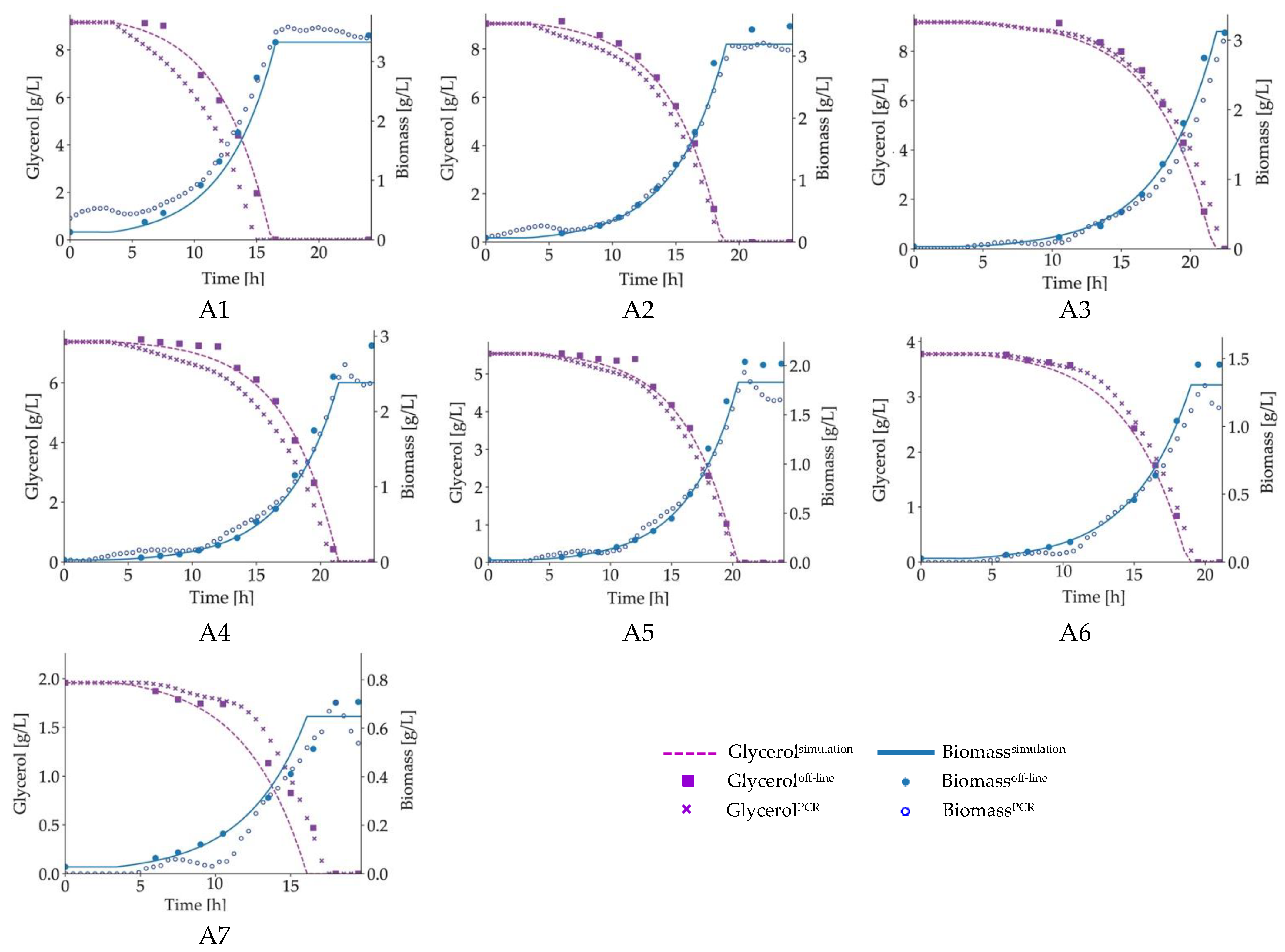
To validate whether the proposed model-based calibration approaches estimate the process variables precisely, the conventional procedure is followed. The offline measurements for the cultivations are not used in MBC and IMBC. Instead, whole calibration and cross-validation are performed by using 2D fluorescence spectra and simulated values for process variables. To determine the performance of these approaches, the offline measurements for the variables are used for comparison. The validation is performed in two ways: simulated values and predicted values from both MBC and IMBC.

3. Results

3.1. Initial Conditions of Cultivation

With various concentrations of the process variables, glycerol (1.96–9.17 g/L) and biomass (0.03–0.12 g/L), the initial conditions for each cultivation are displayed in

Table 1. Initial glycerol and biomass content of the cultivations.

Cultivations	Initial Glycerol [g/L]	Initial Biomass [g/L]
A1	9.16	0.12
A2	9.05	0.07
A3	9.17	0.03
A4	7.37	0.03
A5	5.54	0.03
A6	3.78	0.03
A7	1.96	0.03

. The orientation of the initial conditions covers variations in the biomass as well as glycerol concentration independently. Cultivations A1, A2, and A3 were carried out with variations in biomass concentration (0.03–0.12 g/L) and roughly the same concentration of glycerol (9.05–9.17 g/L). In contrast, the biomass concentration was constant (0.03 g/L) and glycerol concentration was varied (1.96–9.17 g/L) among cultivations A3, A4, A5, A6, and A7.

3.2. Optimization of Process Model Parameters

Before being used to calibrate a chemometric model, the theoretical process model must be representative of the behavior of the microorganism in the studied system, which is determined by three process parameters: µ, Y, and t_lag. The initial search space investigation follows the same methodology as MBC, where chemometric models are calibrated using fluorescence spectra and the theoretical process model. However, PSO optimized three process parameters in MBC, whereas optimization was not carried out in this case. Instead, one process parameter was held constant at a reasonable value based on previous knowledge, and the remaining two were varied within a certain range.

Figure 3 illustrates how the process parameters influence the calibration of a chemometric model by using the process model, with dark blue representing the lowest test error. Figure 3a shows the test error when t_lag was held constant at 4.6 h and µ and Y were varied. Below a µ value of 0.16 h⁻¹, for any Y value, the test error was lower, which does not reflect the actual state of H. polymorpha cultivations. A similar case was observed when Y was held constant at 0.34 g_biomass/g_glycerol and µ and t_lag were varied. Both cases (Figure 3a,b) had lower test errors in the range of 0.21–0.28 h⁻¹ for µ, pointing to a potential representative area for the cultivations under study. A range of 0.30–0.50 g_biomass/g_glycerol for Y was used for MBC and IMBC. Figure 3c shows the test error with varying Y and t_lag while µ was held constant at 0.27 h⁻¹, which indicates a reasonable range of 3–6 h for t_lag.

Table 2. Optimized process model parameters obtained in different approaches.

Approach	Source of Data	µ [h−1]	Y [gbiomass/gglycerol]	tlag [h]
Classical	Offline measurements	0.268	0.339	4.4
MBC	2D fluorescence spectra	0.261	0.334	3.9
IMBC	2D fluorescence spectra	0.247	0.317	3.8

shows the optimized process parameters obtained from three approaches using the theoretical process model. The key difference between the approaches is the data that was compared with simulated values: for the classical approach, it was offline measurements of glycerol and biomass whereas for the MBC and IMBC, it was chemometric model prediction values, with the latter only for biomass. There is no significant difference between the optimized values for µ and Y derived by the three methods; however, when only biomass prediction was taken into account (IMBC), optimized process parameters were slightly lower. The optimal t_lag value for the classical approach was 4.4 h, which was slightly higher than what was observed for the MBC and IMBC. This variation could be explained by the long time interval (6 h) between the two initial offline measurements, whereas fluorescence measurements have a measurement interval of 30 min. The optimized values for t_lag from MBC and IMBC, which both used data from spectra, were similar.

3.3. Validation of Model-Based Calibration

Each cultivation was left out of the calibration process once to validate the performance of model-based calibration approaches by using its data. The calibration approaches deliver optimized process parameters and chemometric models for glycerol and biomass prediction simultaneously. The validation was carried out in two ways: to validate if the optimized process parameters represent the left-out cultivation and to validate if the chemometric model can predict process variables from the fluorescence spectra of the left-out cultivation. As a result, the left-out cultivation was simulated with optimal process parameters and initial conditions and then compared to real offline measurements. Similarly, predicted glycerol and biomass concentrations from chemometric models were compared to offline measurements. The validation was repeated seven times to quantify the average root mean squared error (RMSE) across all cultivations, each time leaving out one different cultivation from the calibration.

Table 3. Validation of simulated values with offline measurements. The simulated glycerol and biomass were used to train the chemometric model and to perform the principal components regression (PCR); these were different for the approaches due to the variation in optimized process parameters.

Approach	Biomass RMSE		Glycerol RMSE
	[g/L]	[% Range]	[g/L]	[% Range]
Classical	0.10	3.0	0.22	2.4
MBC	0.09	2.6	0.29	3.1
IMBC	0.13	3.6	0.22	2.4

compares the simulated biomass and glycerol concentrations to offline measurements. These simulated values are obtained from the process model by using optimized process parameters with all errors ≤3.6% of the concentration range. The results reflect that the simulated process variables calculated based on MBC and IMBC approaches are close to the real offline measurements despite no offline measurements being used at any stage of analysis. IMBC lowered the error for simulated glycerol (2.4%), however, the error for simulated biomass is increased compared to MBC. Nevertheless, the main goal is to use these simulated values in place of offline measurements as target variables in the chemometric model training process against 2D fluorescence signals as independent variables.

Table 4. Cross-validation of predicted glycerol and biomass concentrations with offline measurements. The prediction was performed by the chemometric model (PCR) trained with simulated glycerol and biomass concentrations. In the case of IMBC, the glycerol concentration was indirectly predicted from the process model by using the predicted biomass.

Approach	Biomass RMSE		Glycerol RMSE
	[g/L]	[% Range]	[g/L]	[% Range]
Classical	0.20	5.7	0.82	8.9
MBC	0.20	5.7	0.79	8.6
IMBC	0.16	4.7	0.48	5.2

presents the validation results for chemometric predictions. The chemometric validation error for biomass showed the same level of error (5.7%) for classical and MBC approaches while IMBC improved it significantly (4.7%). In contrast, glycerol showed a high range of error across different approaches with the classical approach being the worst (8.9%), followed by MBC with no substantial improvement. In contrast, IMBC showed significant improvement in the prediction of glycerol concentration with only a 5.2% error. The results reveal that the prediction results from the classical approach and the MBC are apparently very similar. It confirms that a model-based calibration approach is equally efficient as the classical approach. IMBC took advantage of better prediction of biomass from fluorescence to increase the prediction accuracy for both biomass and glycerol with the lowest prediction errors of 5.2% and 4.7% respectively.

Figure 4 shows the predicted, simulated values validated with offline measurements for the cultivations using MBC. In this approach, the simulated values are aligned with the offline measurements and the prediction of biomass by a principal components regression model (Biomass^PCR) followed the trend as the error was 5.7%. However, it is clear that the lower concentrations of glycerol (<2 g/L) were not predicted accurately by the principal components regression model (Glycerol^PCR) in all cases and therefore had higher validation error (8.6%).

Figure 5 presents the validation results for the IMBC, where the prediction of biomass (Biomass^PCR) was only performed using a chemometric model based on 2D fluorescence spectra. The predicted biomass showed a better fit with both offline and simulated biomass. The predicted biomass concentration was used as an input in the process model to obtain the actual glycerol concentration. Figure 5 shows that the approach is effective in predicting both higher and lower concentrations of glycerol and therefore had a lower prediction error (5.2%).

4. Discussion

For all calibration approaches, the difference between the simulated and the real offline measurements for glycerol and biomass concentrations was ≤3.6% (Table 3). It shows that small variations in the process parameters do not significantly affect the simulated values used to represent the system. However, the chemometric prediction results for biomass are only good when the same simulated values are used to train the chemometric models (classical and MBC). Glycerol is said to rely on the fluorescence of biomass because it does not present on its own. Since glycerol and biomass concentrations in the studied system have a high correlation, 2D fluorescence can be utilized to predict glycerol concentration indirectly through the fluorescence displayed by the biomass. According to Paquet-Durand et al. [18], this indirect calculation causes glycerol’s chemometric prediction error to be larger than that of the biomass. Since only sensor signals are used in model-based calibration approaches to extract information from an actual biosystem, it can be argued that the more process variables that exhibit a response in signals, the better.

In order to calibrate a chemometric model for the growth of S. cerevisiae, Solle et al. [19] used MBC with test errors from biomass, ethanol, and glucose in calibration. Yousefi-Darani et al. [27], in contrast, used MBC to exclusively predict ethanol concentration in S. cerevisiae cultivations from ethanol-sensitive sensor array signals. Only taking the ethanol prediction error into account during calibration led to higher ethanol prediction accuracy. Paquet-Durand et al. [18] calibrated PLS regression models for H. polymorpha using biomass and glycerol error, which is the same method used for MBC in the present study. According to the study [18], glycerol had a relatively high prediction error (9.8%) compared with biomass (4.7%), which is consistent with the findings of the current study utilizing the MBC technique (8.6% and 5.7%, respectively).

Instead of relying on the inferential prediction of glycerol from fluorescence signals, IMBC made use of the interaction between variables as a system defined by a mathematical process model. The results show that the prediction of glycerol and biomass were both improved, with validation errors of 5.2% and 4.7%, respectively. The reason is that the process parameters are optimized from fluorescence spectra in MBC and IMBC. Since glycerol does not show any fluorescence, only the error for biomass was used to find the best combination of process parameters and to calibrate a chemometric model in the IMBC. Similarly, only biomass was predicted during the prediction stage using a chemometric model based on fluorescence signals, which delivers better prediction accuracy. The glycerol concentration was computed with a similar degree of accuracy using the theoretical relation indicated by the mathematical process model.

5. Conclusions

The current study’s objective was to define and implement alternative calibration techniques for chemometric models in order to eliminate the need for a substantial number of offline measurements. The optimized process parameters were obtained directly from 2D fluorescence spectra by exploiting a mathematical process model that explicitly describes the cultivation system of H. polymorpha. In order to train the chemometric models from spectra simultaneously, the simulated values were computed by plugging in the optimum process parameters. Offline measurements were not employed at any stage in the calibration procedure.

A classical approach using offline measurements of glycerol and biomass was also applied to verify the performance of model-based calibration (MBC). The optimized process parameters were obtained by fitting offline measurements against simulated data. The best-fitted simulated data was then used to calibrate chemometric models and predict the process variables from 2D fluorescence spectra. To determine the optimized process parameters and chemometric models for glycerol and biomass concentrations in MBC, 2D fluorescence spectra were used. Only biomass was considered during calibration and prediction in the IMBC, which differs from MBC.

The findings indicate that the classical approach had the largest prediction errors for glycerol (8.9%) and biomass (5.7%), which is similar to that of MBC (8.6% and 5.7%, respectively). With prediction errors of 5.2% for glycerol and 4.7% for biomass, IMBC significantly improved the prediction accuracy while at the same time requiring no offline measurements for training. The cross-validation results demonstrate that model-based calibration approaches can be applied to online state estimation for H. polymorpha cultivation.