1. Introduction
Beer, wine, cider, and other alcoholic beverages have been part of our civilization for thousands of years even before their scientific underpinnings were fully understood. It was only in the 19th century that Louis Pasteur was able to prove that yeast is an essential driver in alcoholic fermentation [
1]. Ethanol production is primarily a consequence of anaerobic conditions created by rapid yeast growth along with increasing nutrient and sugar limitations; this eventually leads to active fermentation metabolism and, finally, increased ethanol production [
2]. In most instances, yeast strains currently used in industrial fermentation processes at breweries and wineries belong to the
Saccharomyces cerevisiae (
S. cerevisiae) species. This yeast species is highly efficient in the alcoholic fermentation processes due to its ability to convert sugar into ethanol, its high fermentation power, and adaptability to changing conditions during biotechnological use [
3]. After many years of classical industrial production, where process parameters are monitored offline and require sampling as well as time-consuming analytical methods, the industry is now rapidly moving toward digital transformation. Automated and digitalized processes allow for a fully controlled, flexible, and highly efficient production process that ensures high-quality products. This not only results in a standardized and cost-efficient production but also reduces process-associated risks.
Increasingly, inline process analytical technologies (PATs) are applied for real-time and in situ monitoring of parameters, such as pH, temperature, and dissolved oxygen. Thereby, large amounts of data are collected that feed into the mathematical modeling of processes, their prediction, and control. In high-value fields like biopharmaceutical production, PAT is gradually replacing traditional standard physical sensors within reactors [
4], suggesting its potential use in other biotechnological processes, such as alcoholic fermentation.
At present, the production of alcoholic beverages requires monitoring yeast viability, cell count, and growth behavior in order to ensure a controlled, constant, and reproducible fermentation process [
5]. State-of-the-art technologies to determine the number of viable and non-viable cells include classical colony counting to determine the number of viable cells. Non-viable cells are often determined by staining techniques using dyes like methylene blue and slide culture procedures [
6,
7,
8]. However, these microbiological techniques are time-consuming and error-prone (e.g., they suffer from false positive results due to long exposure times and subjective evaluations). Hence, there is a strong need for a fast, non-invasive, and non-biased method to evaluate yeast cell viability during fermentation processes to ensure high-quality products and prevent microbiological contamination.
Spectroscopical methods like Raman spectroscopy (RS) are very powerful tools for the identification, quantification, and monitoring of metabolites or materials amenable to non-invasive, real-time, and inline measurements, while avoiding sample preparation. For example, non-invasive inline RS measurements are already being utilized in feedback control systems to improve ethanol production, which enables the real-time quantitative analysis of glucose and ethanol during
S. cerevisiae fermentation [
9,
10,
11]. Beyond that, RS has the potential to serve as a powerful tool to identify, quantify, and monitor microbes, representing a valuable technology for inline measurements of fermentation processes [
12]. Namely, RS provides detailed information on the molecular level, a “fingerprint” that enables the discrimination of closely related bacteria or the identification of bacterial contaminants in food products based on the analysis of Raman spectral differences [
13,
14,
15,
16,
17,
18]. Several studies have been performed to evaluate the application of Raman imaging, e.g., for food quality and safety control [
19,
20,
21]. Yet, while non-destructive and highly precise [
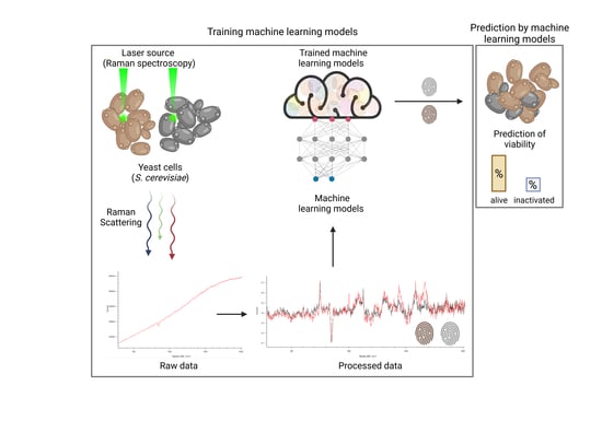
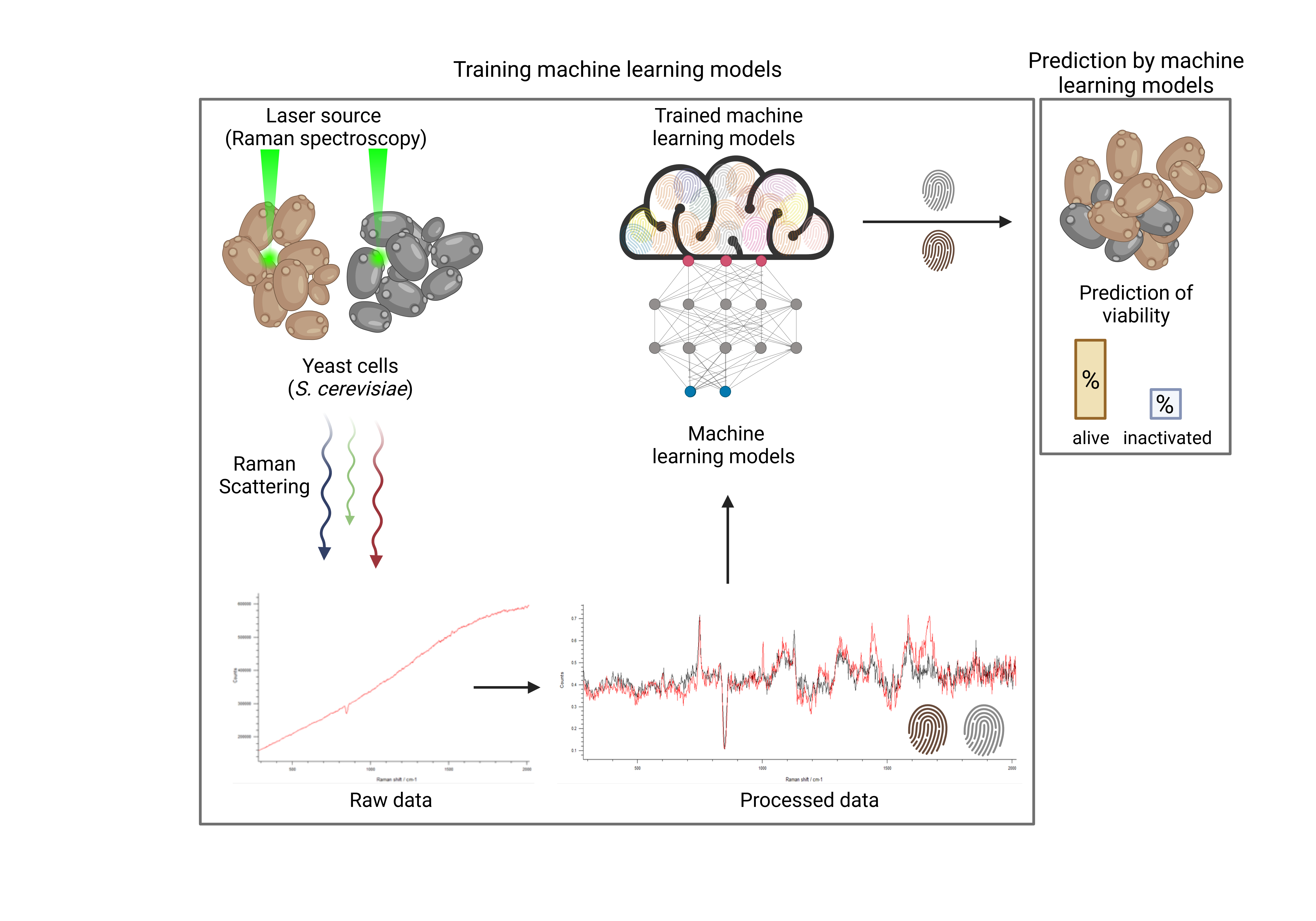
18], limited data exist for Raman-based methods for monitoring yeast in biotechnological brewing processes. The present work, therefore, focuses on the initial evaluation of the effectiveness of RS combined with predictive machine learning (ML) models for prospective real-time monitoring and determination of yeast viability in biotechnological processes.
In this study, we obtained spectroscopic datasets of viable and heat-inactivated yeast cells of different species and cultured them in different media to train ML models. Six ML approaches were considered and their viability prediction performances were compared in terms of the balanced accuracy (i.e., normalized values between zero and one, with the latter representing 100% prediction accuracy). Furthermore, the influence of artificially added noise on prediction accuracy was investigated to estimate the impact of imperfections in actual ex vitro measurements.
2. Materials and Methods
2.1. Organisms and Growth Media
Two yeast strains used in this study, S. cerevisiae (ATCC 18824) and Dekkera bruxellensis (Dekkera bruxellensis (D. bruxellensis)), formerly labeled as Brettanomyces bruxellensis, were purchased from ATCC (Manassas, VA, USA) and White Labs Brewing Co. (San Diego, CA, USA), respectively. Yeast extract peptone dextrose (YPD) culture medium (20 g L peptone, 10 g L yeast extract, and 20 g L glucose) were used for yeast cultivation. Yeast culture was inoculated to a ratio of 1:500 in YPD medium followed by incubation at 32 °C and 170 rpm for 20 h or 72 h, respectively. These timespans were chosen due to laboratory practicability and monitoring over time. For RS analysis, additional media (commercially available beer and apple juice) were purchased and sterile-filtered (0.22 μm pore size). Ultrapure HO (Milli-Q) was used as the negative control.
2.2. Sample Preparation for Raman Spectroscopy
For sample preparation, grown cultures of S. cerevisiae and D. bruxellensis were pelleted by centrifugation (5000× g, 5 min), washed with HO, and adjusted to an optical density (OD600) of 10 to ensure a constant amount of cells in each sample. For S. cerevisiae, 1 mL of culture was incubated at 72 °C for 10 min followed by incubation on ice for one minute (referred to as “heat-inactivated” in the following sections). Additionally, 1 mL of each sample was kept at 32 °C, followed by incubation on ice for one minute (referred to as “viable” in the following sections). For different media tested, S. cerevisiae cultures grown in YPD were mixed with either sterile-filtered beer, apple juice, or water, and adjusted to an optical density (OD600) of 10. For mixed samples, yeast cultures of S. cerevisiae and D. bruxellensis (considered as artificial contamination) were adjusted to an OD600 value of 10 in HO followed by mixtures in different ratios, as stated in the following section. From each sample produced, 20 L were applied to lime soda slides (Carl Roth), followed by air fixation for spectroscopic analysis.
2.3. Raman Spectroscopy
The RS analysis of samples was performed using an inViaTM Quontor Raman spectroscope (Renishaw plc, Wotton-under-Edge, United Kingdom). Raman spectra of 50 to 60 randomly selected yeast cells of several sections in each sample were obtained using a dry objective (0.85 NA) with a 45 W 532 nm laser adjusted to an intensity of 10% and 1 s exposure. To reduce background noise, each measurement was accumulated ten times for each cell. Raw data acquisition was obtained in a spectral detection range of 283 cm to 2016 cm. The scattered radiation was passed through a notch filter, focused onto a monochromator with 1800 lines mm grating, and detected by a Peltier-cooled CCD camera (1024 pixel × 256-pixel sensor).
2.4. Dataset Composition
Acquired datasets of
S. cerevisiae were categorized into 10 different groups, depending on the condition (viable, heat-inactivated), background media (YPD, beer, apple, juice and H
O) and different time points of the measurements (20 h and 72 h) for the analysis, as listed in
Table 1 and
Table 2. In addition, two mixed-sample models were produced to simulate more realistic conditions, as listed in
Table 3. Mixed samples were composed as follows: The first set of samples consisted of 33% viable and 33% heat-inactivated
S. cerevisiae cells mixed with 33% viable
D. bruxellensis culture for equal distribution. The second set of samples consisted of 75% viable and 20% heat-inactivated
S. cerevisiae culture mixed with 5% viable
D. bruxellensis culture. Since
D. bruxellensis shows, to some extent, similarity to
S. cerevisiae on the sequence level [
22], it is suitable to demonstrate the contamination of a sample with a related yeast strain. With respect to
S. cerevisiae, the second mixture is mostly heat-inactivated, whereas the first mixture contains the same ratio of viable and heat-inactivated cells. In the scope of this work, we consider the first mixture as viable and the second as heat-inactivated.
3. Machine Learning Methods
As presented in
Table 1,
Table 2 and
Table 3, we considered six datasets, which were compiled from the RS experiments:
H2O,
Apple,
Beer,
YPD-20,
YPD-72,
Mix. Additionally, we combined all datasets into a joint dataset
All. Each dataset consists of spectroscopic data of yeast samples, which are either viable or inactivated by heat. For the
Mix dataset, we considered the second mixture with 708 measurements as viable (since the majority of
S. cerevisiae in the mixture is viable) and the first mixture with 1004 measurements as heat-inactivated.
To summarize, the practically relevant goal was to identify the binary viability of yeast (viable/heat-inactivated) from the spectroscopic data by means of pattern recognition: a well-defined classification problem. That is, the ML task was to assign a class label—either viable or heat-inactivated—for Raman spectra obtained from each single yeast cell measured in the samples. In other words, we searched for an algorithm that allows the mapping
such that an RS of a yeast sample is sufficient for identifying its viability.
In the following, we first describe the data-processing pipeline that has allowed us to cast the raw measurement data into a suitable form. Since we only performed in vitro measurements, we also included a noising process in our pipeline that allowed us to induce artificial noise to emulate a less ideal (i.e., ex vitro) scenario. In other words, we considered the artificially induced noise as the presumed influence of potential ex vitro measurements on the data in contrast to data from the actually performed in vitro measurements. Our data-processing pipeline fully defines our classification problem. Subsequently, we briefly describe the ML models that we use to solve this problem.
3.1. Data Processing Pipeline
Each raw dataset consists of N data points of the form , which are composed of a vector of wave numbers and a vector of corresponding intensities for . Furthermore, each dataset is associated with a yeast viability label , where 1 represents viable and 0 represents heat-inactivated yeast. These labels constitute the ground truth. The wave numbers were measured in the range of 283 cm to 2016 cm, whereas the corresponding intensities were measured in arbitrary detector units.
First, we performed a preprocessing of the data to transform it into a unified form that is suitable for ML applications. For each data point n, five preprocessing steps were used. We
Interpolated the intensities uniformly, such that they spanned the same wavelength domain.
Rescaled the intensities to the unit interval.
Fixed a systematic error in the measurement results by linear interpolation for wavelengths in the range of 830.437 cm to 864.667 cm. This systematic error is a direct result of the hardware used in the experimental setup.
Performed a baseline correction.
Performed a standardization of the intensities.
To simplify the notation, we omit all measurement units in the following. A detailed description and formal definition of the data-processing pipeline can be found in
Appendix A. For data point
n, the resulting vector of wave numbers and the corresponding intensity vector are denoted by
and
, respectively. In
Appendix B, we show the mean
and standard deviation
of each preprocessed dataset, divided into data for
(viable) and
(heat-inactivated) to emphasize the differences.
To simulate the effects of ex vitro measurements, we also considered data, which have been perturbed by artificially generated noise. As formally described in
Appendix A, the absolute noise level is controlled by a parameter
that can be chosen at will. The resulting intensity vector for data point
n is denoted by
. We performed a perturbation for all datasets for different values of
. The signal-to-noise ratio decreases as the perturbation
increases, as visualized in
Appendix B.
3.2. Classification Models
Formally, our goal was to predict the yeast viability
(viable or heat-inactivated) from the measured Raman spectrum
. This corresponds to the classification problem
as a formal representation of (1) mapping from features
to class labels
y. For this purpose, we propose five well-known ML approaches to solve this problem and comparatively discuss their performances.
These approaches were chosen to represent conceptually different strategies [
23,
24]. The first three approaches constitute different kinds of ensemble methods based on a collection of decision trees. An ensemble method combines a set of models with the goal of creating a new model with better performance than the individual models from the set. In our case, the individual models are decision trees. Each decision tree consists of a set of binary decisions (i.e., inequalities for single features) that are traversed in a tree-like fashion to predict class labels. The fourth approach is a variant of Bayesian inference, whereas the last two approaches are established standard methods based on the optimization of a loss function. Specifically, we consider the following six ML approaches:
Random forest classifier (RF) [
25]. An RF is an ensemble method based on decision trees, where each tree is trained on a random subset of the training dataset to enable diversification and reduce overfitting. This ensemble strategy is also known as “bagging”. The average of all decision tree predictions decides the resulting class label prediction for the random forest classifier.
Gradient boosting classifier (GB) [
26]. A GB is an ensemble method based on decision trees similar to an RF. However, instead of relying on randomized diversification, an ensemble strategy known as “boosting” is used. This strategy iteratively adds decision trees to the ensemble with the goal of improving the resulting prediction. This strategy can lead to better overall models but is more vulnerable to overfitting than an RF.
EXtreme Gradient Boosting classifier (XGB) [
27]. An XGB is an extension of a GB that includes various improvements with the goal of pushing gradient boosting to its limits. However, it is not guaranteed that XGB generally performs better than GB; therefore, we consider both approaches.
Gaussian process classifier (GPC) [
28]. A GPC is based on Bayesian inference, where a Gaussian process is used as a prior probability distribution. Such a Gaussian process is defined by a collection of random variables with a joint Gaussian distribution. Due to the Bayesian premise, the resulting model allows to assign an uncertainty to each class label prediction.
Support vector machine classifier (SVM) [
29,
30]. An SVM is determined by the solution of an optimization problem with the goal of finding a hyperplane in the feature space that best distinguishes the class labels. We use a (radial basis function) kernel machine that maps the feature into a higher-dimensional space to enable non-linear separation.
Neural network (NN) [
31]. A NN consists of a set of layers, each of which maps its input to an output based on a predefined functional dependency that is determined by a set of trainable parameters. The features constitute the input for the first layer and the output of the last layer determines the class label predictions. A gradient-based learning algorithm is used to optimize a loss function with the goal of choosing trainable parameters that achieve the best class label prediction for the training data. Neural networks are highly generic models that can be customized in many ways due to their modular structure. However, this customization capability is, at the same time, a challenge, as good architecture (i.e., design of layers) is not always obvious. For this reason, we use a neural architecture search (NAS) algorithm to also optimize the architecture of the neural network in addition to its parameters. Specifically, we consider architectures with and without one-dimensional convolutions that are typically used for data in the form of time series.
In
Appendix C, we specify the details and parameters of the presented models. For further reading, we refer to the cited references and references therein.
4. Results
In the current section, we present our numerical results for the yeast viability classification task. We start with a proof of concept and consider the basic in vitro scenario for yeast in water, which only involves the H2O dataset without artificial noise. Subsequently, we show how well the proposed ML approaches perform in other media. Next, we study the effect of mixtures of different yeast strains representing artificial contamination within a sample and its influence on the model performances. Finally, we present the effect of artificially imposed noise within our data-processing pipeline on the model performances using different media and mixtures.
4.1. Proof of Concept: Predicting Yeast Viability
As a first study, we considered the
H2O dataset as described in
Section 3, which is based on Raman spectra of
S. cerevisiae in water (control) and free of artificial background noise. In total, 722 Raman spectra were available for training and analysis purposes according to
Table 1. Based on this data, we evaluated how six different ML approaches performed on the classification problem from (2). For each approach, we trained on the preprocessed
H2O dataset with a 10-fold cross-validation setup. That is, we split the dataset into 10 parts (further referred to as “chunks”) of approximately the same size. Here, and in the following, we used a so-called “stratified” approach, such that approximately the same ratio of viable and heat-inactivated samples are present in each split. The models were then trained independently on nine out of the 10 chunks, leaving one chunk remaining for testing purposes. Consequently, each data point was used nine times as training data and once as test data for each model. The ten training runs resulted in ten classifiers for each ML approach.
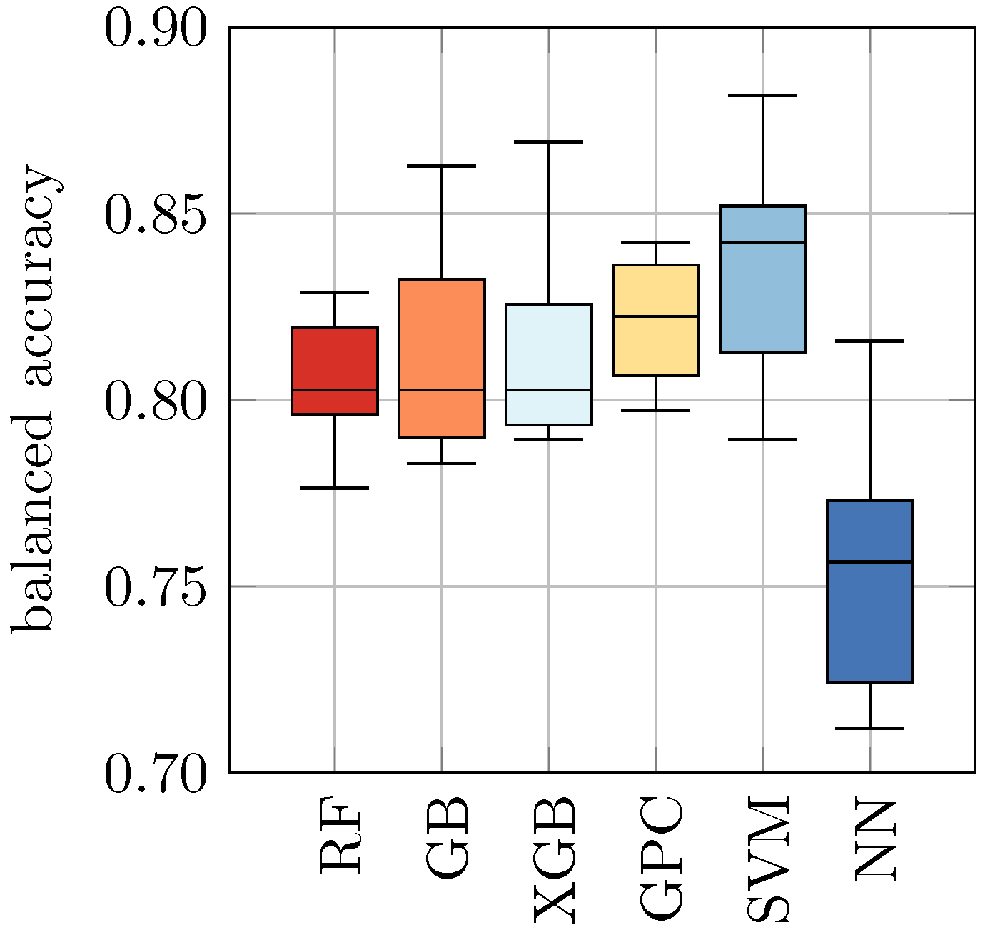
In
Table 4 and
Figure 1, we present the
balanced accuracies of all ML approaches, evaluated on the test dataset. The balanced accuracy represents the fraction of correct predictions over all samples weighted by the respective amount of samples for each class, such that class imbalances are accounted for [
32]. This compensates for the fact that we have slightly fewer heat-inactivated samples than viable samples in the dataset. The balanced accuracy can attain values between 0 (worst, i.e., all predictions are wrong) and 1 (best, i.e., all predictions are correct), where a value of 0.5 is the score of a random guess. For each ML approach, we obtained ten balanced accuracies based on the ten different data splits and could, therefore, determine the corresponding means and standard deviations.
As listed in
Table 4, we found in our study that the balanced accuracy ranges from 0.76 ± 0.03 for NN to 0.84 ± 0.03 for SVM. The remaining models achieved a balanced accuracy of 0.82 ± 0.03 and 0.81 ± 0.02, respectively.
4.2. Yeast Viability in Different Media
In the next step, we evaluated the performance of the models trained on the
H2O dataset predicting yeast viability in other media, i.e., the
Apple,
Beer,
YPD-20, and
YPD-72 datasets. As listed in
Table 2, these datasets originate from
S. cerevisiae in YPD, beer, and apple juice, as viable or heat-inactivated samples, respectively. Additionally, for YPD, two different time points (20 and 72 h) are used. Our ML models of interest are all classifiers that were trained on
S. cerevisiae in H
O (control) with 10-fold cross-validation, as presented in
Section 4.1. That is, we have ten trained classifiers for each ML approach.
As a first numerical experiment, we used the datasets
Apple,
Beer,
YPD-20, and
YPD-72 as inputs for each of these trained models and predicted the class labels (without retraining), i.e., we used the models that were trained only with Raman spectra of yeast in water to predict the viability of yeast in other media. Based on these predictions, we evaluated the balanced accuracy. The results are presented in
Table 5 (a) and
Figure 2. We found that previously trained classifiers showed a rather poor performance on yeast in other media, ranging from 0.49 ± 0.00 for RF, GB, XGB, and SVM on
YPD-20 to 0.60 ± 0.01 for SVM on
Apple. We recall that a balanced accuracy of 0.5 corresponds to a random guess. Hence, these results indicate that the application of ML models that have only been trained on control samples (i.e.,
S. cerevisiae in water) are not suitable for the discrimination of viable and heat-inactivated yeast cells in other media. Consequently, it seems mandatory for practical applications to train individual ML models for each background medium of interest.
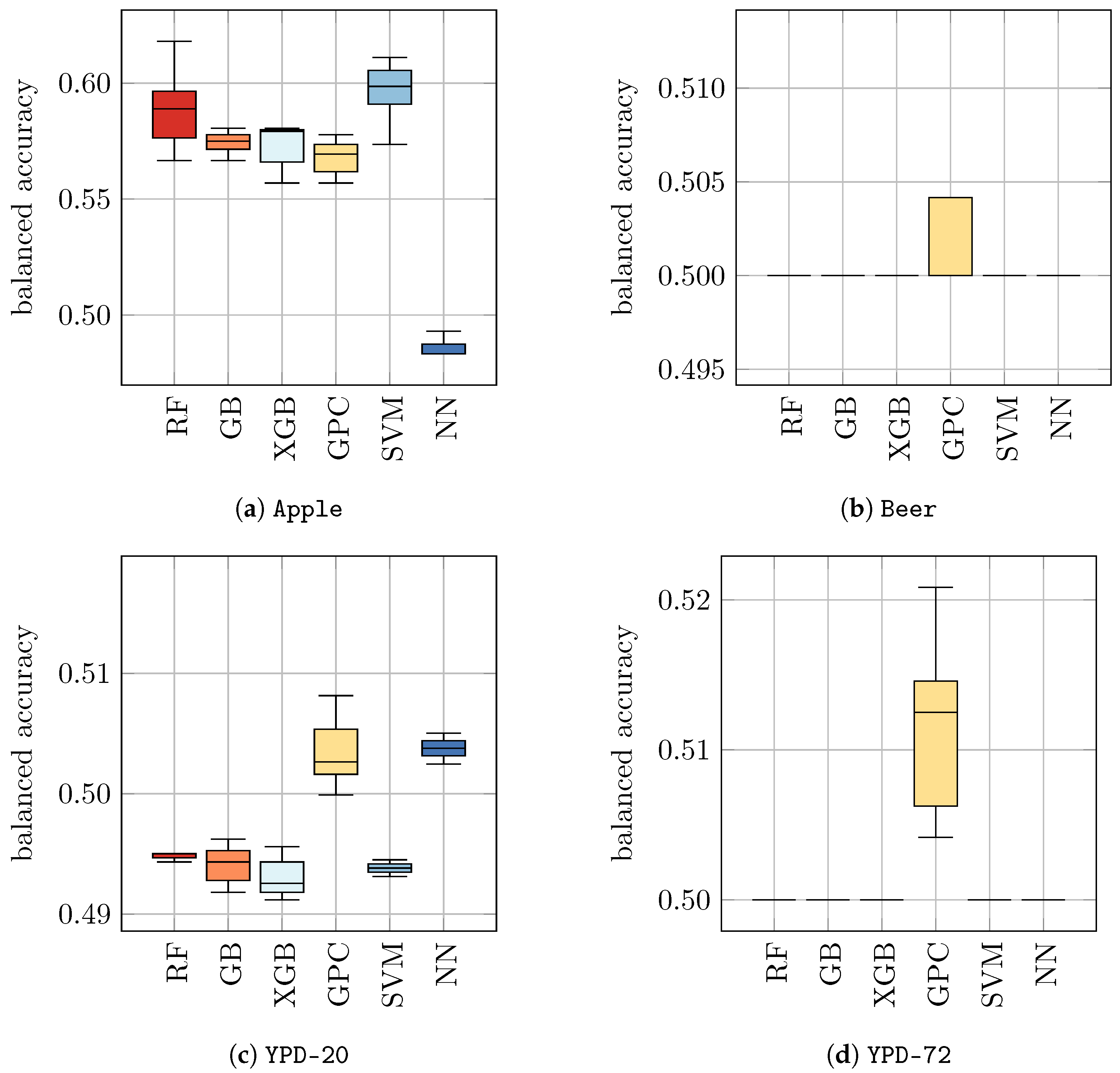
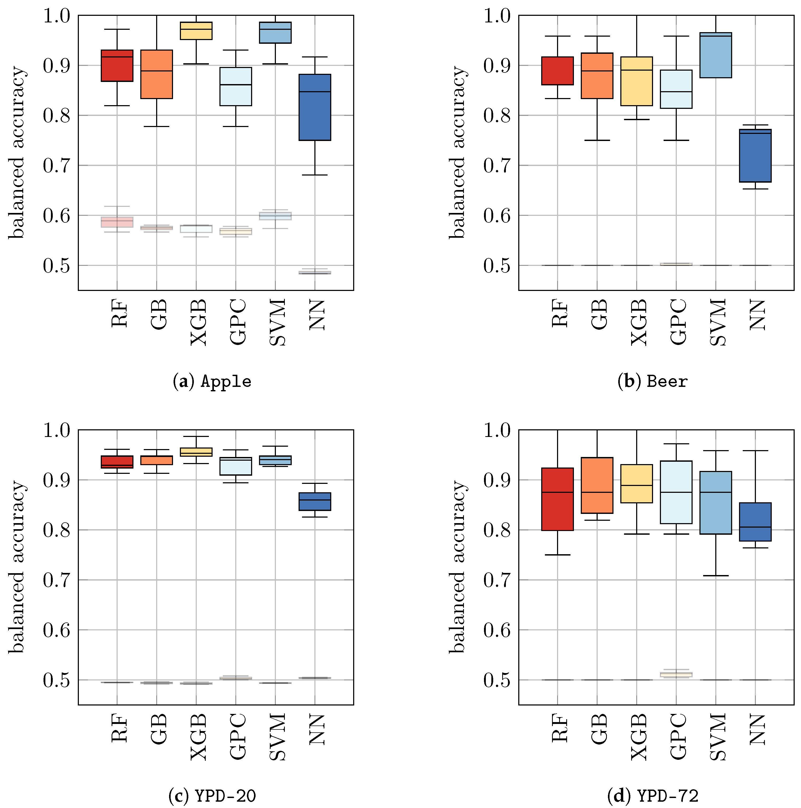
As a consequence of these findings, we trained new models on each dataset separately, following the approach detailed in
Section 4.1. That is, we considered the same four datasets as before (
Apple,
Beer,
YPD-20, and
YPD-72) and trained ten classifiers on each dataset for each ML approach using 10-fold cross-validation. With this approach, we checked if the predictive performance could be increased with different data. The results are presented in
Table 5 (b) and
Figure 3. Indeed, we found that for all datasets tested in this approach, the performances of ML models significantly improved compared to models that were only trained on
H2O. The resulting balanced accuracy ranged from 0.73 ± 0.05 for NN on
Beer to 0.97 ± 0.03 for GPC and SVM on
Apple. To enable a better comparison, we show the balanced accuracies of classifiers trained on datasets with yeast in media as solid boxplots in
Figure 3, whereas the classifiers from
Figure 2 (that were trained on
H2O) are displayed opaquely.
4.3. Viability of Mixed Strains
The previously obtained results raise the question as to whether ML approaches are also able to discriminate viable from heat-inactivated
S. cerevisiae if other yeast strains are present in the sample. To study this question, cultures of
D. bruxellensis—which is known as an undesired organism in wine production—were cultivated in YPD, followed by resuspension in water. Samples containing additional amounts of viable and heat-inactivated
S. cerevisiae lead to the dataset
Mix, as listed in
Table 3.
In analogy to
Section 4.2, we pursued two approaches. First, we used the classifiers that were trained on
H2O and use
Mix as input. Based on the predictions, we evaluated the balanced accuracy to determine if the classification also works for mixtures without having appropriate data in the training dataset. Second, we directly trained classifiers on
Mix using 10-fold cross-validation in analogy to
Section 4.1 and evaluated the balanced accuracy. The results are presented in
Table 6 and
Figure 4. In both cases, ML approaches led to a relatively low balanced accuracy for the mixed samples. In the first case, the balanced accuracy ranged from 0.47 ± 0.01 for NN to 0.50 ± 0.01 for RF, whereas in the second case, it ranged from 0.54 ± 0.04 for NN to 0.56 ± 0.03 for GPC.
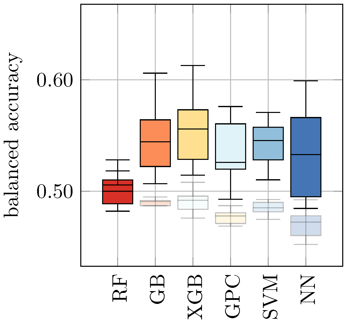
As an alternative approach, we combined all datasets from this study into a new dataset:
All. Again, in analogy to
Section 4.1, we trained and evaluated all ML approaches on this dataset using 10-fold cross-validation. The results are shown in
Table 7 and
Figure 5. We found that this approach revealed slightly increased balanced accuracy in comparison to the results from
Table 6 and
Figure 4, but a decreased score in comparison to the results from
Table 5 (b) and
Figure 3. The balanced accuracy ranges from 0.70 ± 0.02 for NN to 0.73 ± 0.01 for GPC and 0.73 ± 0.02 for SVM.
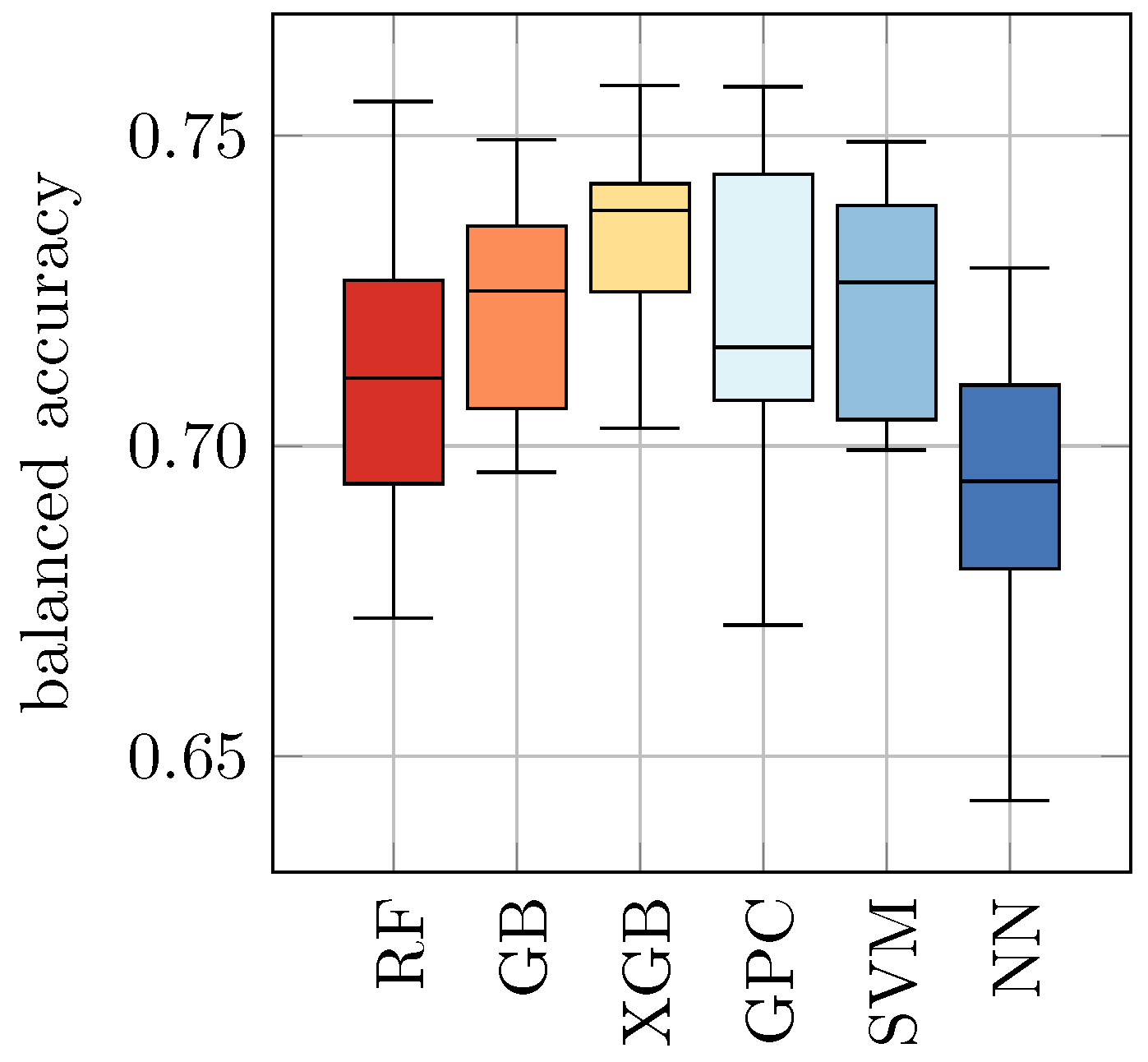
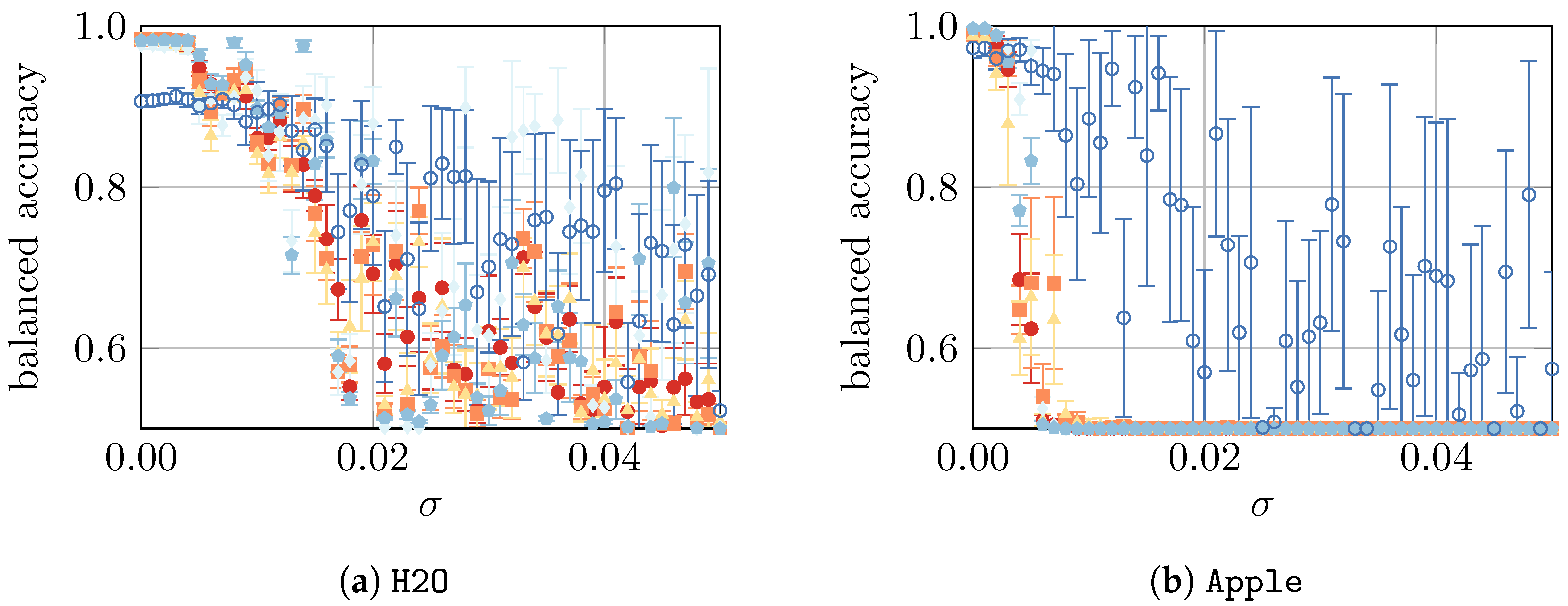
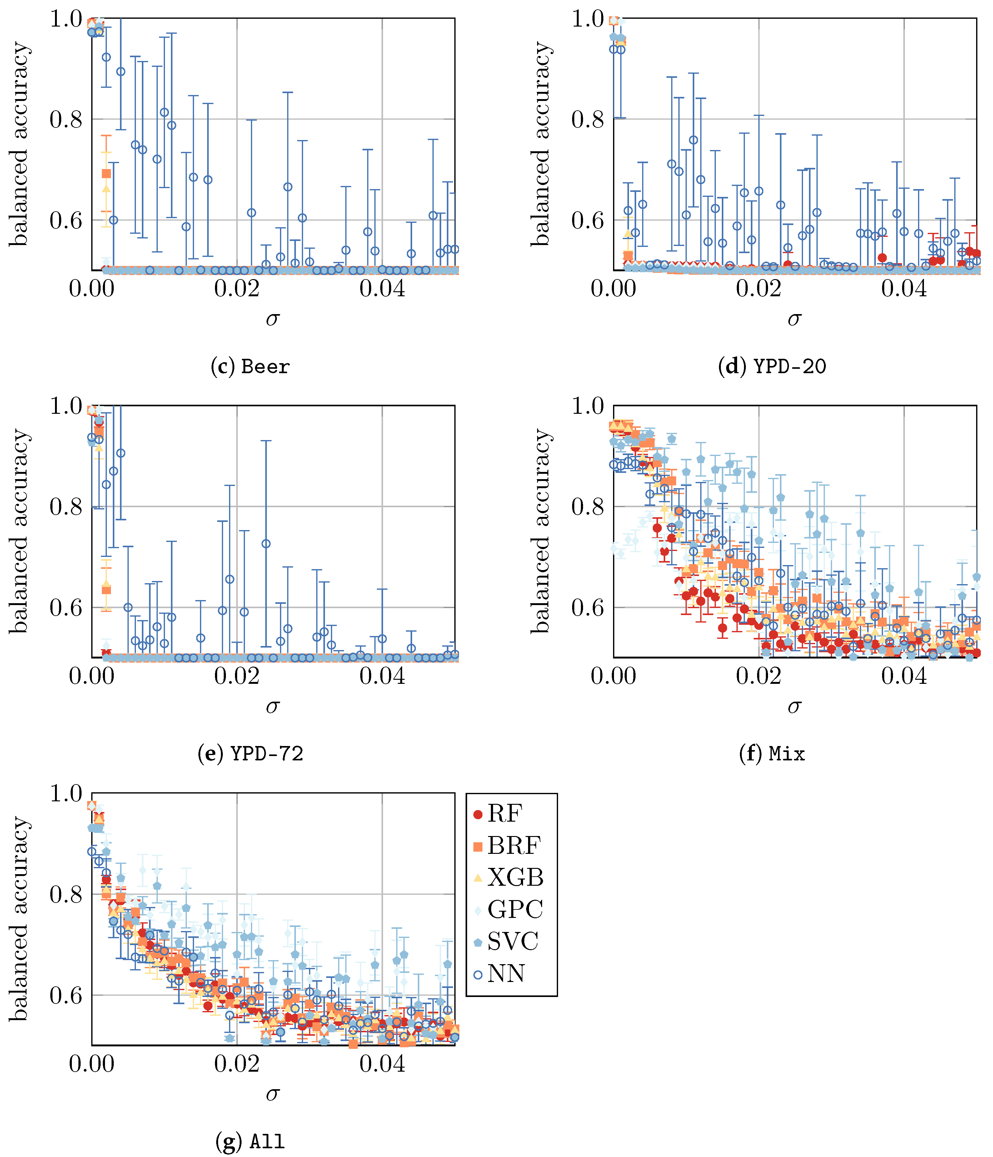
4.4. Yeast Viability under Artificial Noise
In a final study, we compare the model performance using all datasets with artificially imposed noise, as defined in
Section 3. To summarize, we presume that, in our simple approach, the noise represents the imperfections of an ex vitro measurement. The absolute noise level is controlled by a parameter
, i.e., the larger the
, the noisier the ex vitro environment in which the measurements take place, as visualized in
Appendix B. The results are shown in
Figure 6.
4.5. Comparison of Machine Learning Models
In the previous sections, we trained and tested our ML models of interest on various datasets and have found that the resulting balanced accuracies are mostly in similar ranges. To obtain a better understanding of the competitive performance of the models, we performed a pairwise statistical comparison [
33]. For this purpose, we performed Welch’s
t-test [
34] of the score of every model versus every other for each test and training dataset combination (without artificially imposed noise, i.e.,
). That is, for each test and training dataset combination, we evaluated
statistical tests using the respective 10 balanced accuracies that have been obtained from the 10-fold cross-validation for every model. We considered a model superior to another in a statistically significant way if its mean balanced accuracy is larger and the
p-value from the corresponding test is smaller than 0.05. For larger
p-values, no statistically significant superiority relation can be established. Our test can be considered as an indicator of superiority but might not be statistically conclusive because of the limited amount of data considered in this experiment.
Since we are only interested in models that perform reasonably well, we limit the comparison to models with a mean balanced accuracy of at least
. This rule excludes all models from
Table 5 (a) and
Table 6. The result is presented in
Table 8, where we list the superior models (and their respective inferior models) for each test and training dataset combination from
Table 4,
Table 5 (b), and
Table 7. To summarize, we find that GPC is a superior model for every listed test and training dataset combination. Hence, we consider it as the best overall model for our use case. On the other hand, NN was inferior in all cases and can, therefore, be considered as a less-suited model.
5. Discussion
In this study, we combined RS with predictive ML models to evaluate the prospective real-time monitoring of yeast viability in a biotechnological setting. To this end, six ML approaches (RF, GB, XGB, GPC, SVM, and NN—for a detailed description, see
Section 3.2) were trained and tested on various datasets obtained from in vitro RS measurements with the goal of evaluating their performances. The measurements were performed on yeast in different background media and a mixed setting. As summarized in the following, our study is divided into four parts.
In the first part of the study, we considered a viability prediction for yeast in water (control). The resulting mean balanced accuracies (higher is better) are similar for five ML approaches, ranging from 0.81 for XGB to 0.84 for SVM, where only NN performed significantly worse with 0.76. Despite the small dataset of only 722 spectra to analyze, the reasonably good predictive performances of most approaches validate our proof-of-concept for the prediction of yeast viability in an in vitro scenario.
In the second part of the study, we considered yeast that was prepared in background media other than water. Our results revealed that ML models trained on water samples showed comparatively low performance when applied to datasets obtained from yeast in different media. With balanced accuracy values around 0.5, which corresponds to a random guess, the transfer of models trained on water to other media and mixtures is considered not applicable. However, the direct training of ML models on the respective datasets of yeast in media revealed a highly improved balanced accuracy that is comparable to a water medium. Furthermore, combining all datasets for ML training did not yield good, balanced accuracy scores as separate training and prediction for each medium. These findings clearly show the great influence of the background media used for yeast cultivation, reflecting more realistic conditions in biotechnological processes.
In the third part of the study, we considered the contamination with an undesired strain, such as D. bruxellensis yeast that occurs during wine production. For this purpose, samples were spiked with this artificial contaminant. The analysis yielded poor results for the predictive capabilities of ML models on such data, showing a balanced accuracy that is only slightly above 0.5. However, we cannot rule out that the poor performance is due to the experimental setup, as the spiked samples were made in the H2O background.
Finally, in the fourth part of the study, we considered artificially imposed noise on the data. As expected, such noise led to a decrease in model performance for all datasets. For the
Beer,
Apple,
YPD-20, and
YPD-72 datasets, the performance drops (almost) immediately, whereas for the
H2O,
Mix, and
All datasets, a slower decline was observed. For
Apple,
Beer,
YPD-20, and
YPD-72, NN is the most resilient ML approach that can—in some very noisy cases—lead to a model with reasonably good performance. Similarly, for
Mix and
All, the three approaches—GPC, SVM, and NN—are the most resilient ones. Finally, the most resilient approaches for
H2O are GPC and SVM. In summary, a small amount of noise (
) can be mitigated by the models, but with larger noise (
), the predictions become highly unreliable. Since the evaluation of more “realistic samples” (e.g., acquired from the production process of a brewery) were not the subject of this work, we could not verify if the artificially generated noise used in this study corresponds to a real process setting. Consequently, we have no information about the magnitude of
either. However, such knowledge is considered mandatory to assess the practical implications of our findings and will be evaluated in future experiments. This will further facilitate the understanding of uncertainties and their impacts on collected datasets. However, the relative robustness of certain ML models to a small amount of artificial noise indicates that it is possible to transfer classifiers trained in a less noisy environment to a somewhat more noisy environment. Monitoring models using RS combined with various other ML models has already proven to be reasonable for the accurate monitoring of the yeast fermentation process [
35].
A conclusive comparison of the considered ML approaches for different datasets revealed that GPC is the best overall ML approach, whereas NN is the worst. The relatively poor performance of NN may be the result of the chosen network architecture for the NAS. With a different architecture, the results could, in principle, differ significantly. However, in regard to artificial noise, we found that the NN can lead to very noise-resilient models in a noise regime where other approaches fail.
6. Conclusions
In this study, we evaluated the potential of RS and predictive ML models for the discrimination of viable and heat-inactivated S. cerevisiae cells in different background media and a mixed setting. To this end, limited amounts of in vitro measurement data were used to train a total of six different types of models: RF, GB, GPC, SVM, XGB, and NN. We demonstrate that the viability of yeast in a water medium can be predicted with a balanced accuracy of up to 0.84 using SVM with suitable preprocessing of RS data. Similar results could also be achieved for other media. It was only for the mixed setting—where other yeast strains were also present in the sample—that the best-balanced accuracy reached 0.56 using GPC. From statistical tests, GPC has proven to be the best overall ML approach in a direct comparison with the other approaches.
We also discovered that a model trained exclusively with data from yeast in water performs poorly when predicting yeast in other media than water. Thus, we demonstrated that the background medium has a significant influence on the composition of the spectra. Moreover, these observations clearly show that the robustness of model predictions is closely related to the sample composition used for training. We expect a more accurate and robust prediction when the training of ML models is performed on larger datasets from an experimental environment reflecting “real world” conditions.
In summary, our results demonstrate that RS, in combination with ML, is a promising tool for non-invasive inline monitoring of fermentation processes. We were able to demonstrate a working proof-of-concept for our in vitro scenario. Optionally, RS can be used in combination with already established analytical methods, such as for CO, turbidity, or temperature. Furthermore, RS allows measuring sugar consumption and ethanol production, providing an even more detailed analytic view of ongoing fermentation processes. On the other hand, the prediction performances of the presented ML models still need to be improved, which could be achieved with a larger set of Raman spectra or special-purpose models that have been optimized for this particular task. The realization of such models could serve as a possible starting point for further research.
Author Contributions
Conceptualization, S.M.B. and M.B.; methodology, J.W., R.H., S.M.B. and M.B.; software, R.H. and M.B.; validation, J.W. and R.H.; formal analysis, R.H. and M.B; investigation, J.W. and R.H.; resources, J.W., S.M.B., R.H. and M.B.; data curation, R.H.; writing—original draft preparation, C.R., J.W., R.H., S.M.B. and M.B.; writing—review and editing, C.R., J.W., R.H., S.M.B. and M.B.; visualization, R.H.; supervision, S.M.B. and M.B.; project administration, R.H.; funding acquisition, M.B. All authors have read and agreed to the published version of the manuscript.
Funding
This research was funded in parts by DFG (Deutsche Forschungsgemeinschaft) within the priority program SPP 2331 under grant number BO 2538/5-1.
Data Availability Statement
The data presented in this study are available upon request.
Acknowledgments
R.H. and M.B. gratefully acknowledge funding from DFG within the priority program SPP 2331 under grant number BO 2538/5-1. The authors acknowledge Lukas Kriem for support with the Raman measurements.
Conflicts of Interest
The authors declare no conflict of interest.
Abbreviations
The following abbreviations are used in this manuscript:
| D. bruxellensis | Dekkera bruxellensis |
| XGB | EXtreme Gradient Boosting classifier |
| GPC | Gaussian process classifier |
| GB | Gradient boosting classifier |
| ML | Machine learning |
| NAS | Neural architecture search |
| NN | Neural network |
| PAT | Process analytical technology |
| RS | Raman spectroscopy |
| RF | Random forest classifier |
| S. cerevisiae | Saccharomyces cerevisiae |
| SVM | Support vector machine classifier |
| YPD | Yeast extract peptone dextrose |
Appendix A. Formal Data-Processing Pipeline
In this appendix section, we formally describe our data-processing pipeline from
Section 3. As indicated in
Section 3, we omit all measurement units to simplify the notation.
Appendix A.1. Data Processing
We preprocessed the data into a unified form that is suitable for ML applications. For each data point n, five preprocessing steps were used:
Summarized, the effective preprocessing transformation
leads to the data shown in
Appendix B.
Appendix A.2. Artificial Noise
We also considered data that have been perturbed by artificially generated noise. For this purpose, we extended the preprocessing transformation, (
A12), by an additional step after the first rescaling, (
A3), i.e., between steps two and three. In this additional step, we performed a perturbation
by applying
where
denotes random variables drawn from a normal distribution with the vanishing mean and standard deviation
. For the noiseless case
, we set the constant value
. To summarize, the perturbed preprocessing transformation is given by
instead of (
A12).
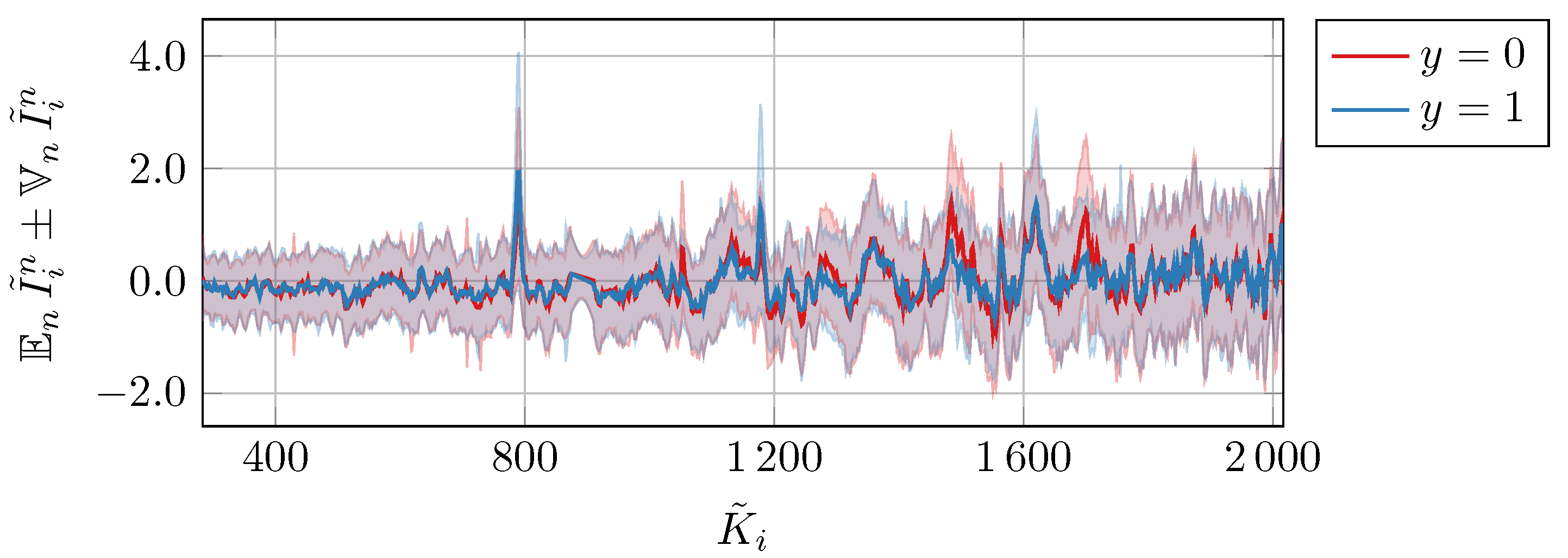
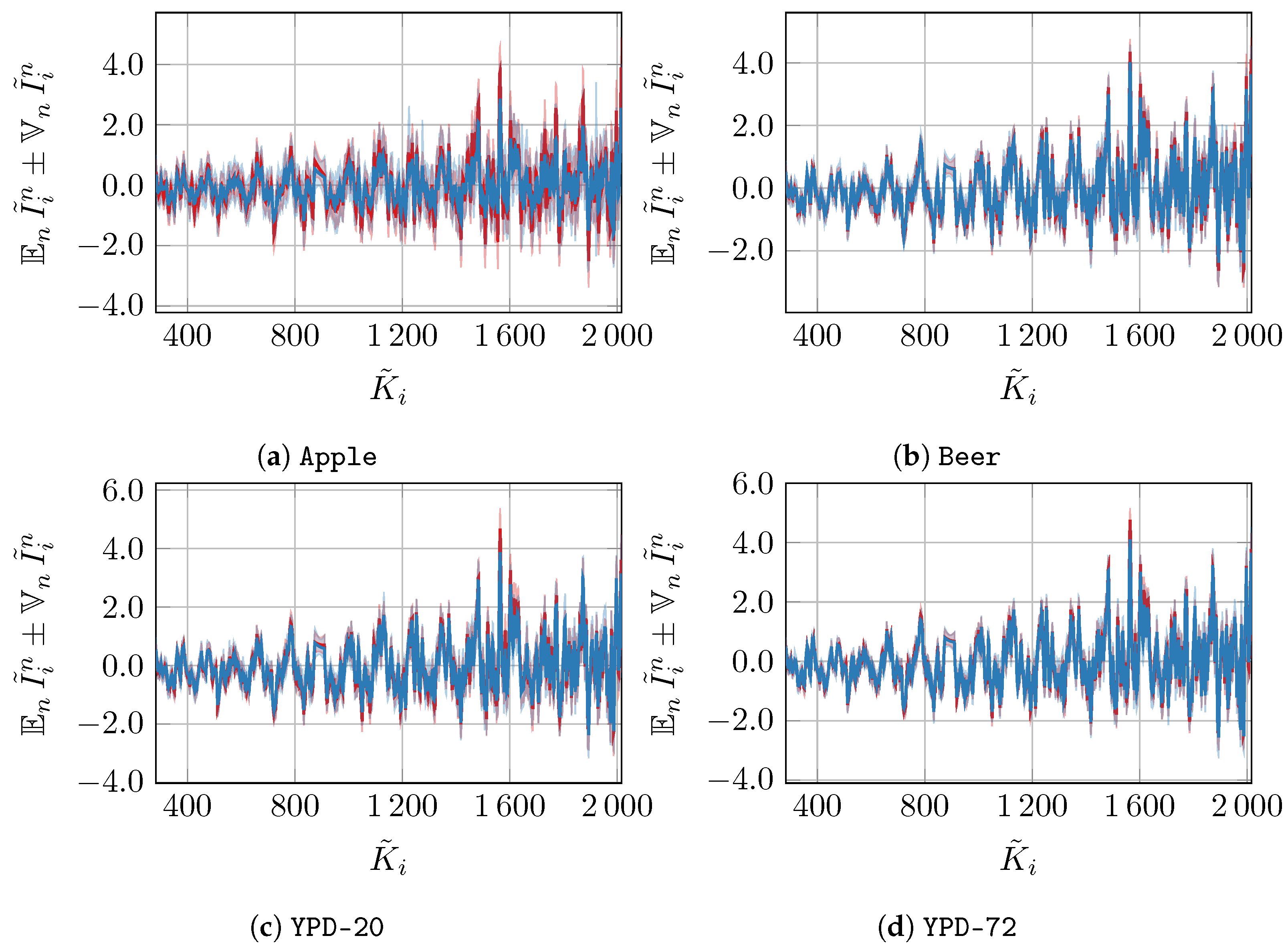
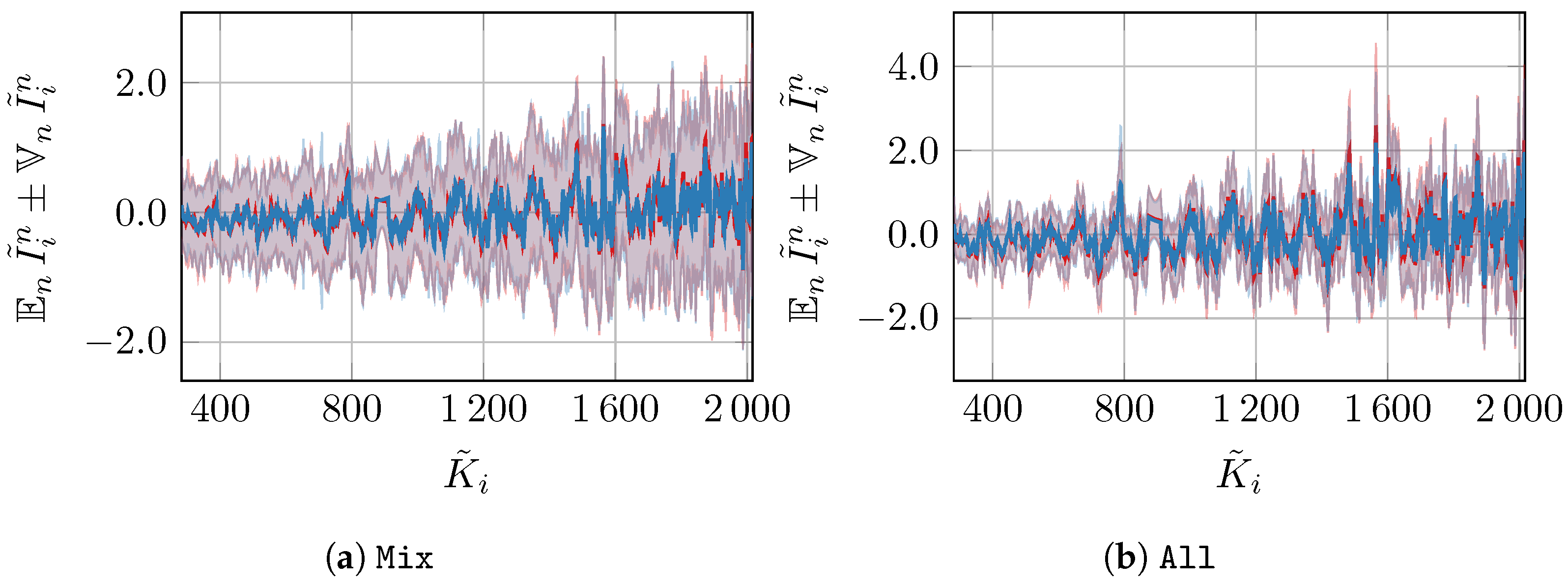
Appendix B. Data Visualization
In this appendix section, we visualize the datasets that resulted from our preprocessing method, which is explained in
Appendix A. In
Figure A1,
Figure A2 and
Figure A3, we show the mean
and standard deviation
of each preprocessed dataset, divided into data for
(yeast viable) and
(yeast heat-inactivated). As indicated in
Section 3, we omit all measurement units. To demonstrate the effects of different values of
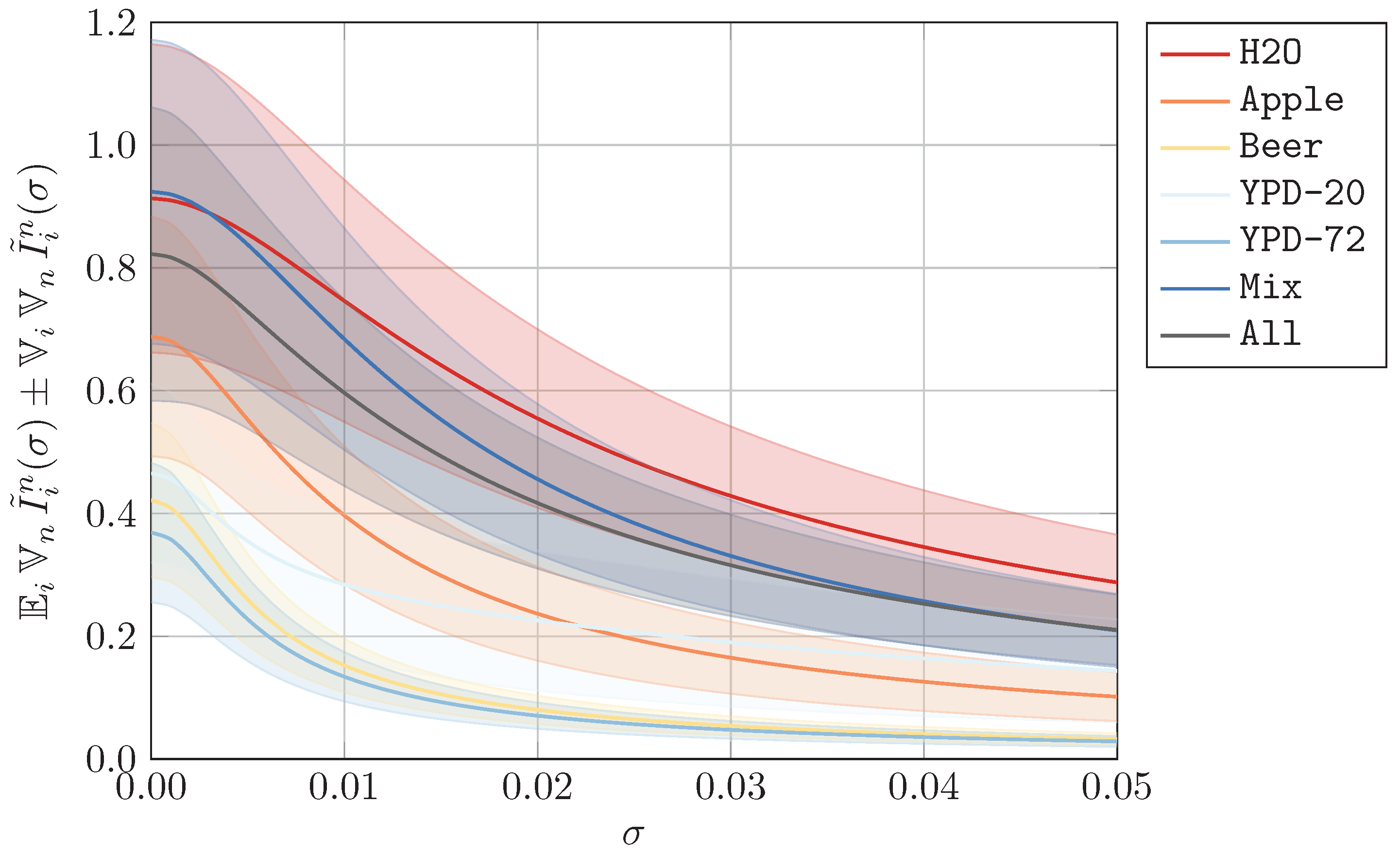
from artificial noise, we additionally plot the expected standard deviation over all wavelengths
in
Figure A4, where we also show the corresponding standard deviation
. As expected, the signal-to-noise ratio decreases as the perturbation increases.
Figure A1.
Mean and standard deviation of all datasets from
Table 1 after the preprocessing.
Figure A1.
Mean and standard deviation of all datasets from
Table 1 after the preprocessing.
Figure A2.
Mean and standard deviation of all datasets from
Table 2 in analogy to
Figure A1.
Figure A2.
Mean and standard deviation of all datasets from
Table 2 in analogy to
Figure A1.
Figure A3.
Mean and standard deviation of all datasets from
Table 3 in analogy to
Figure A1.
Figure A3.
Mean and standard deviation of all datasets from
Table 3 in analogy to
Figure A1.
Figure A4.
Mean and standard deviation for artificially perturbed data as defined in
Section 3.
Figure A4.
Mean and standard deviation for artificially perturbed data as defined in
Section 3.
Appendix C. Machine Learning Model Specifications
In this appendix section, we list the details of the chosen ML approaches from
Section 3:
RF: We used the implementation
RandomForestClassifier from scikit-learn [
32] with the parameter
.
GB: We used the implementation
HistGradientBoostingClassifier from scikit-learn [
32] with the parameter
.
XGB: We used the implementation
XGBClassifier from [
37].
GPC: We used the implementation
GaussianProcessClassifier from scikit-learn [
32] with the parameters
and
.
SVM: We used the implementation
SVC from scikit-learn [
32] with the parameter
.
NN: We used PyTorch [
38] with Keras [
39] and Optuna [
40] to realize the neural network. To this end, we utilized NAS to determine the structure of the network. In total, we specified nine NAS parameters that are all defined within the Optuna framework:
- (a)
,
- (b)
,
- (c)
,
- (d)
,
- (e)
,
- (f)
,
- (g)
,
- (h)
and
- (i)
.
Based on these parameters, the neural network was created as follows:
- (a)
An input layer keras.layers.Input is followed by
- (b)
layers with the following options:
, , and , according to the respective NAS parameter,
,
,
, and
.
Each layer is followed by .
- (c)
If is non-zero, the convolutional layers are finalized with , otherwise, is used.
- (d)
Next, layers are added with the following options:
according to the respective NAS parameter,
,
, and
.
- (e)
If is one, each dense layer is supplemented by .
- (f)
Finally, the output layer is added with the following options:
,
,
, and
.
The neural networks were trained with with the following options:
- (a)
according to the respective NAS parameter and
- (b)
A validation split of on the sparse categorical cross-entropy loss function.
In addition, we made use of the callback functions and , respectively, during the training procedure. The neural network test accuracy score averaged over all stratified 10-folds was chosen as the NAS goal function.
For all unspecified parameters, the default values of the respective implementations were used.
References
- Spencer, J.F.; Spencer, D.M. Yeasts in Natural and Artificial Habitats; Springer Science & Business Media: Berlin/Heidelberg, Germany, 1997. [Google Scholar]
- Gibson, B.R.; Lawrence, S.J.; Leclaire, J.P.; Powell, C.D.; Smart, K.A. Yeast responses to stresses associated with industrial brewery handling. FEMS Microbiol. Rev. 2007, 31, 535–569. [Google Scholar] [CrossRef] [PubMed]
- Matallana, E.; Aranda, A. Biotechnological impact of stress response on wine yeast. Lett. Appl. Microbiol. 2017, 64, 103–110. [Google Scholar] [CrossRef] [PubMed]
- Baradez, M.O.; Biziato, D.; Hassan, E.; Marshall, D. Application of Raman Spectroscopy and Univariate Modelling As a Process Analytical Technology for Cell Therapy Bioprocessing. Front. Med. 2018, 5, 47. [Google Scholar] [CrossRef]
- Boyd, A.R.; Gunasekera, T.S.; Attfield, P.V.; Simic, K.; Vincent, S.F.; Veal, D.A. A flow-cytometric method for determination of yeast viability and cell number in a brewery. FEMS Yeast Res. 2003, 3, 11–16. [Google Scholar] [CrossRef] [PubMed]
- Pierce, J.; Committee, A. Institute of Brewing: Analysis committee measurement of yeast viability. J. Inst. Brew. 1970, 76, 442–443. [Google Scholar] [CrossRef]
- Boulton, C.; Quain, D. Brewing Yeast and Fermentation; Wiley: Hoboken, NJ, USA, 2008. [Google Scholar]
- Thomson, K.; Bhat, A.; Carvell, J. Comparison of a new digital imaging technique for yeast cell counting and viability assessments with traditional methods. J. Inst. Brew. 2015, 121, 231–237. [Google Scholar] [CrossRef]
- Luoma, P.; Golabgir, A.; Brandstetter, M.; Kasberger, J.; Herwig, C. Workflow for multi-analyte bioprocess monitoring demonstrated on inline NIR spectroscopy of P. chrysogenum fermentation. Anal. Bioanal. Chem. 2016, 409, 797–805. [Google Scholar] [CrossRef]
- Hirsch, E.; Pataki, H.; Domján, J.; Farkas, A.; Vass, P.; Fehér, C.; Barta, Z.; Nagy, Z.K.; Marosi, G.J.; Csontos, I. Inline noninvasive Raman monitoring and feedback control of glucose concentration during ethanol fermentation. Biotechnol. Prog. 2019, 35, e2848. [Google Scholar] [CrossRef]
- Wieland, K.; Masri, M.; von Poschinger, J.; Brück, T.; Haisch, C. Non-invasive Raman spectroscopy for time-resolved in-line lipidomics. RSC Adv. 2021, 11, 28565–28572. [Google Scholar] [CrossRef]
- Esmonde-White, K.A.; Cuellar, M.; Lewis, I.R. The role of Raman spectroscopy in biopharmaceuticals from development to manufacturing. Anal. Bioanal. Chem. 2022, 414, 969–991. [Google Scholar] [CrossRef]
- Rösch, P.; Harz, M.; Schmitt, M.; Peschke, K.D.; Ronneberger, O.; Burkhardt, H.; Motzkus, H.W.; Lankers, M.; Hofer, S.; Thiele, H.; et al. Chemotaxonomic identification of single bacteria by micro-Raman spectroscopy: Application to clean-room-relevant biological contaminations. Appl. Environ. Microbiol. 2005, 71, 1626–1637. [Google Scholar] [CrossRef] [PubMed]
- Wulf, M.W.H.; Willemse-Erix, D.; Verduin, C.M.; Puppels, G.; van Belkum, A.; Maquelin, K. The use of Raman spectroscopy in the epidemiology of methicillin-resistant Staphylococcus aureus of human- and animal-related clonal lineages. Clin. Microbiol. Infect. 2011, 18, 147–152. [Google Scholar] [CrossRef]
- Meisel, S.; Stöckel, S.; Elschner, M.; Melzer, F.; Rösch, P.; Popp, J. Raman spectroscopy as a potential tool for detection of Brucella spp. in milk. Appl. Environ. Microbiol. 2012, 78, 5575–5583. [Google Scholar] [CrossRef] [PubMed]
- Stöckel, S.; Meisel, S.; Elschner, M.; Rosch, P.; Popp, J. Identification of Bacillus anthracis via Raman spectroscopy and chemometric approaches. Anal. Chem. 2012, 84, 9873–9880. [Google Scholar] [CrossRef] [PubMed]
- Hamasha, K.; Mohaidat, Q.I.; Putnam, R.A.; Woodman, R.C.; Palchaudhuri, S.; Rehse, S.J. Sensitive and specific discrimination of pathogenic and nonpathogenic Escherichia coli using Raman spectroscopy—A comparison of two multivariate analysis techniques. Biomed. Opt. Express 2013, 4, 481–489. [Google Scholar] [CrossRef]
- Zhu, X.; Xu, T.; Lin, Q.; Duan, Y. Technical Development of Raman Spectroscopy: From Instrumental to Advanced Combined Technologies. Appl. Spectrosc. Rev. 2014, 49, 64–82. [Google Scholar] [CrossRef]
- Yaseen, T.; Sun, D.W.; Cheng, J.H. Raman imaging for food quality and safety evaluation: Fundamentals and applications. Trends Food Sci. Technol. 2017, 62, 177–189. [Google Scholar] [CrossRef]
- Lintvedt, T.A.; Andersen, P.V.; Afseth, N.K.; Marquardt, B.; Gidskehaug, L.; Wold, J.P. Feasibility of In-Line Raman Spectroscopy for Quality Assessment in Food Industry: How Fast Can We Go? Appl. Spectrosc. 2022, 76, 559–568. [Google Scholar] [CrossRef]
- Khan, H.H.; McCarthy, U.; Esmonde-White, K.; Casey, I.; O’Shea, N. Potential of Raman spectroscopy for in-line measurement of raw milk composition. Food Control 2023, 152, 109862. [Google Scholar] [CrossRef]
- Woolfit, M.; Rozpedowska, E.; Piskur, J.; Wolfe, K.H. Genome survey sequencing of the wine spoilage yeast Dekkera (Brettanomyces) bruxellensis. Eukaryot Cell 2007, 6, 721–733. [Google Scholar] [CrossRef]
- Bishop, C.M. Pattern Recognition and Machine Learning; Springer: Berlin/Heidelberg, Germany, 2006. [Google Scholar]
- James, G.; Witten, D.; Hastie, T.; Tibshirani, R.; Taylor, J. An Introduction to Statistical Learning: With Applications in Python; Springer Texts in Statistics; Springer International Publishing: Berlin/Heidelberg, Germany, 2023. [Google Scholar]
- Breiman, L. Random Forests. Mach. Learn. 2001, 45, 5–32. [Google Scholar] [CrossRef]
- Friedman, J.H. Greedy function approximation: A gradient boosting machine. Ann. Stat. 2001, 29, 1189–1232. [Google Scholar] [CrossRef]
- Chen, T.; Guestrin, C. XGBoost. In Proceedings of the 22nd ACM SIGKDD International Conference on Knowledge Discovery and Data Mining, San Francisco, CA, USA, 13–17 August 2016. [Google Scholar] [CrossRef]
- Rasmussen, C.E.; Williams, C.K.I. Gaussian Processes for Machine Learning; MIT Press: Cambridge, MA, USA, 2005. [Google Scholar]
- Cortes, C.; Vapnik, V. Support-vector networks. Mach. Learn. 1995, 20, 273–297. [Google Scholar] [CrossRef]
- Cervantes, J.; Garcia-Lamont, F.; Rodríguez-Mazahua, L.; Lopez, A. A comprehensive survey on support vector machine classification: Applications, challenges and trends. Neurocomputing 2020, 408, 189–215. [Google Scholar] [CrossRef]
- Schmidhuber, J. Deep learning in neural networks: An overview. Neural Netw. 2015, 61, 85–117. [Google Scholar] [CrossRef]
- Pedregosa, F.; Varoquaux, G.; Gramfort, A.; Michel, V.; Thirion, B.; Grisel, O.; Blondel, M.; Prettenhofer, P.; Weiss, R.; Dubourg, V.; et al. Scikit-learn: Machine Learning in Python. J. Mach. Learn. Res. 2011, 12, 2825–2830. [Google Scholar]
- Dietterich, T.G. Approximate Statistical Tests for Comparing Supervised Classification Learning Algorithms. Neural Comput. 1998, 10, 1895–1923. [Google Scholar] [CrossRef] [PubMed]
- Welch, B.L. The generalization of Student’s Problem when several different population variances are involved. Biometrika 1947, 34, 28–35. [Google Scholar] [CrossRef]
- Jiang, H.; Xu, W.; Ding, Y.; Chen, Q. Quantitative analysis of yeast fermentation process using Raman spectroscopy: Comparison of CARS and VCPA for variable selection. Spectrochim. Acta Part A Mol. Biomol. Spectrosc. 2020, 228, 117781. [Google Scholar] [CrossRef]
- Baek, S.J.; Park, A.; Ahn, Y.J.; Choo, J. Baseline correction using asymmetrically reweighted penalized least squares smoothing. Analyst 2015, 140, 250–257. [Google Scholar] [CrossRef]
- dmlc GitHub. XGBoost Python Package. 2022. Available online: https://github.com/dmlc/xgboost/tree/master/python-package (accessed on 6 December 2022).
- Paszke, A.; Gross, S.; Massa, F.; Lerer, A.; Bradbury, J.; Chanan, G.; Killeen, T.; Lin, Z.; Gimelshein, N.; Antiga, L.; et al. PyTorch: An Imperative Style, High-Performance Deep Learning Library. In Advances in Neural Information Processing Systems 32; Wallach, H., Larochelle, H., Beygelzimer, A., d’ Alché-Buc, F., Fox, E., Garnett, R., Eds.; Curran Associates, Inc.: Red Hook, NY, USA, 2019; pp. 8024–8035. [Google Scholar]
- Chollet, F. Keras. 2015. Available online: https://keras.io (accessed on 6 December 2022).
- Akiba, T.; Sano, S.; Yanase, T.; Ohta, T.; Koyama, M. Optuna: A Next-generation Hyperparameter Optimization Framework. In Proceedings of the 25rd ACM SIGKDD International Conference on Knowledge Discovery and Data Mining, Anchorage, AK, USA, 4–8 August 2019. [Google Scholar]
| Disclaimer/Publisher’s Note: The statements, opinions and data contained in all publications are solely those of the individual author(s) and contributor(s) and not of MDPI and/or the editor(s). MDPI and/or the editor(s) disclaim responsibility for any injury to people or property resulting from any ideas, methods, instructions or products referred to in the content. |
© 2023 by the authors. Licensee MDPI, Basel, Switzerland. This article is an open access article distributed under the terms and conditions of the Creative Commons Attribution (CC BY) license (https://creativecommons.org/licenses/by/4.0/).


