
Characterization of the Aeration and Hydrodynamics in Vertical-Wheel™ Bioreactors

 , , ,
, , ,  , , , ,
  , and
, and
Abstract
: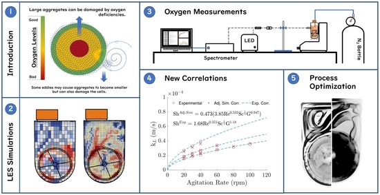
1. Introduction
2. Materials and Methods
2.1. About the PBS MINI™
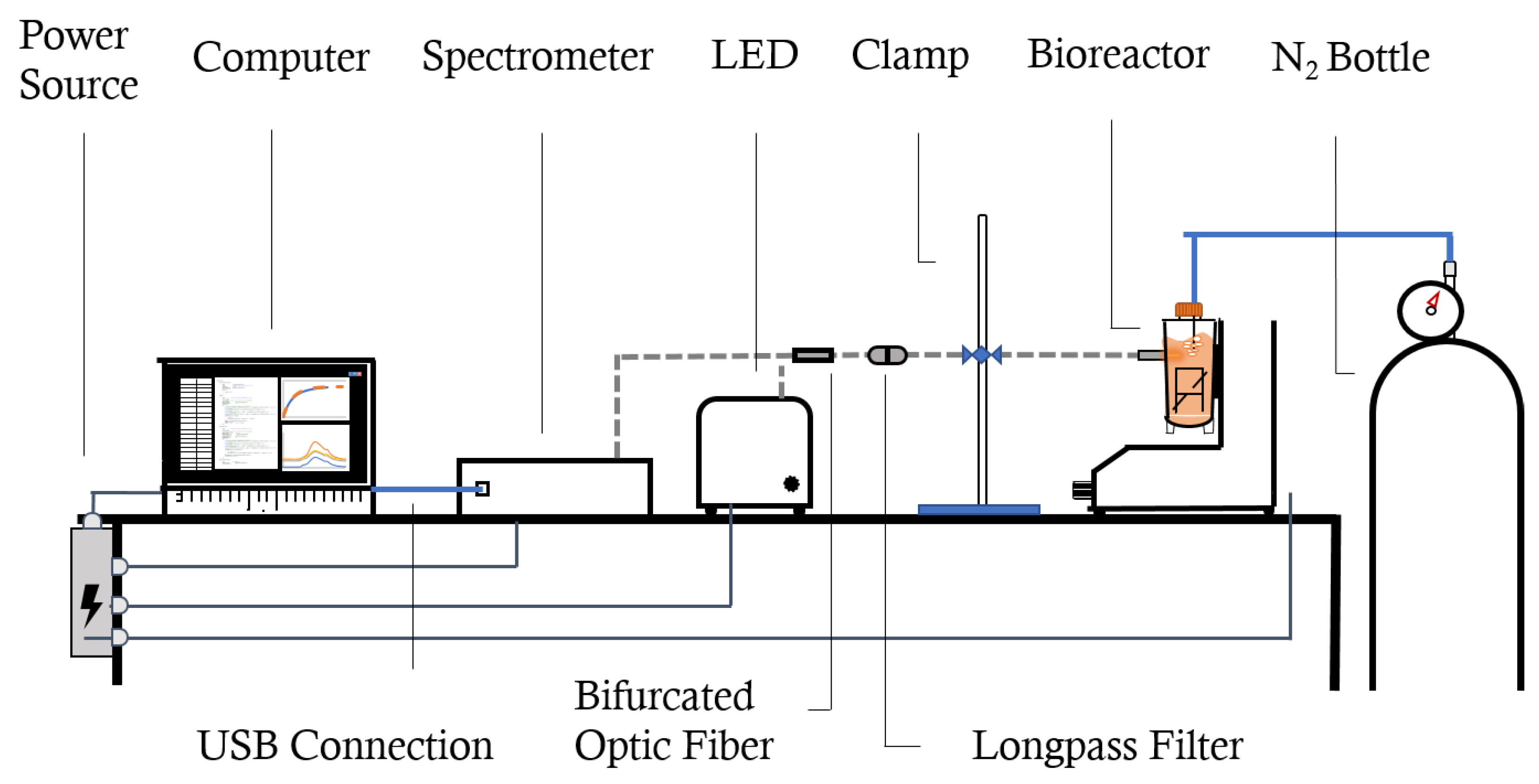
2.2. Experimental Protocol: Spectroscopy-Based Oxygen Measurements
2.3. Data Treatment
2.4. Transport Equations and Turbulence Model
2.5. Sub-Grid Scale Model
2.6. Mass Transfer Model
2.7. In Silico Protocol
2.8. Post-Processing: Mass Transfer
2.9. Post-Processing: Turbulent Variables
2.10. Post-Processing: Mesh Refinement Quality
2.11. Maximum Cell Density
3. Results
3.1. Oxygen Mass Transfer: Experimental Evaluation and Numerical Predictions
3.2. Simulation Results
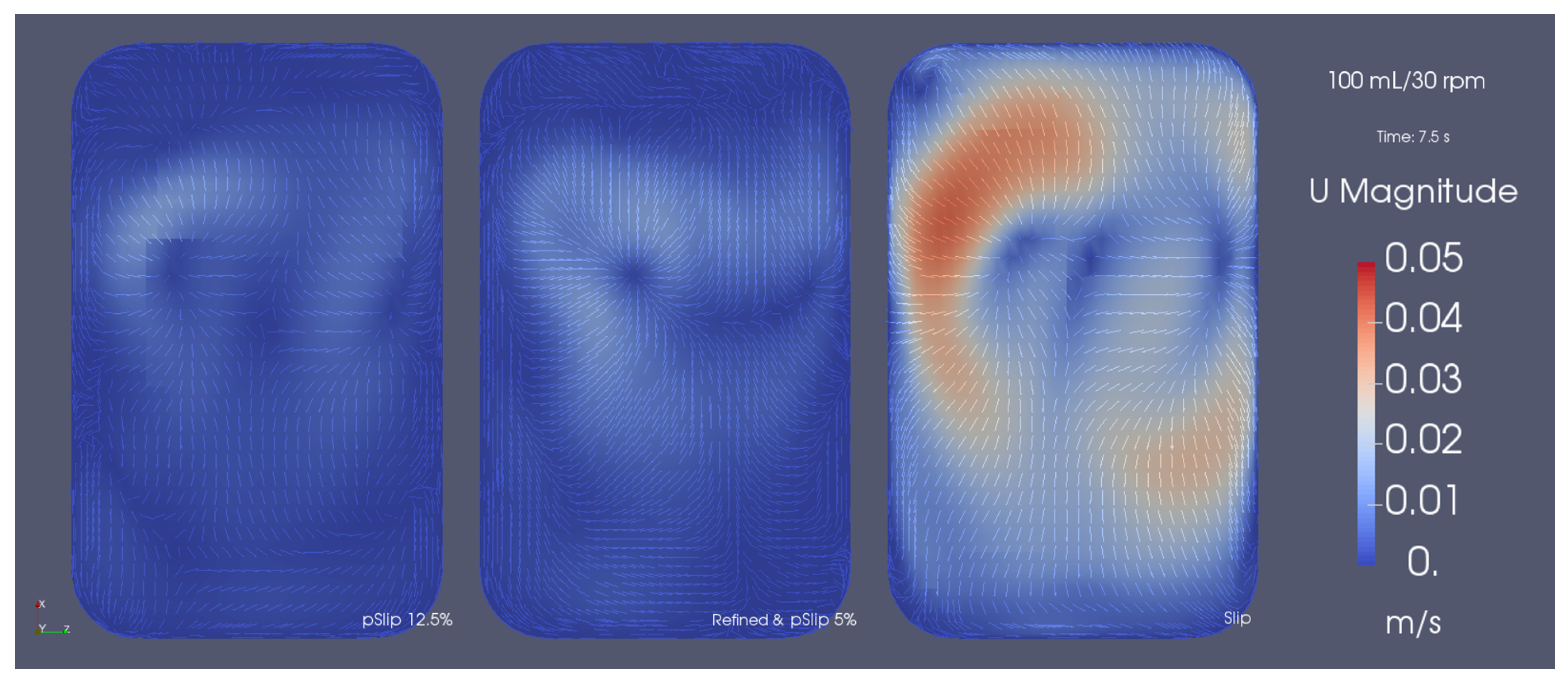
3.3. Mesh Refinement Study
3.4. Mass Transfer Mechanisms
3.5. Characterization of the Flow
3.6. Hydrodynamic Analysis
4. Discussion
4.1. Experimental Work
4.2. Simulation and Numerical Predictions of the Aeration
4.3. Flow and Hydrodynamics
5. Conclusions
Supplementary Materials
Author Contributions
Funding
Institutional Review Board Statement
Informed Consent Statement
Data Availability Statement
Conflicts of Interest
Abbreviations
| AMI | Arbitrary Mesh Interface |
| BC | Boundary Condition |
| CBL | Concentration Boundary Layer |
| CFD | Computational Fluid Dynamics |
| CFL | Courant–Friedrichs–Lewy |
| EDR | Energy Dissipation Rate |
| MDPI | Multidisciplinary Digital Publishing Institute |
| LES | Large Eddy Simulation |
| SGS | Sub-Grid Scale |
| LSM | Least Squares Method |
| OTR | Oxygen Transfer Rate |
| OUR | Oxygen Uptake Rate |
| RANS | Reynolds Averaged Navier Stokes |
| UV-Vis-NIR | Ultraviolet, Visible and Near-Infrared |
| WALE | Wall Adapting Local Eddy Viscosity |
References
- Kim, H.J.; Park, J.S. Usage of human mesenchymal stem cells in cell-based therapy: Advantages and disadvantages. Dev. Reprod. 2017, 21, 1. [Google Scholar] [CrossRef] [PubMed]
- Borys, B.S.; Dang, T.; So, T.; Rohani, L.; Revay, T.; Walsh, T.; Thompson, M.; Argiropoulos, B.; Rancourt, D.E.; Jung, S.; et al. Overcoming bioprocess bottlenecks in the large-scale expansion of high-quality hiPSC aggregates in vertical-wheel stirred suspension bioreactors. Stem Cell Res. Ther. 2021, 12, 1–19. [Google Scholar] [CrossRef] [PubMed]
- Rodrigues, C.A.; Silva, T.P.; Nogueira, D.E.; Fernandes, T.G.; Hashimura, Y.; Wesselschmidt, R.; Diogo, M.M.; Lee, B.; Cabral, J.M. Scalable culture of human induced pluripotent cells on microcarriers under xeno-free conditions using single-use vertical-wheel™ bioreactors. J. Chem. Technol. Biotechnol. 2018, 93, 3597–3606. [Google Scholar] [CrossRef]
- Nogueira, D.E.; Rodrigues, C.A.; Carvalho, M.S.; Miranda, C.C.; Hashimura, Y.; Jung, S.; Lee, B.; Cabral, J. Strategies for the expansion of human induced pluripotent stem cells as aggregates in single-use Vertical-Wheel™ bioreactors. J. Biol. Eng. 2019, 13, 1–14. [Google Scholar] [CrossRef] [PubMed]
- de Sousa Pinto, D.; Bandeiras, C.; de Almeida Fuzeta, M.; Rodrigues, C.A.; Jung, S.; Hashimura, Y.; Tseng, R.J.; Milligan, W.; Lee, B.; Ferreira, F.C.; et al. Scalable manufacturing of human mesenchymal stromal cells in the vertical-wheel bioreactor system: An experimental and economic approach. Biotechnol. J. 2019, 14, 1800716. [Google Scholar] [CrossRef] [PubMed]
- de Almeida Fuzeta, M.; Bernardes, N.; Oliveira, F.D.; Costa, A.C.; Fernandes-Platzgummer, A.; Farinha, J.P.; Rodrigues, C.A.; Jung, S.; Tseng, R.J.; Milligan, W.; et al. Scalable production of human mesenchymal stromal cell-derived extracellular vesicles under serum-/xeno-free conditions in a microcarrier-based bioreactor culture system. Front. Cell Dev. Biol. 2020, 8, 553444. [Google Scholar] [CrossRef] [PubMed]
- Gareau, T.; Lara, G.G.; Shepherd, R.D.; Krawetz, R.; Rancourt, D.E.; Rinker, K.D.; Kallos, M.S. Shear stress influences the pluripotency of murine embryonic stem cells in stirred suspension bioreactors. J. Tissue Eng. Regen. Med. 2014, 8, 268–278. [Google Scholar] [CrossRef] [PubMed]
- Stolberg, S.; McCloskey, K.E. Can shear stress direct stem cell fate? Biotechnol. Prog. 2009, 25, 10–19. [Google Scholar] [CrossRef] [PubMed]
- Cherry, R.; Papoutsakis, E. Hydrodynamic effects on cells in agitated tissue culture reactors. Bioprocess Eng. 1986, 1, 29–41. [Google Scholar] [CrossRef]
- Van Winkle, A.P.; Gates, I.D.; Kallos, M.S. Mass transfer limitations in embryoid bodies during human embryonic stem cell differentiation. Cells Tissues Organs 2012, 196, 34–47. [Google Scholar]
- Wu, J.; Rostami, M.R.; Cadavid Olaya, D.P.; Tzanakakis, E.S. Oxygen transport and stem cell aggregation in stirred-suspension bioreactor cultures. PLoS ONE 2014, 9, e102486. [Google Scholar] [CrossRef] [PubMed]
- Borys, B.S.; Le, A.; Roberts, E.L.; Dang, T.; Rohani, L.; Hsu, C.Y.M.; Wyma, A.A.; Rancourt, D.E.; Gates, I.D.; Kallos, M.S. Using computational fluid dynamics (CFD) modeling to understand murine embryonic stem cell aggregate size and pluripotency distributions in stirred suspension bioreactors. J. Biotechnol. 2019, 304, 16–27. [Google Scholar] [CrossRef] [PubMed]
- Muhammad, N. Finite volume method for simulation of flowing fluid via OpenFOAM. Eur. Phys. J. Plus 2021, 136, 1–22. [Google Scholar] [CrossRef]
- Liovic, P.; Šutalo, I.D.; Stewart, R.; Glattauer, V.; Meagher, L. Fluid flow and stresses on microcarriers in spinner flask bioreactors. In Proceedings of the 9th International Conference on CFD in the Minerals and Process Industries, Melbourne, Australia, 10–12 December 2012; CSIRO: Canberra, Australia, 2012. [Google Scholar]
- Berry, J.; Liovic, P.; Šutalo, I.; Stewart, R.; Glattauer, V.; Meagher, L. Characterisation of stresses on microcarriers in a stirred bioreactor. Appl. Math. Model. 2016, 40, 6787–6804. [Google Scholar] [CrossRef]
- Ghasemian, M.; Layton, C.; Nampe, D.; zur Nieden, N.I.; Tsutsui, H.; Princevac, M. Hydrodynamic characterization within a spinner flask and a rotary wall vessel for stem cell culture. Biochem. Eng. J. 2020, 157, 107533. [Google Scholar] [CrossRef]
- Davies, J. The effects of surface films in damping eddies at a free surface of a turbulent liquid. Proc. R. Soc. Ser. Math. Phys. Sci. 1966, 290, 515–526. [Google Scholar]
- Zappa, C.J.; Asher, W.E.; Jessup, A.T. Microscale wave breaking and air-water gas transfer. J. Geophys. Res. 2001, 106, 9385–9391. [Google Scholar] [CrossRef]
- Theofanous, T. Conceptual models of gas exchange. In Gas Transfer at Water Surfaces; Springer: Dordrecht, The Netherlands, 1984; pp. 271–281. [Google Scholar]
- Dang, T.; Borys, B.S.; Kanwar, S.; Colter, J.; Worden, H.; Blatchford, A.; Croughan, M.S.; Hossan, T.; Rancourt, D.E.; Lee, B.; et al. Computational fluid dynamic characterization of vertical-wheel bioreactors used for effective scale-up of human induced pluripotent stem cell aggregate culture. Can. J. Chem. Eng. 2021, 99, 2536–2553. [Google Scholar] [CrossRef]
- PBS Biotech Offcial Website. Available online: https://www.pbsbiotech.com/ (accessed on 1 August 2021).
- PBS Biotech MINI User Manual. Available online: https://www.pbsbiotech.com/uploads/1/7/9/9/17996975/pbs_mini_user_manual_il00266_rev_c.pdf (accessed on 1 August 2021).
- MATLAB. 9.6.0.1072779 (R2019a); The MathWorks Inc.: Natick, MA, USA, 2019. [Google Scholar]
- Sugano, Y.; Ratkowsky, D. Effect of transverse vibration upon the rate of mass transfer from horizontal cylinders. Chem. Eng. Sci. 1968, 23, 707–716. [Google Scholar] [CrossRef]
- Middleman, S. An introduction to mass and heat transfer: Principles of analysis and design. Eur. J. Eng. Educ. 1998, 23, 397. [Google Scholar]
- Bird, R.B. Transport phenomena. Appl. Mech. Rev. 2002, 55, R1–R4. [Google Scholar] [CrossRef]
- Cussler, E.L.; Cussler, E.L. Diffusion: Mass Transfer in Fluid Systems; Cambridge University Press: Cambridge, UK, 2009. [Google Scholar]
- Kestin, J.; Sokolov, M.; Wakeham, W.A. Viscosity of liquid water in the range −8 °C to 150 °C. J. Phys. Chem. Ref. Data 1978, 7, 941–948. [Google Scholar] [CrossRef]
- Engineering ToolBox. Diffusion Coefficients of Gases in Water. 2008. Available online: https://www.engineeringtoolbox.com/diffusion-coefficients-d_1404.html (accessed on 11 October 2021).
- Oxygen Diffususion Coefficients in Water. Available online: http://compost.css.cornell.edu/oxygen/oxygen.diff.water.html (accessed on 11 October 2021).
- Holmén, K.; Liss, P. Models for air-water gas transfer: An experimental investigation. Tellus Chem. Phys. Meteorol. 1984, 36, 92–100. [Google Scholar] [CrossRef]
- Welty, J.; Rorrer, G.L.; Foster, D.G. Fundamentals of Momentum, Heat, and Mass Transfer; John Wiley & Sons: Hoboken, NJ, USA, 2020. [Google Scholar]
- St-Denis, C.; Fell, C. Diffusivity of oxygen in water. Can. J. Chem. Eng. 1971, 49, 885. [Google Scholar] [CrossRef]
- Ramsing, N.; Gundersen, J. Seawater and gases. Limnol. Ocean. 2011, 37, 1307–1312. [Google Scholar]
- Chen, J.; Kim, H.D.; Kim, K.C. Measurement of dissolved oxygen diffusion coefficient in a microchannel using UV-LED induced fluorescence method. Microfluid. Nanofluid. 2013, 14, 541–550. [Google Scholar] [CrossRef]
- Ju, L.K.; Ho, C.S. Oxygen diffusion coefficient and solubility in n-hexadecane. Biotechnol. Bioeng. 1989, 34, 1221–1224. [Google Scholar] [CrossRef]
- Moukalled, F.; Mangani, L.; Darwish, M. The Finite Volume Method in Computational Fluid Dynamics; Springer: Berlin/Heidelberg, Germany, 2016; Volume 113. [Google Scholar]
- Donzis, D.A.; Aditya, K.; Sreenivasan, K.; Yeung, P. The turbulent Schmidt number. J. Fluids Eng. 2014, 136, 17. [Google Scholar] [CrossRef]
- Gualtieri, C.; Angeloudis, A.; Bombardelli, F.; Jha, S.; Stoesser, T. On the values for the turbulent Schmidt number in environmental flows. Fluids 2017, 2, 17. [Google Scholar] [CrossRef]
- Wolf Dynamics. Tips and Tricks in OpenFOAM. Available online: http://www.wolfdynamics.com/wiki/tipsandtricks.pdf (accessed on 18 October 2021).
- Le, A. Computational Fluid Dynamics Modeling of Scalable Stirred Suspension Bioreactors for Pluripotent Stem Cell Expansion. Master’s Thesis, University of Calgary, Calgary, AB, Canada, 2016. [Google Scholar]
- ANSYS LES Quick Setup Guide, A. Gerasimov, ‘Quick Guide to Setting Up LES-Type Simulations’, Version 1.4. May 2016. Available online: http://www.tfd.chalmers.se/~lada/comp_turb_model/postscript_files/Quick_Guide_to_Setting_Up_LES_version_1.4_for_Lars.pdf (accessed on 1 August 2021).
- Nogueira, D.E. Engineering Characterisation of Bioreactors for Human Induced Pluripotent Stem Cell Expansion and Cardiac Differentiation. Ph.D. Thesis, Instituto Superior Técnico, Lisbon, Portugal, 2021. [Google Scholar]
- Varum, S.; Rodrigues, A.S.; Moura, M.B.; Momcilovic, O.; Easley IV, C.A.; Ramalho-Santos, J.; Van Houten, B.; Schatten, G. Energy metabolism in human pluripotent stem cells and their differentiated counterparts. PLoS ONE 2011, 6, e20914. [Google Scholar] [CrossRef]
- Zhang, J.; Nuebel, E.; Wisidagama, D.R.; Setoguchi, K.; Hong, J.S.; Van Horn, C.M.; Imam, S.S.; Vergnes, L.; Malone, C.S.; Koehler, C.M.; et al. Measuring energy metabolism in cultured cells, including human pluripotent stem cells and differentiated cells. Nat. Protoc. 2012, 7, 1068–1085. [Google Scholar] [CrossRef] [PubMed]
- Turner, J.; Quek, L.E.; Titmarsh, D.; Krömer, J.O.; Kao, L.P.; Nielsen, L.; Wolvetang, E.; Cooper-White, J. Metabolic profiling and flux analysis of MEL-2 human embryonic stem cells during exponential growth at physiological and atmospheric oxygen concentrations. PLoS ONE 2014, 9, e112757. [Google Scholar]
- Gupta, A.; Rao, G. A study of oxygen transfer in shake flasks using a non-invasive oxygen sensor. Biotechnol. Bioeng. 2003, 84, 351–358. [Google Scholar] [CrossRef]
- Zhang, H.; Williams-Dalson, W.; Keshavarz-Moore, E.; Shamlou, P.A. Computational-fluid-dynamics (CFD) analysis of mixing and gas–liquid mass transfer in shake flasks. Biotechnol. Appl. Biochem. 2005, 41, 1–8. [Google Scholar] [PubMed]
- Nikakhtari, H.; Hill, G.A. Modelling oxygen transfer and aerobic growth in shake flasks and well-mixed bioreactors. Can. J. Chem. Eng. 2005, 83, 493–499. [Google Scholar] [CrossRef]


| Volume (mL) | Area (cm2) | Specific Area (m−1) |
|---|---|---|
| 60.0 | 15.6 | 26.1 |
| 85.0 | 16.1 | 18.9 |
| 100 | 16.4 | 16.4 |
| 105 | 16.5 | 15.7 |
| Field | Air–Water Surface | Solid Walls | Wheel |
|---|---|---|---|
| CO2 | fixedValue | zeroGradient | zeroGradient |
| U | slip/partialSlip | noSlip | movingWallVelocity |
| P | zeroGradient | zeroGradient | zeroGradient |
| t | calculated | calculated | calculated |
| k | calculated | calculated | calculated |
| Constants | Experimental | Simulation | Adjusted Simulation |
|---|---|---|---|
| k | 1.68 | 3.85 | 1.82 |
| 0.551 | 0.532 | 0.532 | |
| 0.333 | 0.333 | 0.333 | |
| 1.18 | 0.947 | 0.947 |
Publisher’s Note: MDPI stays neutral with regard to jurisdictional claims in published maps and institutional affiliations. |
© 2022 by the authors. Licensee MDPI, Basel, Switzerland. This article is an open access article distributed under the terms and conditions of the Creative Commons Attribution (CC BY) license (https://creativecommons.org/licenses/by/4.0/).
Share and Cite
Neto, P.M.; Nogueira, D.E.S.; Hashimura, Y.; Jung, S.; Pedras, B.; Berberan-Santos, M.N.; Palmeira, T.; Lee, B.; Cabral, J.M.S.; Geraldes, V.; et al. Characterization of the Aeration and Hydrodynamics in Vertical-Wheel™ Bioreactors. Bioengineering 2022, 9, 386. https://doi.org/10.3390/bioengineering9080386
Neto PM, Nogueira DES, Hashimura Y, Jung S, Pedras B, Berberan-Santos MN, Palmeira T, Lee B, Cabral JMS, Geraldes V, et al. Characterization of the Aeration and Hydrodynamics in Vertical-Wheel™ Bioreactors. Bioengineering. 2022; 9(8):386. https://doi.org/10.3390/bioengineering9080386
Chicago/Turabian StyleNeto, Pedro M., Diogo E. S. Nogueira, Yas Hashimura, Sunghoon Jung, Bruno Pedras, Mário N. Berberan-Santos, Tiago Palmeira, Brian Lee, Joaquim M. S. Cabral, Vitor Geraldes, and et al. 2022. "Characterization of the Aeration and Hydrodynamics in Vertical-Wheel™ Bioreactors" Bioengineering 9, no. 8: 386. https://doi.org/10.3390/bioengineering9080386