
Image-Based Pain Intensity Estimation Using Parallel CNNs with Regional Attention

Abstract
:
1. Introduction
2. Related Work
2.1. Convolutional Neural Network
2.2. Parallel CNNs
2.3. Attention Mechanism
3. Methods
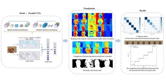
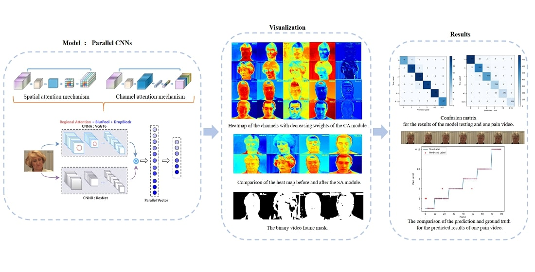
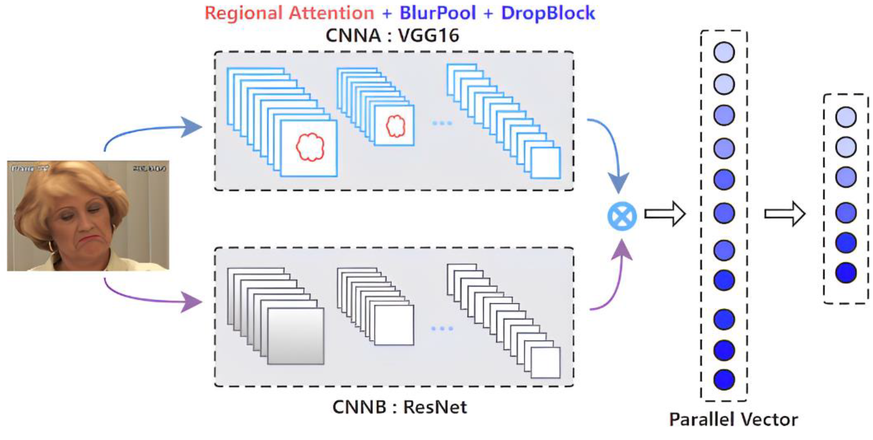
3.1. Parallel CNNs
3.2. Insertion of the Attention Mechanism
3.2.1. Spatial Attention
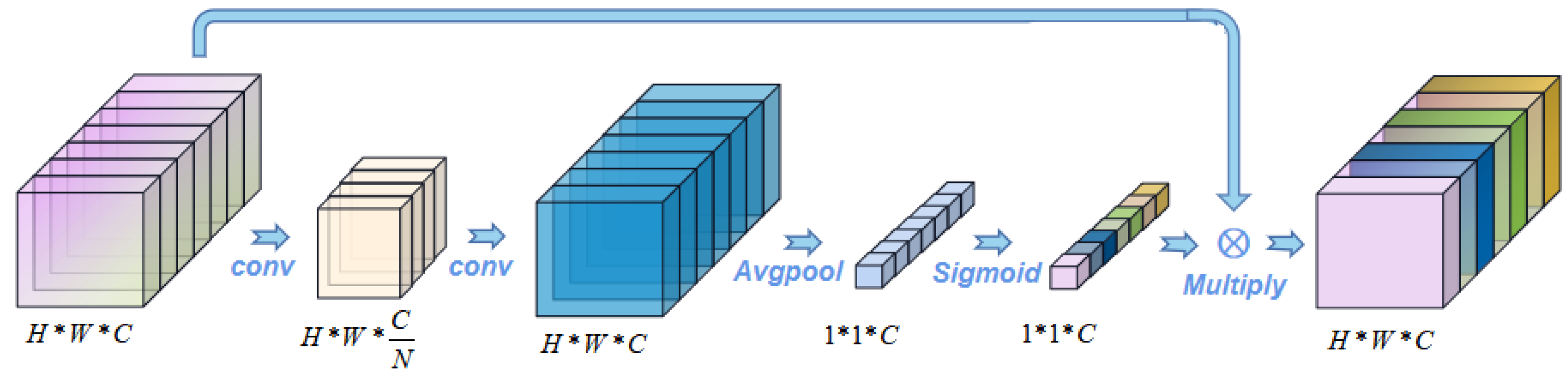
3.2.2. Channel Attention
3.3. Enhancement of Features
- The selection of low-correlation channels;
- The segmentation of regions with low correlation;
- The enhancement of the high-correlation features.
3.3.1. Selection of Low-Correlation Channels
3.3.2. Segmentation of Regions with Low Correlation
3.3.3. Enhancement of the High-Correlation Features
| Algorithm 1:Mask Generation Based on DropBlock |
| Input: |
|
4. Experiments
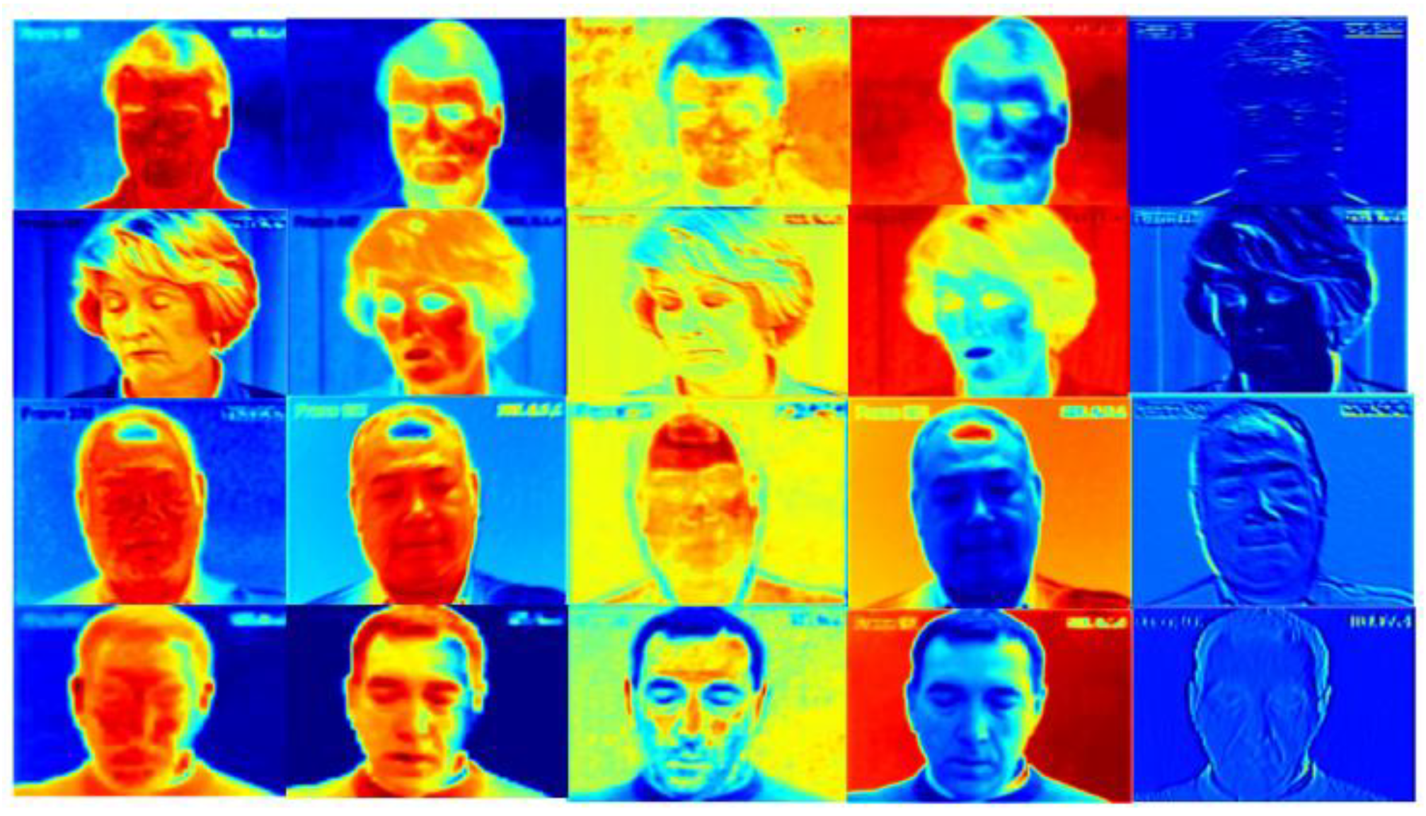
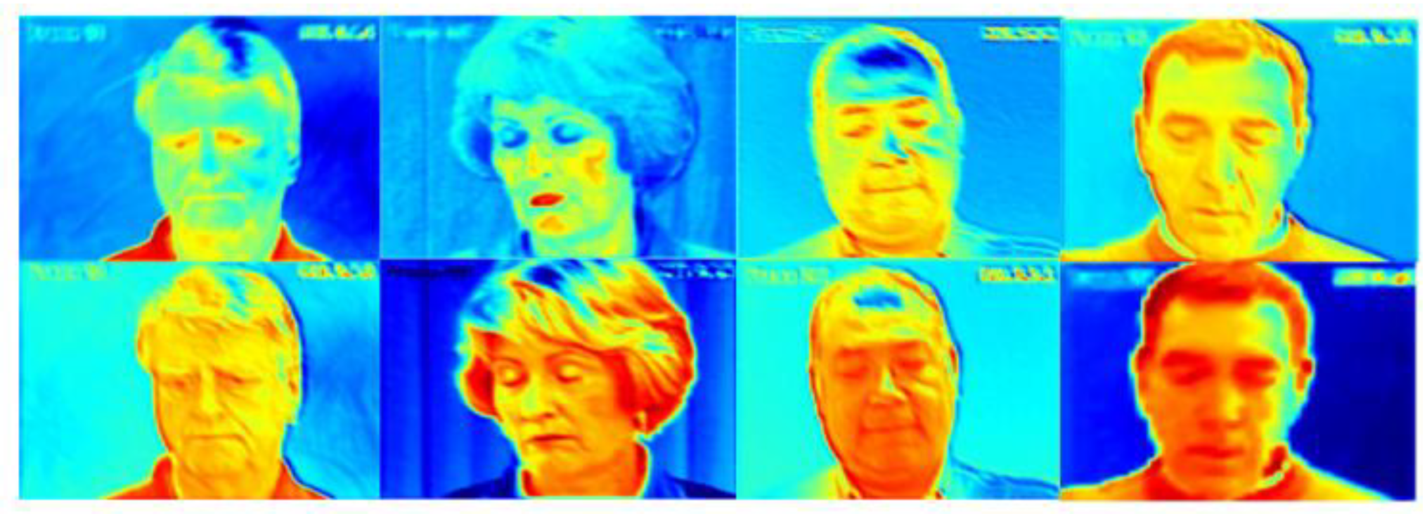
4.1. Preparation of UNBC
4.2. Experiment on UNBC
4.2.1. Ablation of the Attention Modules in the CNNA
4.2.2. Ablation of the Model Structure
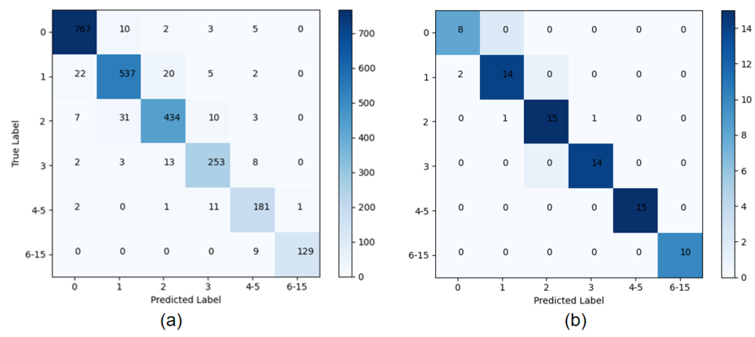
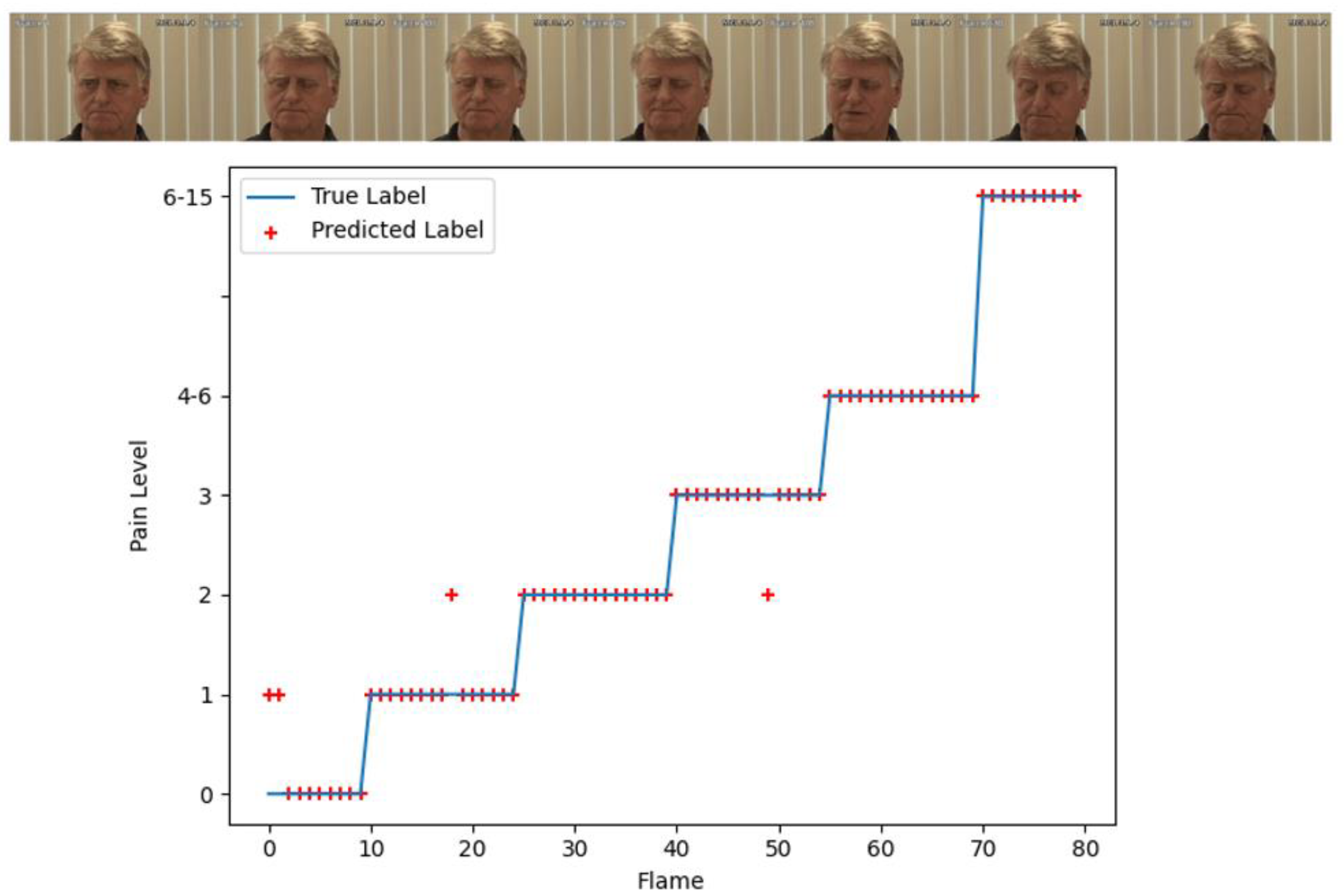
4.2.3. Comparison with Other State-of-the-Art Methods
5. Conclusions
Author Contributions
Funding
Informed Consent Statement
Data Availability Statement
Conflicts of Interest
References
- Raja, S.N.; Carr, D.B.; Cohen, M.; Finnerup, N.B.; Flor, H.; Gibson, S.; Keefe, F.J.; Mogil, J.S.; Ringkamp; Sluka, K.A.; et al. The revised International Association for the Study of Pain definition of pain: Concepts, challenges, and compromises. Pain 2020. Publish Ahead of Print. [Google Scholar]
- Morone, N.E.; Weiner, D.K. Pain as the fifth vital sign: Exposing the vital need for pain education. Clin. Ther. 2013, 35, 1728–1732. [Google Scholar] [CrossRef] [PubMed] [Green Version]
- Ferreira-Valente, M.A.; Pais-Ribeiro, J.L.; Jensen, M.P. Validity of four pain intensity rating scales. Pain 2011, 152, 2399–2404. [Google Scholar] [CrossRef] [PubMed]
- Pozza, D.H.; Azevedo, L.F.; Lopes, J.M.C. Pain as the fifth vital sign—A comparison between public and private healthcare systems. PLoS ONE 2021, 16, e0259535. [Google Scholar] [CrossRef] [PubMed]
- Copot, D.; Ionescu, C. Models for Nociception Stimulation and Memory Effects in Awake and Aware Healthy Individuals. IEEE Trans. Biomed. Eng. 2019, 66, 718–726. [Google Scholar] [CrossRef]
- Haddad, W.M.; Bailey, J.M.; Hayakawa, T.; Hovakimyan, N. Neural network adaptive output feedback control for intensive care unit sedation and intraoperative anesthesia. IEEE Trans. Neural Netw. 2007, 18, 1049–1066. [Google Scholar] [CrossRef]
- Desbiens, N.A.; Wu, A.W.; Broste, S.K.; Wenger, N.S.; Connors, A.F., Jr.; Lynn, J.; Yasui, Y.; Phillips, R.S.; Fulkerson, W. Pain and satisfaction with pain control in seriously ill hospitalized adults: Findings from the SUPPORT research investigations. For the SUPPORT investigators. Study to understand prognoses and preferences for outcomes and risks of treatment. Crit. Care Med. 1996, 24, 1953–1961. [Google Scholar] [CrossRef]
- McArdle, P. Intravenous analgesia. Crit. Care Clin. 1999, 15, 89–104. [Google Scholar] [CrossRef]
- Ionescu, C.M.; Copot, D.; Keyser, R.D. Anesthesiologist in the Loop and Predictive Algorithm to Maintain Hypnosis While Mimicking Surgical Disturbance. IFAC-PapersOnLine 2017, 50, 15080–15085. [Google Scholar] [CrossRef]
- Gordon, D.B. Acute pain assessment tools: Let us move beyond simple pain ratings. Curr. Opin. Anaesthesiol. 2015, 28, 565–569. [Google Scholar] [CrossRef]
- Ekman, P.E.; Friesen, W.V. Facial Action Coding System: A Technique for the Measurement of Facial Movement; Consulting Psychologists Press: Palo Alto, CA, USA, 1978. [Google Scholar]
- Prkachin, K.M.; Solomon, P.E. The structure, reliability and validity of pain expression: Evidence from patients with shoulder pain. Pain 2008, 139, 267–274. [Google Scholar] [CrossRef]
- Ashraf, A.B.; Lucey, S.; Cohn, J.F.; Chen, T.; Ambadar, Z.; Prkachin, K.M.; Solomon, P.E. The Painful Face—Pain Expression Recognition Using Active Appearance Models. Image Vis. Comput. 2009, 27, 1788–1796. [Google Scholar] [CrossRef] [PubMed] [Green Version]
- Lucey, P.; Cohn, J.F.; Matthews, I.; Lucey, S.; Sridharan, S.; Howlett, J.; Prkachin, K.M. Automatically Detecting Pain in Video Through Facial Action Units. IEEE Trans. Syst. Man Cybern. Part B 2011, 41, 664–674. [Google Scholar] [CrossRef] [PubMed]
- Khan, R.A.; Meyer, A.; Konik, H.; Bouakaz, S. Pain Detection Through Shape and Appearance Features. In Proceedings of the IEEE International Conference on Multimedia & Expo, San Jose, CA, USA, 15–19 July 2013. [Google Scholar]
- Zhao, R.; Gan, Q.; Wang, S.; Ji, Q. Facial Expression Intensity Estimation Using Ordinal Information. In Proceedings of the Computer Vision & Pattern Recognition, Las Vegas, NV, USA, 27–30 June 2016. [Google Scholar]
- Wang, F.; Xiang, X.; Liu, C.; Tran, T.D.; Reiter, A.; Hager, G.D.; Quon, H.; Cheng, J.; Yuille, A.L. Regularizing Face Verification Nets for Pain Intensity Regression. In Proceedings of the IEEE International Conference on Image Processing, Beijing, China, 17–20 September 2017. [Google Scholar]
- Zhou, J.; Hong, X.; Su, F.; Zhao, G. Recurrent Convolutional Neural Network Regression for Continuous Pain Intensity Estimation in Video. In Proceedings of the IEEE Conference on Computer Vision & Pattern Recognition Workshops, Las Vegas, NV, USA, 26 June–1 July 2016. [Google Scholar]
- Rodriguez, P.; Cucurull, G.; Gonalez, J.; Gonfaus, J.M.; Nasrollahi, K.; Moeslund, T.B.; Roca, F.X. Deep Pain: Exploiting Long Short-Term Memory Networks for Facial Expression Classification. IEEE Trans. Cybern. 2022, 52, 3314–3324. [Google Scholar] [CrossRef] [PubMed] [Green Version]
- Tavakolian, M.; Hadid, A. A Spatiotemporal Convolutional Neural Network for Automatic Pain Intensity Estimation from Facial Dynamics. Int. J. Comput. Vis. 2019, 127, 1413–1425. [Google Scholar] [CrossRef] [Green Version]
- Wang, J.; Sun, H. Pain Intensity Estimation Using Deep Spatiotemporal and Handcrafted Features. IEICE Trans. Inf. Syst. 2018, E101.D, 1572–1580. [Google Scholar] [CrossRef] [Green Version]
- Tavakolian, M.; Lopez, M.B.; Liu, L. Self-supervised Pain Intensity Estimation from Facial Videos via Statistical Spatiotemporal Distillation. Pattern Recognit. Lett. 2020, 140, 26–33. [Google Scholar] [CrossRef]
- Xin, X.; Lin, X.; Yang, S.; Zheng, X. Pain intensity estimation based on a spatial transformation and attention CNN. PLoS ONE 2020, 15, e0232412. [Google Scholar] [CrossRef]
- Huang, D.; Xia, Z.; Mwesigye, J.; Feng, X. Pain-attentive network: A deep spatio-temporal attention model for pain estimation. Multimed. Tools Appl. 2020, 79, 28329–28354. [Google Scholar] [CrossRef]
- Huang, Y.; Qing, L.; Xu, S.; Wang, L.; Peng, Y. HybNet: A hybrid network structure for pain intensity estimation. Vis. Comput. 2022, 38, 871–882. [Google Scholar] [CrossRef]
- Ghiasi, G.; Lin, T.-Y.; Le, Q.V. DropBlock: A regularization method for convolutional networks. In Proceedings of the 32nd International Conference on Neural Information Processing Systems, Montreal, Canada, 2–8 December 2018. [Google Scholar]
- Krizhevsky, A.; Sutskever, I.; Hinton, G.E. ImageNet Classification with Deep Convolutional Neural Networks. Commun. ACM. 2017, 60, 84–90. [Google Scholar] [CrossRef] [Green Version]
- Simonyan, K.; Zisserman, A. Very Deep Convolutional Networks for Large-Scale Image Recognition. arXiv 2014, arXiv:1409.1556. [Google Scholar]
- Szegedy, C.; Liu, W.; Jia, Y.; Sermanet, P.; Reed, S.; Anguelov, D.; Erhan, D.; Vanhoucke, V.; Rabinovich, A. Going Deeper with Convolutions. In Proceedings of the IEEE Conference on Computer Vision and Pattern Recognition, Boston, MA, USA, 7–12 June 2015. [Google Scholar]
- He, K.; Zhang, X.; Ren, S.; Sun, J. Deep Residual Learning for Image Recognition. In Proceedings of the 2016 IEEE Conference on Computer Vision and Pattern Recognition (CVPR), Las Vegas, NV, USA, 27–30 June 2016. [Google Scholar]
- Parkhi, O.M.; Vedaldi, A.; Zisserman, A. Deep Face Recognition. In Proceedings of the British Machine Vision Conference, Swansea, UK, 7–10 September 2015. [Google Scholar]
- Liu, W.; Wen, Y.; Yu, Z.; Li, M.; Raj, B.; Song, L. SphereFace: Deep Hypersphere Embedding for Face Recognition. In Proceedings of the 2017 IEEE Conference on Computer Vision and Pattern Recognition (CVPR), Honolulu, HI, USA, 21–26 July 2017. [Google Scholar]
- Gao, Q.; Liu, J.; Ju, Z.; Li, Y.; Zhang, T.; Zhang, L. Static Hand Gesture Recognition with Parallel CNNs for Space Human-Robot Interaction. In Intelligent Robotics and Applications; Springer: Cham, Switzerland, 2017. [Google Scholar]
- Wang, C.; Shi, J.; Zhang, Q.; Ying, S. Histopathological image classification with bilinear convolutional neural networks. In Proceedings of the 39th Annual International Conference of the IEEE Engineering in Medicine and Biology Society (EMBC), Jeju, Republic of Korea, 11–15 July 2017. [Google Scholar]
- Chowdhury, A.R.; Lin, T.Y.; Maji, S.; Learned-Miller, E. One-to-many face recognition with bilinear CNNs. In Proceedings of the IEEE Winter Conference on Applications of Computer Vision (WACV), Lake Placid, NY, USA, 7–10 March 2016. [Google Scholar]
- Yang, S.; Peng, G. Parallel Convolutional Networks for Image Recognition via a Discriminator. In Computer Vision—ACCV 2018; Springer: Cham, Switzerland, 2019. [Google Scholar]
- Zhang, C.; He, D.; Li, Z.; Wang, Z. Parallel Connecting Deep and Shallow CNNs for Simultaneous Detection of Big and Small Objects. In Pattern Recognition and Computer Vision; Springer: Cham, Switzerland, 2018. [Google Scholar]
- Schneider, W.E.; Shiffrin, R.M. Controlled and automatic human information processing: I. Detection, search, and attention. Psychol. Rev. 1977, 84, 1–66. [Google Scholar] [CrossRef]
- Fu, J.; Liu, J.; Tian, H.; Li, Y.; Bao, Y.; Fang, Z.; Ku, H. Dual Attention Network for Scene Segmentation. In Proceedings of the 2019 IEEE/CVF Conference on Computer Vision and Pattern Recognition (CVPR), Long Beach, CA, USA, 15–20 June 2019. [Google Scholar]
- Chattopadhyay, S.; Basak, H. Multi-scale Attention U-Net (MsAUNet): A Modified U-Net Architecture for Scene Segmentation. arXiv 2020, arXiv:2009.06911. [Google Scholar]
- Yang, Z.; Liu, Q.; Liu, G. Better Understanding: Stylized Image Captioning with Style Attention and Adversarial Training. Symmetry 2020, 12, 1978. [Google Scholar] [CrossRef]
- Li, K.; Wu, Z.; Peng, K.C.; Ernst, J.; Fu, Y. Tell Me Where to Look: Guided Attention Inference Network. In Proceedings of the 2018 IEEE/CVF Conference on Computer Vision and Pattern Recognition, Salt Lake City, UT, USA, 18–23 June 2018. [Google Scholar]
- Peng, Y.; He, X.; Zhao, J. Object-Part Attention Model for Fine-grained Image Classification. IEEE Trans. Image Process. A Publ. IEEE Signal Process. Soc. 2017, 27, 1487–1500. [Google Scholar] [CrossRef] [Green Version]
- Xiao, T.; Xu, Y.; Yang, K.; Zhang, J.; Peng, Y.; Zhang, Z. The Application of Two-level Attention Models in Deep Convolutional Neural Network for Fine-grained Image Classification. In Proceedings of the IEEE Conference on Computer Vision and Pattern Recognition (CVPR), Boston, MA, USA, 7–12 June 2015. [Google Scholar]
- Xie, C.; Liu, S.; Li, C.; Cheng, M.; Zuo, W.; Liu, X.; Wen, S.; Ding, E. Image Inpainting with Learnable Bidirectional Attention Maps. In Proceedings of the IEEE/CVF International Conference on Computer Vision (ICCV), Seoul, Korea, 27 October–2 November 2019. [Google Scholar]
- Yu, J.; Lin, Z.; Yang, J.; Shen, X.; Lu, X.; Huang, T.S. Generative Image Inpainting with Contextual Attention. In Proceedings of the IEEE Conference on Computer Vision and Pattern Recognition (CVPR), Salt Lake City, UT, USA, 18–23 June 2018. [Google Scholar]
- Woo, S.; Park, J.; Lee, J.Y.; Kweon, I.S. CBAM: Convolutional Block Attention Module. In Computer Vision—ECCV 2018; Springer: Cham, Switzerland, 2018. [Google Scholar]
- Chen, J.; Chen, Y.; Li, W.; Ning, G.; Tong, M.; Hilton, A. Channel and spatial attention based deep object co-segmentation. In Knowledge Based Systems; Elsevier: Amsterdam, The Netherlands, 2021; Volume 211, p. 106550. [Google Scholar]
- Liao, S.; Liu, H.; Yang, J.; Ge, Y. A channel-spatial-temporal attention-based network for vibration-based damage detection. Inf. Sci. 2022, 606, 213–229. [Google Scholar] [CrossRef]
- Karthik, R.; Menaka, R.; Siddharth, M.V. Classification of breast cancer from histopathology images using an ensemble of deep multiscale networks. Biocybern. Biomed. Eng. 2022, 42, 963–976. [Google Scholar] [CrossRef]
- Gohil, S.; Lad, A. Kidney and Kidney Tumor Segmentation Using Spatial and Channel Attention Enhanced U-Net. In Proceedings of the Kidney and Kidney Tumor Segmentation: MICCAI 2021 Challenge, Strasbourg, France, 27 September 2021. [Google Scholar]
- Chinnappa, G.; Rajagopal, M.K. Residual attention network for deep face recognition using micro-expression image analysis. J. Ambient. Intell. Humaniz. Comput. 2021, 13, 117. [Google Scholar] [CrossRef]
- Wang, J.; Yuan, Y.; Yu, G. Face Attention Network: An Effective Face Detector for the Occluded Faces. arXiv 2017, arXiv:1711.07246. [Google Scholar]
- Lucey, P.; Cohn, J.F.; Prkachin, K.M.; Solomon, P.E.; Matthews, I. Painful data: The UNBC-McMaster shoulder pain expression archive database. In Proceedings of the Ninth IEEE International Conference on Automatic Face and Gesture Recognition (FG 2011), Santa Barbara, CA, USA, 21–25 March 2011. [Google Scholar]
- Roychowdhury, A.; Maji, S.; Lin, T.Y. Bilinear CNNs for Fine-grained Visual Recognition. IEEE Trans. Pattern Anal. Mach. Intell. 2017, 40, 1309–1322. [Google Scholar]
- Azulay, A.; Weiss, Y. Why do deep convolutional networks generalize so poorly to small image transformations? arXiv 2018, arXiv:1805.12177. [Google Scholar]
- Engstrom, L.; Tran, B.; Tsipras, D.; Schmidt, L.; Madry, A. Exploring the Landscape of Spatial Robustness. arXiv 2017, arXiv:1712.02779. [Google Scholar]
- Zhang, R. Making Convolutional Networks Shift-Invariant Again. arXiv 2019, arXiv:1904.11486. [Google Scholar]
- Selvaraju, R.R.; Cogswell, M.; Das, A.; Vedantam, R.; Parikh, D.; Batra, D. Grad-CAM: Visual Explanations from Deep Networks via Gradient-Based Localization. In Proceedings of the International Conference on Computer Vision, Venice, Italy, 22–29 October 2017. [Google Scholar]
- Hinton, G.E.; Srivastava, N.; Krizhevsky, A.; Sutskever, I.; Salakhutdinov, R. Improving neural networks by preventing co-adaptation of feature detectors. Comput. Sci. 2012, 3, 212–223. [Google Scholar]
- Kaltwang, S.; Rudovic, O.; Pantic, M. Continuous Pain Intensity Estimation from Facial Expressions. In Advances in Visual Computing; Springer: Berlin/Heidelberg, Germany, 2012. [Google Scholar]
- Florea, C.; Florea, L.; Vertan, C. Learning Pain from Emotion: Transferred HoT Data Representation for Pain Intensity Estimation. In Computer Vision—ECCV 2014 Workshops; Springer: Cham, Switzerland, 2014. [Google Scholar]
- Zhang, Y.; Zhao, R.; Dong, W.; Hu, B.G.; Ji, Q. Bilateral Ordinal Relevance Multi-Instance Regression for Facial Action Unit Intensity Estimation. In Proceedings of the 2018 IEEE/CVF Conference on Computer Vision and Pattern Recognition (CVPR), Salt Lake City, UT, USA, 18–22 June 2018. [Google Scholar]


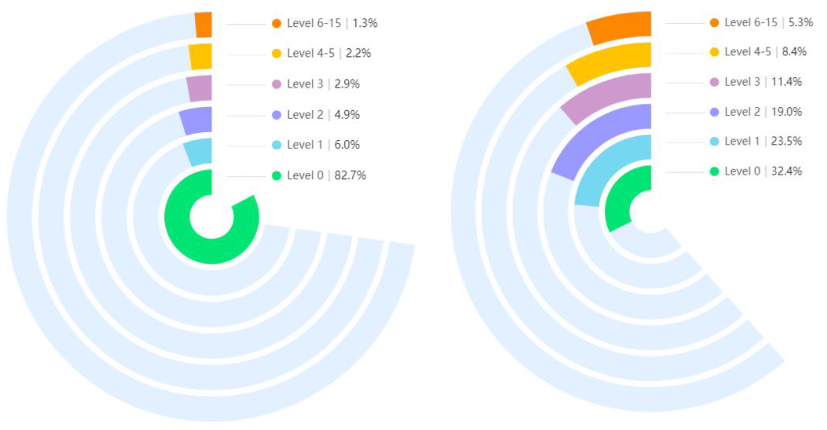
| PSPI Score | Total Frames | Frequency | Frequency After Clustering |
|---|---|---|---|
| 0 | 40,029 | 82.7439% | 82.7439% |
| 1 | 2909 | 6.0132% | 6.0132% |
| 2 | 2351 | 4.8597% | 4.8597% |
| 3 | 1412 | 2.9187% | 2.9187% |
| 4 | 802 | 1.6578% | 2.1581% |
| 5 | 242 | 0.5002% | |
| 6 | 270 | 0.5581% | 1.3498% |
| 7 | 53 | 0.1096% | |
| 8 | 79 | 0.1633% | |
| 9 | 32 | 0.0661% | |
| 10 | 67 | 0.1385% | |
| 11 | 76 | 0.1571% | |
| 12 | 48 | 0.0992% | |
| 13 | 22 | 0.0455% | |
| 14 | 1 | 0.0021% | |
| 15 | 5 | 0.0103% |
| Attention Combination | RMSE | PCC |
|---|---|---|
| CA | 1.02 | 0.74 |
| SA | 1.13 | 0.68 |
| CA–SA | 0.73 | 0.85 |
| SA–CA | 0.91 | 0.75 |
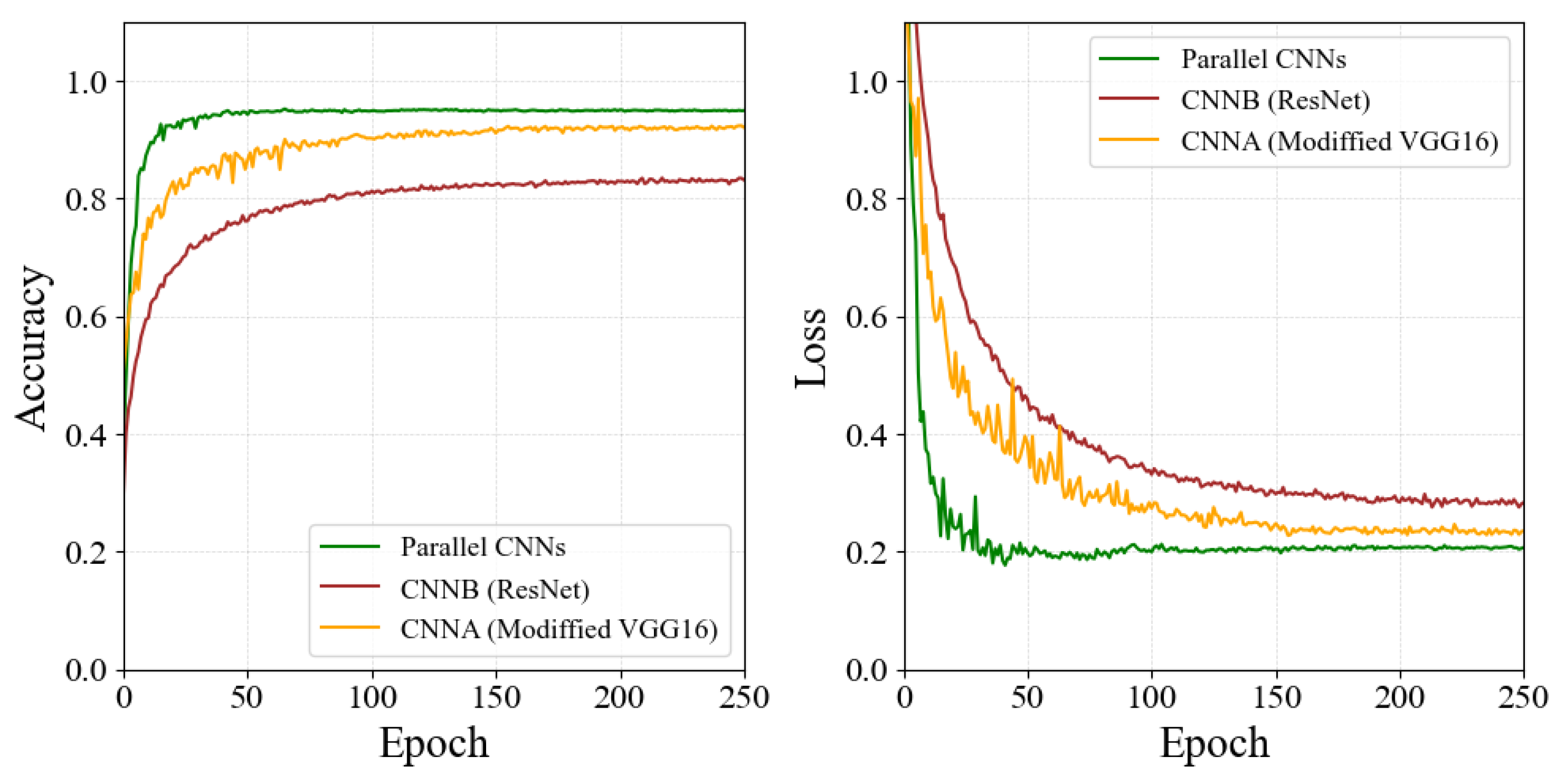
| Model Combination | RMSE | PCC |
|---|---|---|
| CNNA: Modified VGG16 | 0.73 | 0.85 |
| CNNB: ResNet | 1.15 | 0.67 |
| Parallel structure (Ours) | 0.45 | 0.96 |
Publisher’s Note: MDPI stays neutral with regard to jurisdictional claims in published maps and institutional affiliations. |
© 2022 by the authors. Licensee MDPI, Basel, Switzerland. This article is an open access article distributed under the terms and conditions of the Creative Commons Attribution (CC BY) license (https://creativecommons.org/licenses/by/4.0/).
Share and Cite
Ye, X.; Liang, X.; Hu, J.; Xie, Y. Image-Based Pain Intensity Estimation Using Parallel CNNs with Regional Attention. Bioengineering 2022, 9, 804. https://doi.org/10.3390/bioengineering9120804
Ye X, Liang X, Hu J, Xie Y. Image-Based Pain Intensity Estimation Using Parallel CNNs with Regional Attention. Bioengineering. 2022; 9(12):804. https://doi.org/10.3390/bioengineering9120804
Chicago/Turabian StyleYe, Xinting, Xiaokun Liang, Jiani Hu, and Yaoqin Xie. 2022. "Image-Based Pain Intensity Estimation Using Parallel CNNs with Regional Attention" Bioengineering 9, no. 12: 804. https://doi.org/10.3390/bioengineering9120804