

GIT-Net: An Ensemble Deep Learning-Based GI Tract Classification of Endoscopic Images
 , , , and
Abstract
:
1. Introduction
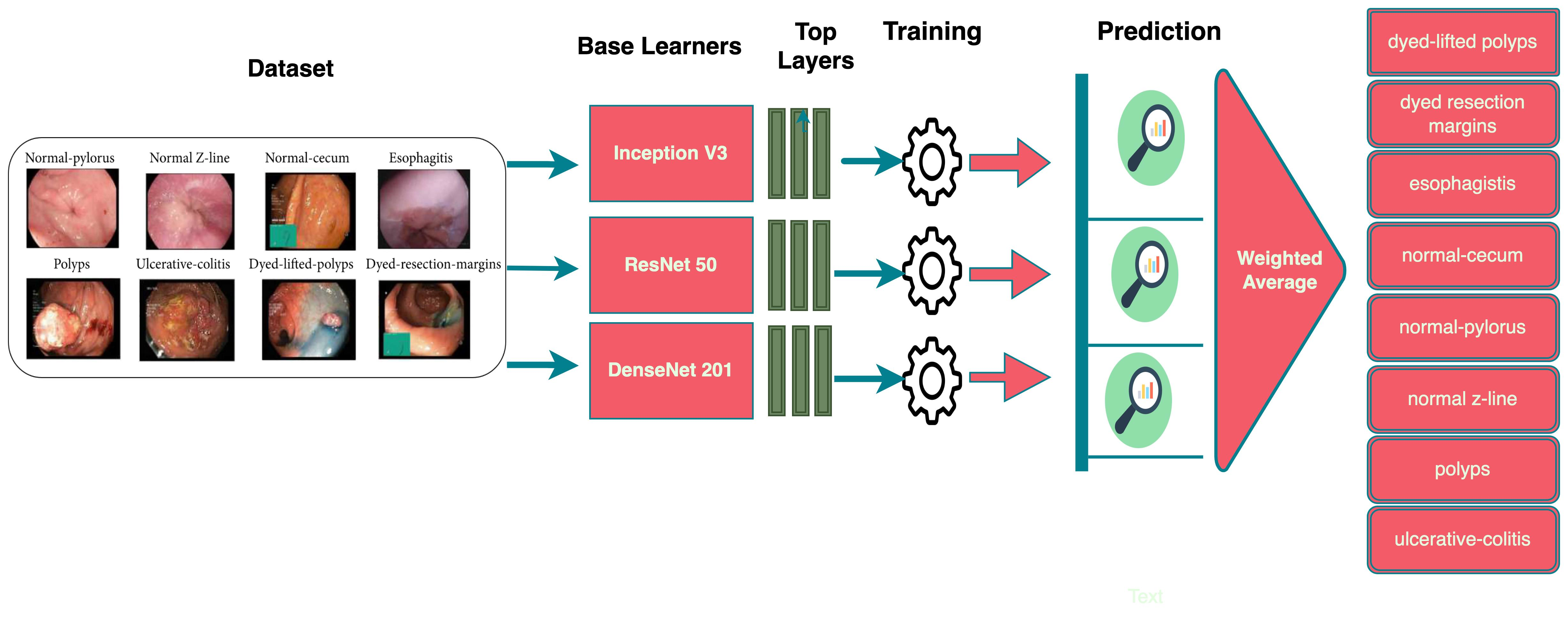
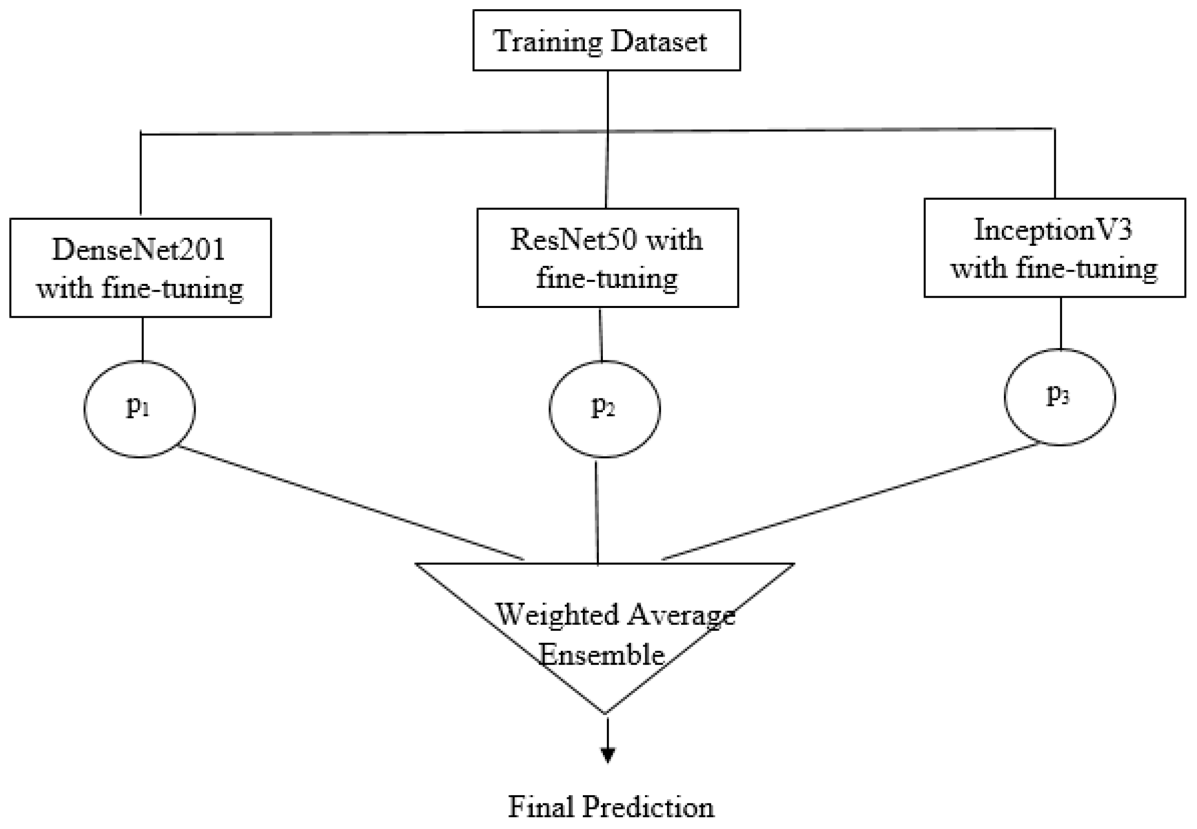
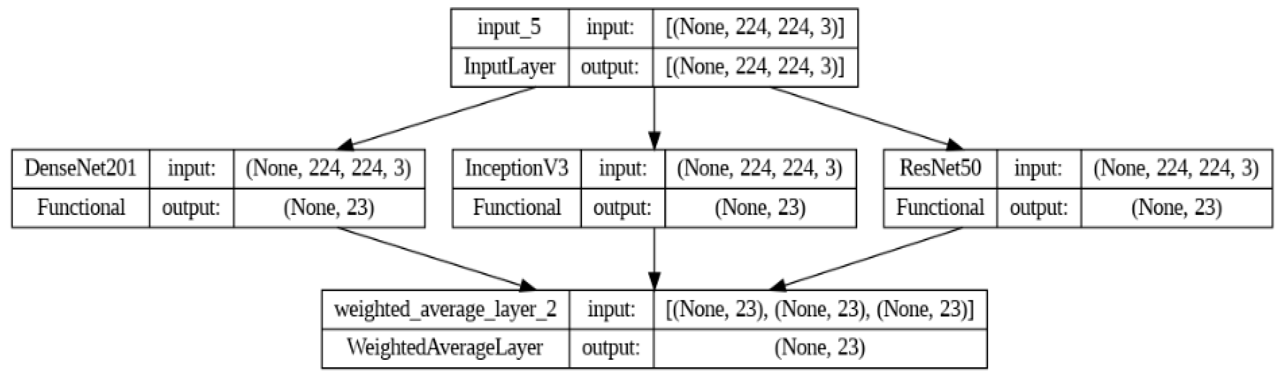
- We propose a deep ensemble model with three fine-tuned base learners, namely ResNet50, DenseNet201, and InceptionV3.
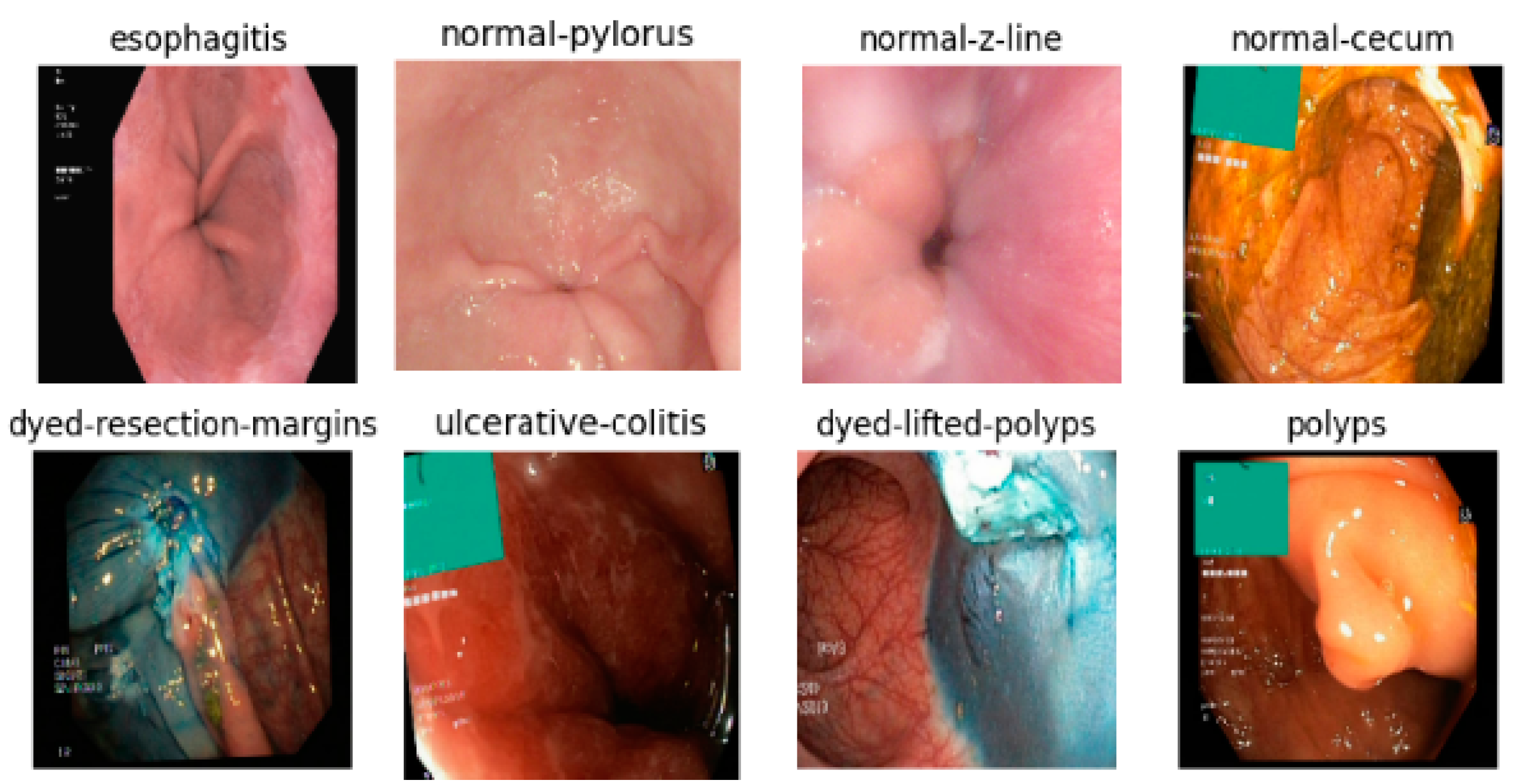
- The proposed approach is evaluated on the KVASIR v2 dataset, consisting of eight classes with 8000 samples.
- We conducted extensive experiments to show significant improvement in accuracy, precision, and recall of the ensemble model compared to the baseline models.
2. Literature Review
3. Dataset
4. Methods and Techniques
4.1. Transfer Learning
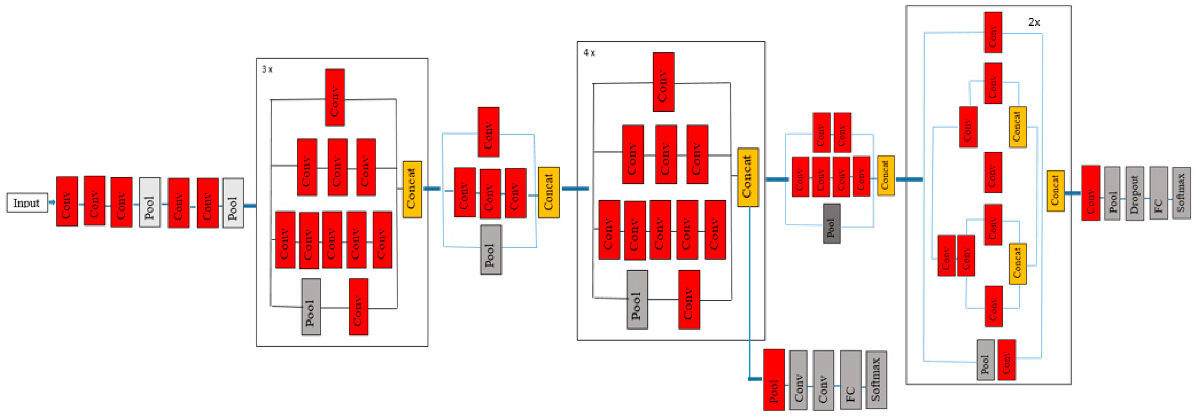
4.2. InceptionV3 Model
- Larger convolution layers are factored into small convolution layers.
- More factorization is performed by adding asymmetric convolutions of the form n × 1.
- Auxiliary classifiers are added to improve the convergence of the network.
- The activation dimensions of the network filters are expanded to reduce the grid size of the model.
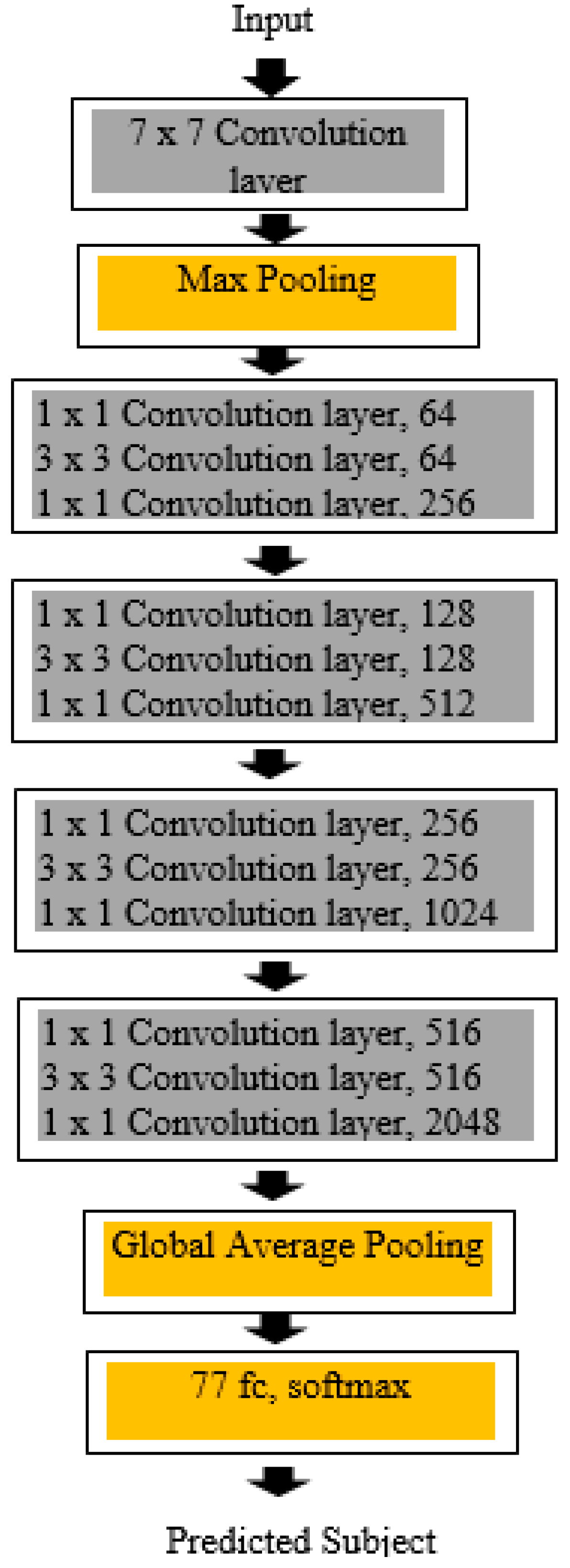
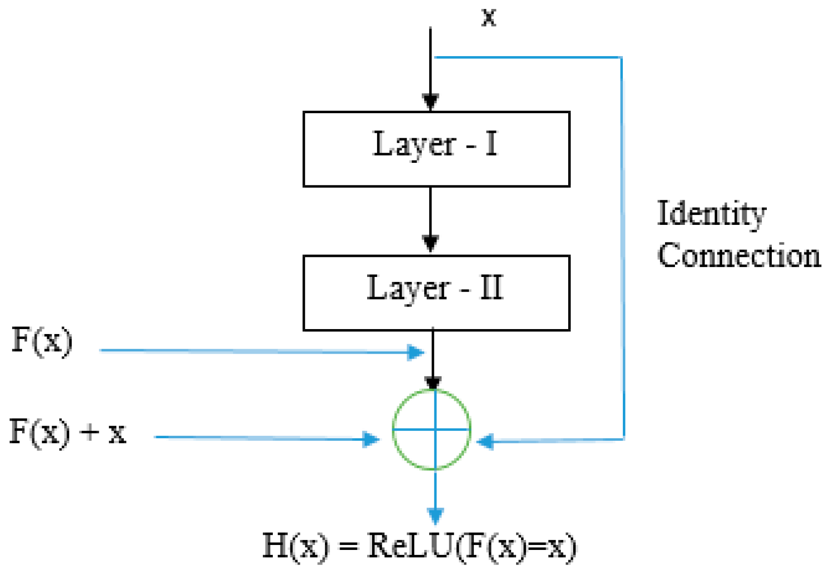
4.3. ResNet50 Model
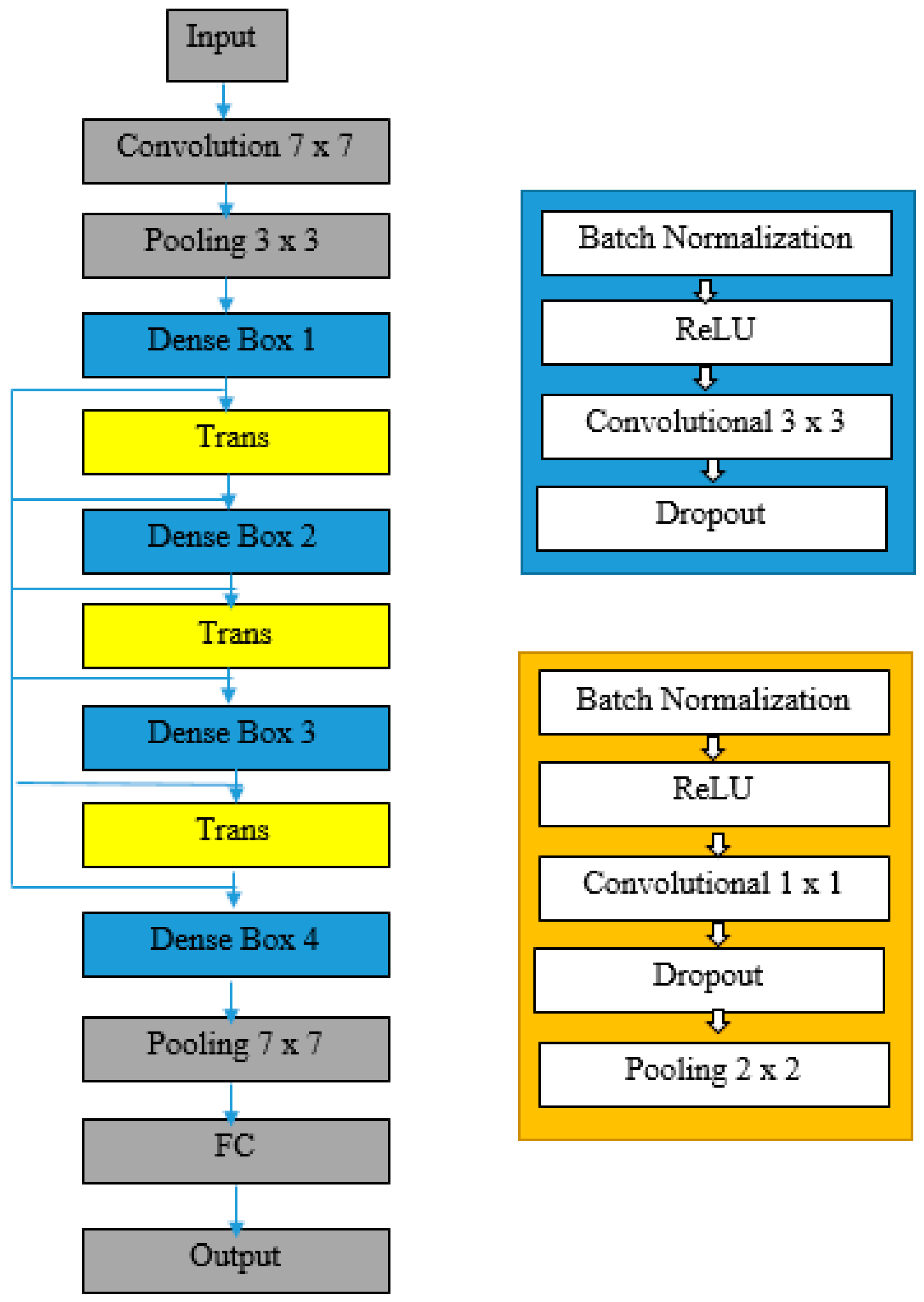
4.4. DenseNet201 Model
5. Proposed Ensemble Model
- Model Averaging Ensemble;
- Weighted Averaging Ensemble;
- Stacking Ensemble, etc.
5.1. Model Averaging Ensemble
5.2. Weighted Averaging Ensemble
5.3. Stacking Ensemble
6. Experiments
- True Positive (TP).
- True Negative (TN).
- False Positive (FP).
- False Negative (FN).
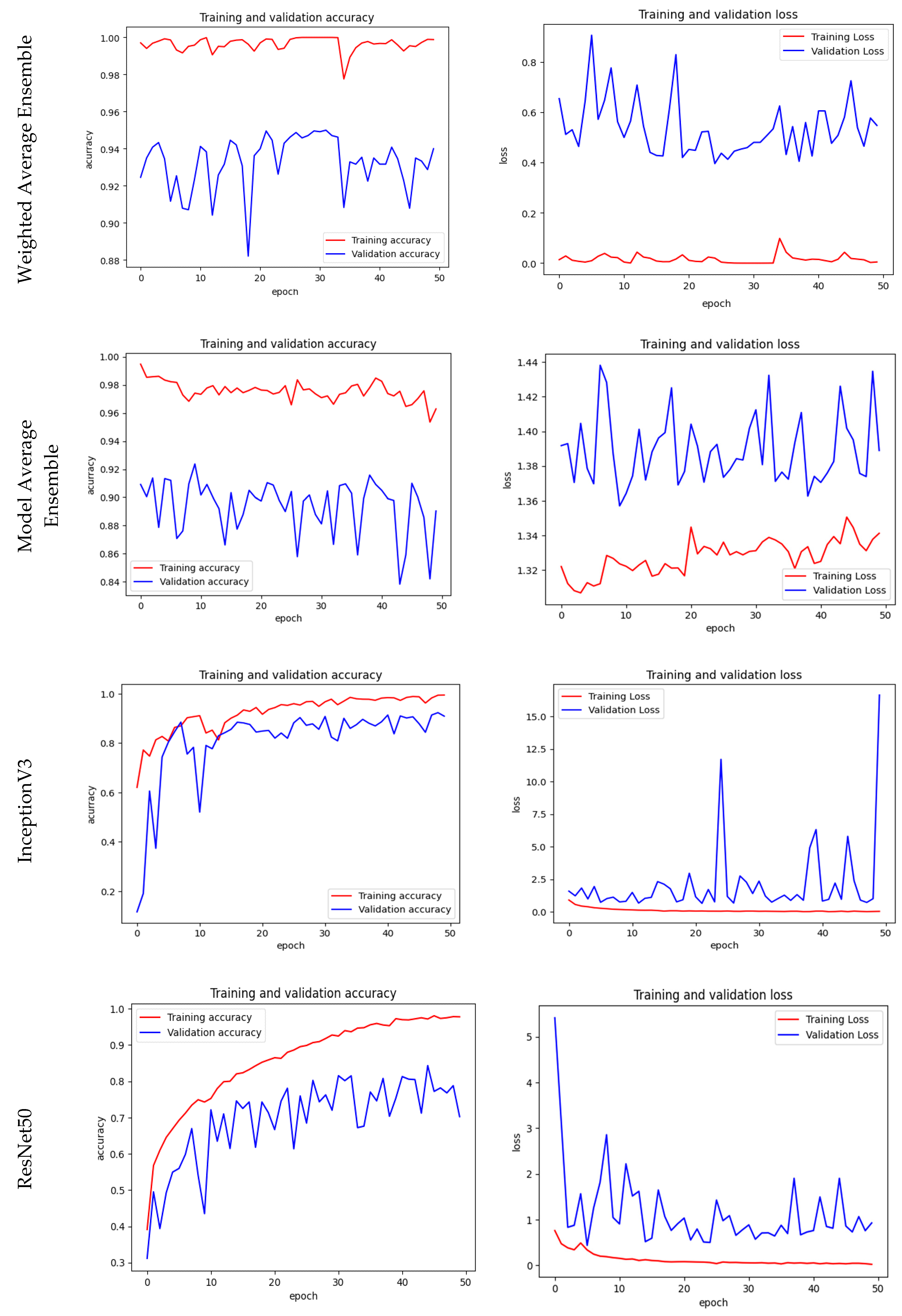
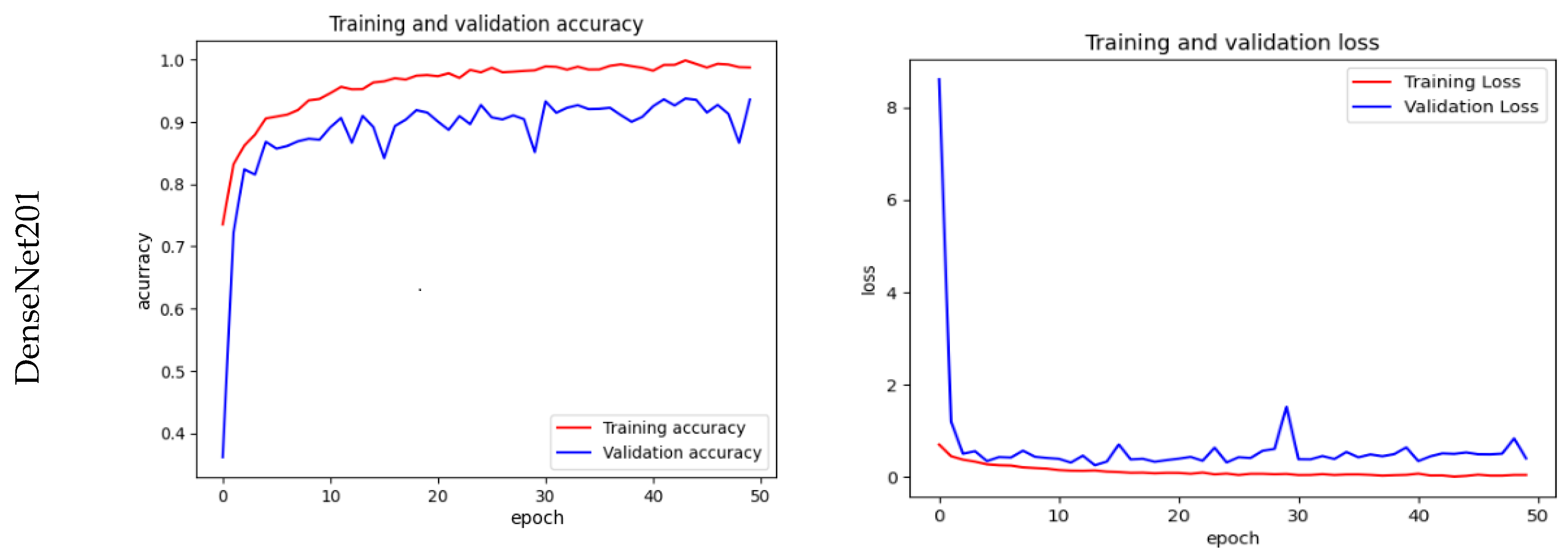
Training, Validation Accuracy & Loss
7. Discussion
8. Conclusions
Author Contributions
Funding
Institutional Review Board Statement
Data Availability Statement
Conflicts of Interest
References
- Al-Adhaileh, M.H.; Senan, E.M.; Alsaade, F.W.; Aldhyani, T.H.H.; Alsharif, N.; Alqarni, A.A.; Uddin, M.I.; Alzahrani, M.Y.; Alzain, E.D.; Jadhav, M.E. Deep Learning Algorithms for Detection and Classification of Gastrointestinal Diseases. Complexity 2021, 2021, 6170416. [Google Scholar] [CrossRef]
- Dawoodi, S.; Dawoodi, I.; Dixit, P. Gastrointestinal problem among Indian adults: Evidence from longitudinal aging study in India 2017-18. Front. Public Health 2022, 10, 911354. [Google Scholar] [CrossRef]
- Ramamurthy, K.; George, T.T.; Shah, Y.; Sasidhar, P. A Novel Multi-Feature Fusion Method for Classification of Gastrointestinal Diseases Using Endoscopy Images. Diagnostics 2022, 12, 2316. [Google Scholar] [CrossRef]
- Naz, J.; Sharif, M.; Yasmin, M.; Raza, M.; Khan, M.A.J. Detection and Classification of Gastrointestinal Diseases Using Machine Learning. Curr. Med. Imaging 2021, 17, 479–490. [Google Scholar] [CrossRef]
- Pogorelov, K.; Randel, K.R.; Griwodz, C.; Eskeland, S.L.; de Lange, T.; Johansen, D.; Spampinato, C.; Dang-Nguyen, D.-T.; Lux, M.; Schmidt, P.T.; et al. KVASIR: A multi-class image dataset for computer-aided gastrointestinal disease detection. In Proceedings of the 8th ACM on Multimedia Systems Conference, New York, NY, USA, 20–23 June 2017; pp. 164–169. [Google Scholar] [CrossRef] [Green Version]
- Adadi, A.; Adadi, S.; Berrada, M. Gastroenterology Meets Machine Learning: Status Quo and Quo Vadis. Adv. Bioinform. 2019, 2019, 1870975. [Google Scholar] [CrossRef] [PubMed] [Green Version]
- Su, Q.; Wang, F.; Chen, D.; Chen, G.; Li, C.; Wei, L. Deep convolutional neural networks with ensemble learning and transfer learning for automated detection of gastrointestinal diseases. Comput. Biol. Med. 2022, 150, 106054. [Google Scholar] [CrossRef] [PubMed]
- Ramzan, M.; Raza, M.; Sharif, M.; Khan, M.A.; Nam, Y. Gastrointestinal Tract Infections Classification Using Deep Learning. Comput. Mater. Contin. 2021, 69, 3239–3257. [Google Scholar] [CrossRef]
- Ali, S.; Dmitrieva, M.; Ghatwary, N.; Bano, S.; Polat, G.; Temizel, A.; Krenzer, A.; Hekalo, A.; Guo, Y.B.; Matuszewski, B.; et al. Deep learning for detection and segmentation of artifact and disease instances in gastrointestinal endoscopy. Med. Image Anal. 2021, 70, 102002. [Google Scholar] [CrossRef] [PubMed]
- Zhou, J.; Hu, N.; Huang, Z.Y.; Song, B.; Wu, C.C.; Zeng, F.X.; Wu, M. Application of artificial intelligence in gastrointestinal disease: A narrative review. Ann. Transl. Med. 2021, 9, 1188. [Google Scholar] [CrossRef]
- Haile, M.B.; Salau, A.O.; Enyew, B.; Belay, A.J. Detection and classification of gastrointestinal disease using convolutional neural network and SVM. Cogent Eng. 2022, 9, 2084878. [Google Scholar] [CrossRef]
- Yogapriya, J.; Chandran, V.; Sumithra, M.G.; Anitha, P.; Jenopaul, P.; Dhas, C.S.G. Gastrointestinal Tract Disease Classification from Wireless Endoscopy Images Using Pretrained Deep Learning Model. Comput. Math. Methods Med. 2021, 2021, 5940433. [Google Scholar] [CrossRef]
- Lonseko, Z.M.; Adjei, P.E.; Du, W.; Luo, C.; Hu, D.; Zhu, L.; Gan, T.; Rao, N. Gastrointestinal Disease Classification in Endoscopic Images Using Attention-Guided Convolutional Neural Networks. Appl. Sci. 2021, 11, 11136. [Google Scholar] [CrossRef]
- Khan, M.A.; Khan, M.A.; Ahmed, F.; Mittal, M.; Goyal, L.M.; Hemanth, D.J.; Satapathy, S.C. Gastrointestinal diseases segmentation and classification based on duo-deep architectures. Pattern Recognit. Lett. 2020, 131, 193–204. [Google Scholar] [CrossRef]
- Zhou, W.; Yang, Y.; Yu, C.; Liu, J.; Duan, X.; Weng, Z.; Chen, D.; Liang, Q.; Fang, Q.; Zhou, J.; et al. Ensembled deep learning model outperforms human experts in diagnosing biliary atresia from sonographic gallbladder images. Nat. Commun. 2021, 12, 1259. [Google Scholar] [CrossRef]
- Mohammad, F.; Al-Razgan, M. Deep Feature Fusion and Optimization-Based Approach for Stomach Disease Classification. Sensors 2022, 22, 2801. [Google Scholar] [CrossRef] [PubMed]
- Escobar, J.; Sanchez, K.; Hinojosa, C.; Arguello, H.; Castillo, S. Accurate Deep Learning-Based Gastrointestinal Disease Classification via Transfer Learning Strategy. In Proceedings of the 2021 XXIII Symposium on Image, Signal Processing and Artificial Vision (STSIVA), Popayan, Colombia, 15–17 September 2021; pp. 1–5. [Google Scholar] [CrossRef]
- Gamage, C.; Wijesinghe, I.; Chitraranjan, C.; Perera, I. GI-Net: Anomalies Classification in Gastrointestinal Tract through Endoscopic Imagery with Deep Learning. In Proceedings of the 2019 Moratuwa Engineering Research Conference (MERCon), Moratuwa, Sri Lanka, 3–5 July 2019; pp. 66–71. [Google Scholar] [CrossRef]
- Ayyaz, M.S.; Lali, M.I.U.; Hussain, M.; Rauf, H.T.; Alouffi, B.; Alyami, H.; Wasti, S. Hybrid Deep Learning Model for Endoscopic Lesion Detection and Classification Using Endoscopy Videos. Diagnostics 2022, 12, 43. [Google Scholar] [CrossRef]
- Mohapatra, S.; Pati, G.K.; Mishra, M.; Swarnkar, T. Gastrointestinal abnormality detection and classification using empirical wavelet transform and deep convolutional neural network from endoscopic images. Ain Shams Eng. J. 2023, 14, 101942. [Google Scholar] [CrossRef]
- Agrawa, T.; Gupta, R.; Sahu, S.; Wilson, C.E. SCL-UMD at the medico task-mediaeval 2017: Transfer learning based classification of medical images. CEUR Workshop Proc. 2017, 1984, 3–5. [Google Scholar]
- Weiss, K.; Khoshgoftaar, T.M.; Wang, D. A survey of transfer learning. J. Big Data 2016, 3, 9. [Google Scholar] [CrossRef] [Green Version]
- Berzin, T.M.; Parasa, S.; Wallace, M.B.; Gross, S.A.; Repici, A.; Sharma, P. Position statement on priorities for artificial intelligence in GI endoscopy: A report by the ASGE Task Force. Gastrointest. Endosc. 2020, 92, 951–959. [Google Scholar] [CrossRef]
- Han, S.; Jeong, J. An Weighted CNN Ensemble Model with Small Amount of Data for Bearing Fault Diagnosis. Procedia Comput. Sci. 2020, 175, 88–95. [Google Scholar] [CrossRef]
- Szegedy, C.; Vanhoucke, V.; Ioffe, S.; Shlens, J.; Wojna, Z. Rethinking the inception architecture for computer vision. In Proceedings of the IEEE Conference on Computer Vision and Pattern Recognition, Las Vegas, NV, USA, 27–30 June 2016. [Google Scholar]
- He, K.; Zhang, X.; Ren, S.; Sun, J. Deep Residual Learning for Image Recognition. In Proceedings of the 2016 IEEE Conference on Computer Vision and Pattern Recognition (CVPR), Las Vegas, NV, USA, 27–30 June 2016; pp. 770–778. [Google Scholar] [CrossRef] [Green Version]
- Huang, G.; Liu, Z.; Der Maaten, V.; Weinberger, K.Q. Densely connected convolutional networks. In Proceedings of the IEEE Conference on Computer Vision and Pattern Recognition, Las Vegas, NV, USA, 27–30 June 2016. [Google Scholar] [CrossRef]
- Arpit, D.; Wang, H.; Zhou, Y.; Xiong, C. Ensemble of Averages: Improving Model Selection and Boosting Performance in Domain Generalization. arXiv 2022, arXiv:arXiv.2110.10832. [Google Scholar] [CrossRef]
- Autee, P.; Bagwe, S.; Shah, V.; Srivastava, K. StackNet-DenVIS: A multi-layer perceptron stacked ensembling approach for COVID-19 detection using X-ray images. Phys. Eng. Sci. Med. 2020, 43, 1399–1414. [Google Scholar] [CrossRef] [PubMed]
- Xiao, P.; Pan, Y.; Cai, F.; Tu, H.; Liu, J.; Yang, X.; Liang, H.; Zou, X.; Yang, L.; Duan, J.; et al. A deep learning based framework for the classification of multi- class capsule gastroscope image in gastroenterologic diagnosis. Front. Physiol. 2022, 13, 1060591. [Google Scholar] [CrossRef]
- Sivari, E.; Bostanci, E.; Guzel, M.S.; Acici, K.; Asuroglu, T.; Ercelebi Ayyildiz, T. A New Approach for Gastrointestinal Tract Findings Detection and Classification: Deep Learning-Based Hybrid Stacking Ensemble Models. Diagnostics 2023, 13, 720. [Google Scholar] [CrossRef]
- Shaga Devan, K.; Kestler, H.A.; Read, C.; Walther, P. Weighted average ensemble-based semantic segmentation in biological electron microscopy images. Histochem. Cell Biol. 2022, 158, 447–462. [Google Scholar] [CrossRef]
- Grandini, M.; Bagli, E.; Visani, G. Metrics for multi-class classification: An overview. arXiv 2020, arXiv:arXiv:2008.05756. [Google Scholar] [CrossRef]
- Minaee, S.; Kafieh, R.; Sonka, M.; Yazdani, S.; Soufi, G.J. Deep-COVID: Predicting COVID-19 from chest X-ray images using deep transfer learning. Med. Image Anal. 2020, 65, 101794. [Google Scholar] [CrossRef]
- Pozdeev, A.A.; Obukhova, N.A.; Motyko, A.A. Automatic Analysis of Endoscopic Images for Polyps Detection and Segmentation. In Proceedings of the 2019 IEEE Conference of Russian Young Researchers in Electrical and Electronic Engineering (EIConRus), Saint Petersburg and Moscow, Russia, 28–31 January 2019; pp. 1216–1220. [Google Scholar] [CrossRef]


| KVASIR v2 Dataset | |
|---|---|
| No. of Samples | 8000 |
| No. of Classes | 8 |
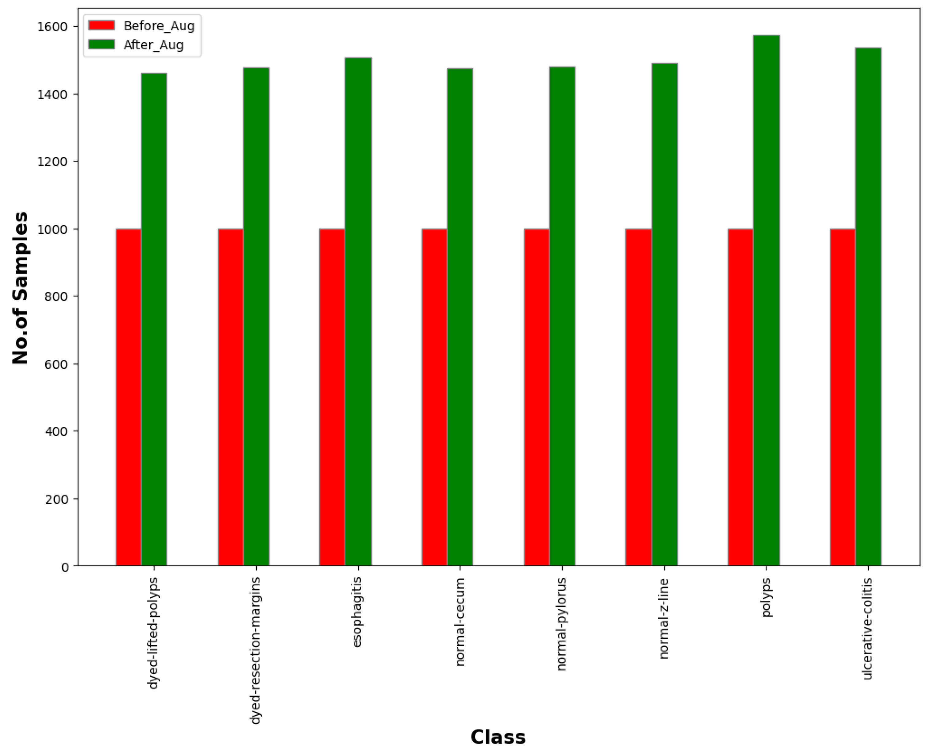
| No. of Samples after Augmentation | 12,000 |
| Training Dataset | 9600 |
| Testing Dataset | 2400 |
| Ensemble Model | Accuracy |
|---|---|
| ResNet50 + InceptionV3 | 90.32 |
| InceptionV3 + DenseNet201 | 87.00 |
| ResNet50 + DenseNet201 | 89.43 |
| DenseNet201 + InceptionV3 + ResNet201 | 95.00 |
| Options | DenseNet201 | InceptionV3 | ResNet50 | Average Ensemble | Weighted Average Ensemble |
|---|---|---|---|---|---|
| Optimizer | Adam | Adam | Adam | Adam | Adam |
| Batch Size | 32 | 32 | 32 | 32 | 32 |
| Epochs | 50 | 50 | 50 | 50 | 50 |
| Learning Rate | 0.0001 | 0.0001 | 0.0001 | 0.0001 | 0.0001 |
| Training Time | 39 m 76 s | 17 m 41 s | 14 m 34 s | 68 m 73 s | 69 m 95 s |
| Trainable Parameters | 19,223,880 | 22,978,472 | 24,739,400 | 66,941,752 | 66,941,752 |
| No. of features extracted | 8 | 8 | 8 | Nil | Nil |
| Model | KVASIR v2 Dataset Accuracy |
|---|---|
| DenseNet201 (M1) | 94.54 |
| InceptionV3(M2) | 88.38 |
| ResNet50 (M3) | 90.58 |
| Model Averaging Ensemble | 92.96 |
| Weighted Average Ensemble | 95.00 |
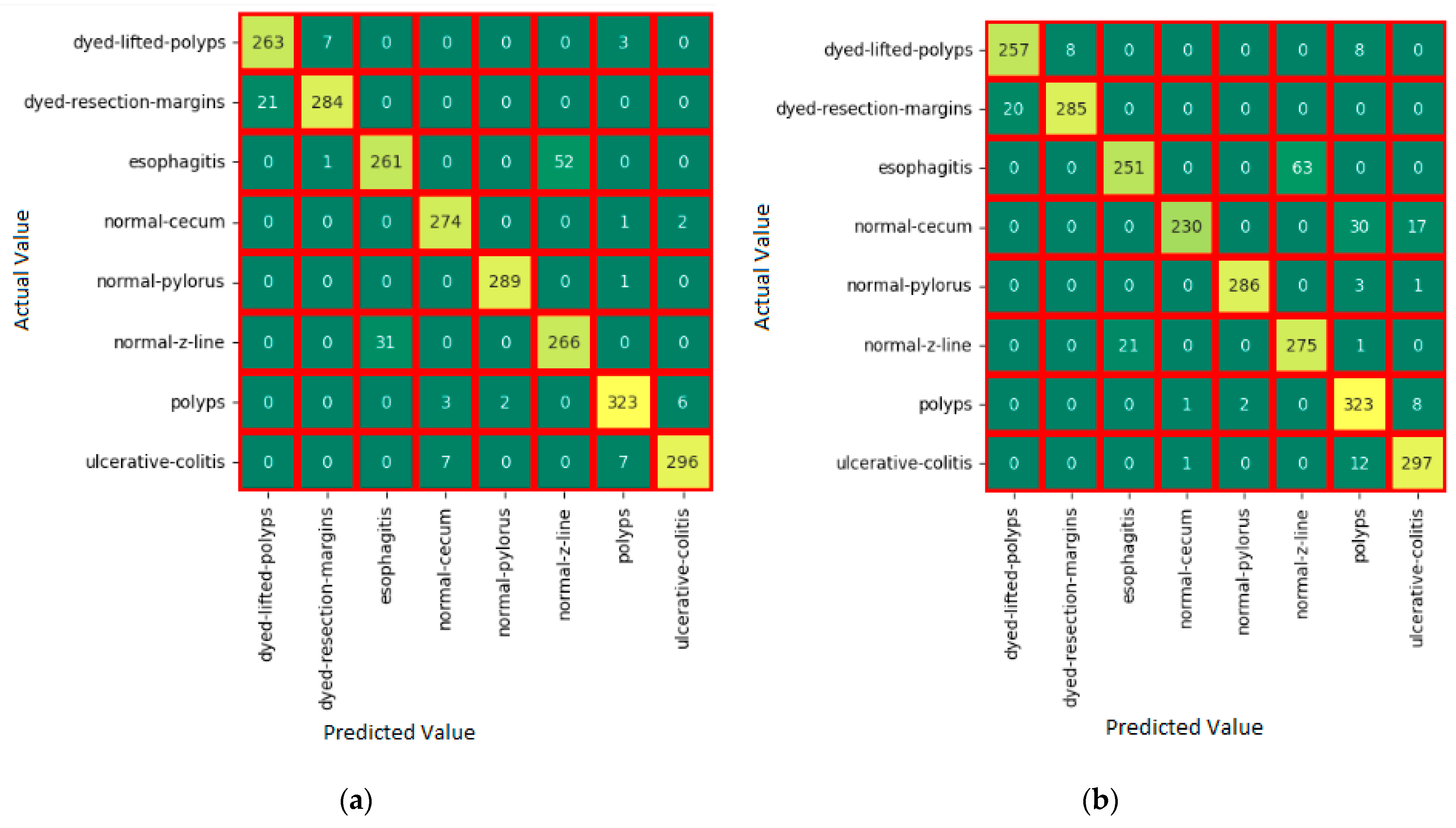
| Class | Precision | Recall | Fl-Score | ||||||
|---|---|---|---|---|---|---|---|---|---|
| Ml | M2 | M3 | Ml | M2 | M3 | Ml | M2 | M3 | |
| dyed-lifted-polyps | 95.70 | 92.00 | 97.52 | 95.67 | 92.60 | 78.70 | 95.19 | 92.72 | 87.27 |
| dyed-resection-margins | 96.01 | 96.86 | 84.76 | 95.75 | 93.15 | 98.36 | 96.38 | 95.45 | 90.59 |
| esophagitis | 93.98 | 79.52 | 86.97 | 83.81 | 82.31 | 65.93 | 88.85 | 80.48 | 74.35 |
| Normal-cecum | 97.11 | 96.78 | 94.12 | 99.19 | 90.47 | 91.78 | 98.14 | 93.07 | 92.95 |
| normal-pylorus | 98.32 | 97.26 | 86.29 | 99.31 | 82.59 | 100.00 | 98.79 | 89.92 | 92.12 |
| normal-z-line | 84.42 | 73.70 | 71.96 | 93.85 | 86.69 | 86.60 | 88.60 | 79.42 | 78.86 |
| polyps | 98.22 | 91.16 | 97.98 | 96.51 | 88.72 | 81.22 | 97.37 | 89.37 | 88.58 |
| ulcerative-colitis | 96.32 | 90.19 | 85.64 | 98.87 | 94.55 | 98.94 | 97.57 | 92.85 | 90.79 |
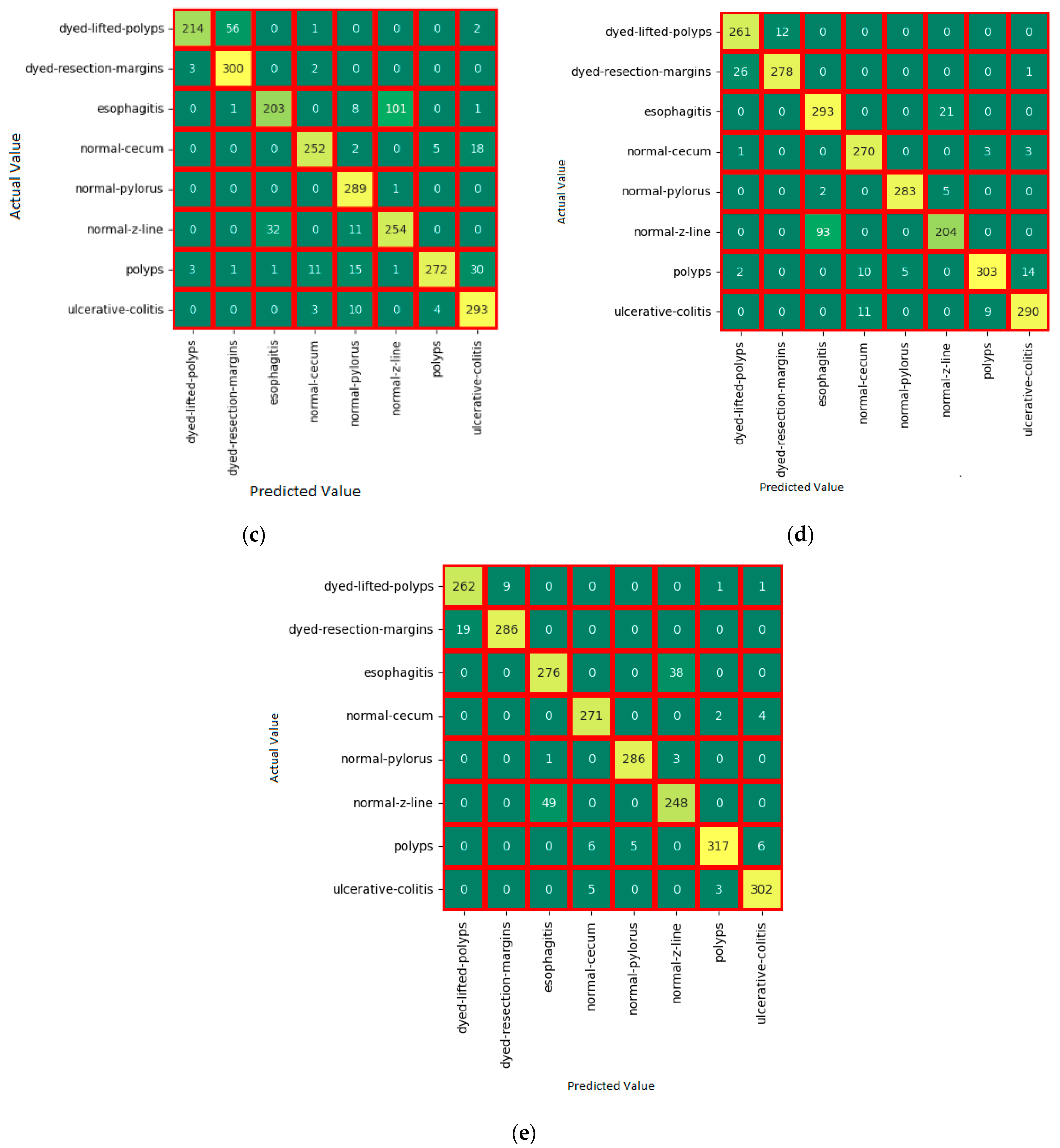
| Class | Precision | Recall | Fl-Score | |||
|---|---|---|---|---|---|---|
| Model Average Ensemble | Weighted Average Ensemble | Model Average Ensemble | Weighted Average Ensemble | Model Average Ensemble | Model Average Ensemble | |
| dyed-lifted-polyps | 93.52 | 93.00 | 94.70 | 96.85 | 93.27 | 94.10 |
| dyed-resection-margins | 97.76 | 97.96 | 93.36 | 93.45 | 95.59 | 95.12 |
| Esophagitis | 92.97 | 89.78 | 80.93 | 83.44 | 86.35 | 86.88 |
| Normal-cecum | 99.12 | 96.45 | 83.78 | 99.88 | 90.95 | 98.65 |
| normal-pylorus | 99.29 | 99.12 | 99.97 | 100.00 | 99.12 | 99.45 |
| normal-z-line | 81.96 | 84.11 | 93.97 | 90.78 | 87.89 | 87.77 |
| Polyps | 86.98 | 96.32 | 97.60 | 97.12 | 91.58 | 97.64 |
| ulcerative-colitis | 92.64 | 97.89 | 96.22 | 95.78 | 94.79 | 96.33 |
| Previous Studies | Model | Accuracy | Dataset Samples | Augmentation |
|---|---|---|---|---|
| Mosleh [1] | AlexNet | 97.00% | 5000 images with 5 classes | Not done |
| GoogleNet | 96.70% | |||
| ResNet50 | 95.00% | |||
| YogaPriya [12] | Transfer Learning | 96.33% | 5000 images | Done |
| Zenebe [13] | CNN based on Spacial attention Mechanism | 93.19% | KVASIR v2 with 8000 images | Done |
| Muhammed [16] | Weighted Avg | 95.00% | KVASIR with 4000 images | Done |
| Afriyie et al. [34] | Dn-CapsNet | 94.16% | KVASIR v2 with 5000 images | Not done |
| Pozdeev et al. [35] | Two Stage Classification | 88.00% | KVASIR v2 with 8000 images | Done |
| Proposed Weighted Average Ensemble | 95.00% | KVASIR v2 with 8000 images | Done | |
Disclaimer/Publisher’s Note: The statements, opinions and data contained in all publications are solely those of the individual author(s) and contributor(s) and not of MDPI and/or the editor(s). MDPI and/or the editor(s) disclaim responsibility for any injury to people or property resulting from any ideas, methods, instructions or products referred to in the content. |
© 2023 by the authors. Licensee MDPI, Basel, Switzerland. This article is an open access article distributed under the terms and conditions of the Creative Commons Attribution (CC BY) license (https://creativecommons.org/licenses/by/4.0/).
Share and Cite
Gunasekaran, H.; Ramalakshmi, K.; Swaminathan, D.K.; J, A.; Mazzara, M. GIT-Net: An Ensemble Deep Learning-Based GI Tract Classification of Endoscopic Images. Bioengineering 2023, 10, 809. https://doi.org/10.3390/bioengineering10070809
Gunasekaran H, Ramalakshmi K, Swaminathan DK, J A, Mazzara M. GIT-Net: An Ensemble Deep Learning-Based GI Tract Classification of Endoscopic Images. Bioengineering. 2023; 10(7):809. https://doi.org/10.3390/bioengineering10070809
Chicago/Turabian StyleGunasekaran, Hemalatha, Krishnamoorthi Ramalakshmi, Deepa Kanmani Swaminathan, Andrew J, and Manuel Mazzara. 2023. "GIT-Net: An Ensemble Deep Learning-Based GI Tract Classification of Endoscopic Images" Bioengineering 10, no. 7: 809. https://doi.org/10.3390/bioengineering10070809