Article

Optimization Design and Performance Analysis of a Bionic Knee Joint Based on the Geared Five-Bar Mechanism

School of Mechanical Engineering, Northwestern Polytechnical University, Xi’an 710072, China
*
Authors to whom correspondence should be addressed.
Bioengineering 2023, 10(5), 582; https://doi.org/10.3390/bioengineering10050582
Submission received: 7 April 2023 / Revised: 5 May 2023 / Accepted: 9 May 2023 / Published: 11 May 2023
(This article belongs to the Special Issue Multiscale Modeling in Computational Biomechanics)

Abstract

:
Animal joint motion is a combination of rotation and translational motion, which brings high stability, high energy utilization, and other advantages. At present, the hinge joint is widely used in the legged robot. The simple motion characteristic of the hinge joint rotating around the fixed axis limits the improvement of the robot’s motion performance. In this paper, by imitating the knee joint of a kangaroo, we propose a new bionic geared five-bar knee joint mechanism to improve the energy utilization rate of the legged robot and reduce the required driving power. Firstly, based on image processing technology, the trajectory curve of the instantaneous center of rotation (ICR) of the kangaroo knee joint was quickly obtained. Then, the bionic knee joint was designed by the single-degree-of-freedom geared five-bar mechanism and the parameters for each part of the mechanism were optimized. Finally, based on the inverted pendulum model and the Newton–Euler recursive method, the dynamics model of the single leg of the robot in the landing stage was established, and the influence of the designed bionic knee joint and hinge joint on the robot’s motion performance was compared and analyzed. The proposed bionic geared five-bar knee joint mechanism can more closely track the given trajectory of the total center of mass motion, has abundant motion characteristics, and can effectively reduce the power demand and energy consumption of the robot knee actuators under the high-speed running and jumping gait.

Graphical Abstract

1. Introduction

Legged robots, such as bipedal and quadrupedal robots, exoskeletons, and intelligent active prostheses, may be used in field exploration [1,2,3], disaster relief [4,5,6,7], home services [8,9,10], and medical rehabilitation [11,12,13,14], and have the potential to change human life in the future. Many researchers have already conducted a lot of research in the field of legged robots, showing astoundingly excellent results, such as Boston Dynamics’ bipedal robot Atlas, which dances like a real person [15], and the quadrupedal robot ANYmal from ETH Zurich, which takes only 31 min to climb a 120 m high mountain (a total distance of 2.2 km), which is 4 min faster than a human on foot [16]. However, the energy efficiency of the various legged robots that are now publicly available is still significantly lower than that of animals with similar locomotion [17,18], and the input power required to complete their locomotion is extremely high, which leads to the problem caused by the large size and weight of the drive system.
Legged robots usually consist of a control module, a drive module, and a motion executive mechanism composed of links. Some researchers have studied intelligent control methods [19,20,21] and high-performance actuators [22,23,24,25] to improve the motion stability and power density of legged robots with excellent results, but they are now gradually encountering development bottlenecks. Other researchers have started from the optimization design of the executive mechanism [17,26,27,28] to solve the above problems.
The hardware structure of legged robots consists mainly of links that are usually connected by revolute joints, but may also be connected by prismatic joints. With the continuous development in the field of biomechanics, numerous studies on the leg joints of mammals, especially the knee and ankle joints [29,30,31,32], have shown that these two joints consist of irregularly shaped bones with the characteristic of multi-axis rotation, that is, their instantaneous center of rotation (ICR) trajectory presents a J-shaped curve. Such joints have greater foot clearance and smaller flexion angles than the uniaxial joints commonly used in legged robots, as well as better ground reaction forces to maintain motion stability. Revolute joints and prismatic joints with simple movement rules have difficulty in imitating the movement characteristics of biological joints, so they cannot obtain the high efficiency and high stability of biological locomotion.
To improve the bionic properties of the joints in legged robots, researchers have proposed various innovative mechanisms to achieve the motion patterns of the biological knee and ankle joints. In the field of robotics, A. Hamon designed the knee joint of a biped robot with the four-bar mechanism [33] and the crossed four-bar mechanism [34], which reduced the energy consumption of the robot and the impact of the foot against the ground during walking. Alexander G mimicked the design of the human knee joint by introducing a single sliding link and replicating the condylar surfaces of the femur and tibia [35]. Yixiang L used planetary gear transmission [36] to achieve changes in the instantaneous center of rotation of the designed knee joint, which outperformed the traditional hinge knee joint in terms of the range of motion and power consumption. However, the design basis of these joint mechanisms, i.e., the ICR curves of the knee and ankle joints of the referenced organisms, were obtained by measuring the parameters of the bone shapes at the biological joints. The period of measurement and processing of experimental data is very long, so it is difficult to realize the fast and automatic design process in the bionic joint design for different bone shapes (such as different bionic objects). At present, the technology for acquiring the surface contour of the target object by image processing technology has a certain foundation, and the application of image processing technology to acquire the surface contour of the target joint is expected to achieve the rapid determination of the optimization target for the design of the bionic joint mechanism and, thus, speed up the design process.
In the field of mechanical exoskeletons and prostheses, Michał O designed a new adjustable knee joint mechanism based on a cross four-bar mechanism [37] by introducing two additional degrees of freedom, which can achieve a variety of knee trajectories. Yonghong Z applied gait acquisition technology to design a six-bar mechanism prosthesis knee joint [38], which can help amputees to accomplish a variety of gait patterns. The main design principle of these joint mechanisms is to make the motion curves of the designed joints fit the actual human knee and ankle motion patterns as much as possible, which facilitates the designed exoskeleton and prosthesis to precisely follow the human lower limb motion. Legged locomotion is mainly divided into walking, running, jumping, and other modes. Humans only have high stability and energy utilization in low-speed walking mode, while in high-speed running, jumping, and other movement modes, cheetahs, kangaroos, and other creatures have obvious advantages, their joints are excellent bionic objects, which may be able to improve the high-speed mobility and energy utilization efficiency of legged robots during running and jumping.
Moreover, current studies mainly discuss the influence of different knee joints on the kinematic performance of bipedal or quadrupedal robots in walking locomotion mode, such as knee extension, foot clearance, and energy consumption [35,36,39,40]. Research on the kinematic performance of mechanical joints based on ICR trajectories of biological joints during high-speed gaits (running and jumping) has not been published, which limits the further application of bionic joints in legged robots.
In the real wild world, kangaroos have the advantages of fast locomotion, robust jumping motion, and low energy consumption compared to other running and jumping quadrupeds. When a kangaroo reaches a certain jumping speed, its oxygen consumption is lower than that of a quadruped with the same mass and speed [41]. During high-speed gaits, such as running and jumping, it has been shown that the knee joint provides the greatest torque and plays a major role in energy consumption [42]. In this paper, by imitating and researching the motion of the kangaroo knee joint, the knee joint mechanism of the legged robot is designed based on the planar multi-bar mechanism, to improve the joint trajectory richness of the legged robot, while reducing the energy cost of the robot actuators during the high-speed gait. The following are the main contributions from the paper:
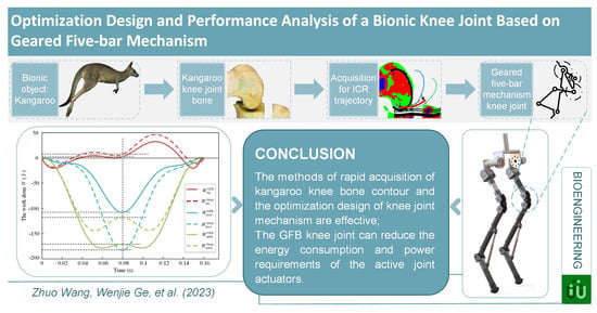
  • Rapid acquisition for the ICR trajectory of the knee joint. Based on the image of the kangaroo leg bone, the contact curve between the kangaroo femur and tibia was automatically acquired using a high-order polynomial fitting method with computer image processing technology;
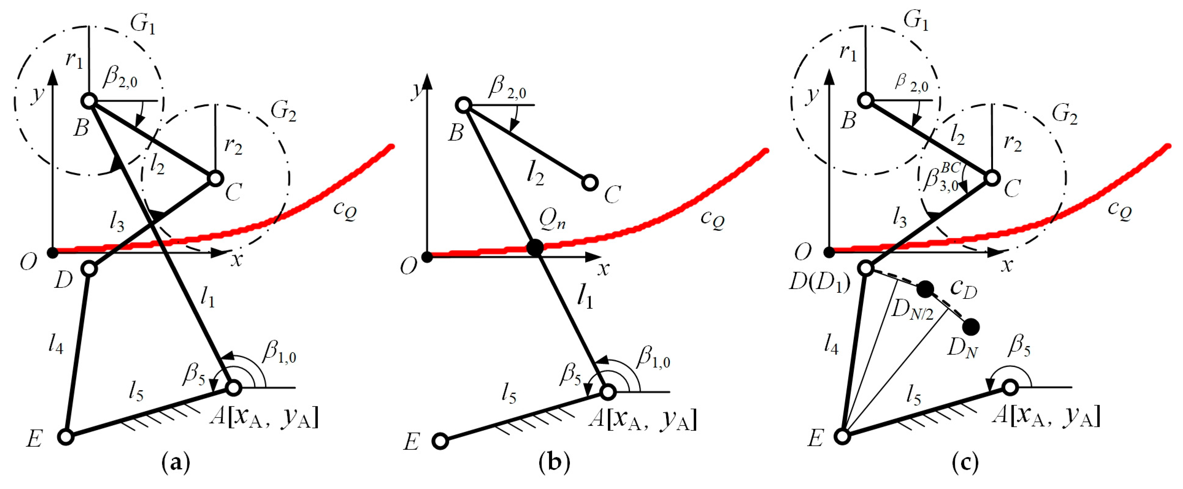
  • Kangaroo-inspired knee joint mechanism design and optimization. The bionic knee joint was designed by a geared five-bar (GFB) mechanism with a single-degree-of-freedom and the parameters for each part of the mechanism were optimized. The ICR trajectory of the kangaroo knee joint was accurately tracked, and the rotation angles of the thigh and tibia in the designed mechanism were consistent with the motion data on the kangaroo lower limb;
  • Performance analysis of the GFB joint during high-speed gaits. Based on the spring inverted pendulum model, the Newton–Euler recursive method was used to establish the dynamics model of the single leg of the robot in the landing stage and the centroid trajectory of the robot model was planned. The effects of the hinge joint mechanism and the GFB joint mechanism on the required driving power and energy consumption of the robot at high speed were compared and analyzed.
The remainder of this paper is organized as follows: In Section 2, we acquire the ICR trajectory of the kangaroo knee joint, and design and optimize the GFB mechanism to accurately track this trajectory; in Section 3, a single-leg model of the robot with the GFB knee joint and hinge knee joint is constructed, and the kinematic performance of these two mechanisms is compared and analyzed; in Section 4, the required driving power and energy of the two knee joints are analyzed; finally, the conclusions and other reflections from the paper are provided in Section 5.

2. The Design and Modeling of a New Bionic Knee Joint Mechanism

2.1. The ICR Analysis of the Knee Joint of the Australian Grey Kangaroo

In this section, the knee joint of an Australian grey kangaroo is studied. Kangaroos are typically jumping animals that can travel long distances at speeds of up to 50 km/h. During a long journey, kangaroo hopping has a low energy consumption [41]. This advantage may be related to the motion characteristics of the kangaroo leg joints. We studied the knee bones of the grey kangaroo to obtain the ICR curve of the femur relative to the tibia. Apparently, the skin, muscles, and bones in the kangaroo’s legs move periodically during jumping, and their movement characteristics are different. Compared with skin and muscles, bones are more similar to rigid bodies, and pictures of leg bones are easy to obtain. Therefore, studying the skeleton picture is a convenient way to obtain the ICR curve.
The skeleton picture (Figure 1a) of the kangaroo knee joint used in this paper is from an adult eastern Australian grey kangaroo (Macropus giganteus), which belongs to the skeletal specimen collection in the Australian Museum [43]. In Figure 1a, the condyles of the femur and tibia of the kangaroo are complete, grayish white, with a clear surface contour, and accurate relative position. In Figure 1a, there is a metal bracket blocking the tibia and the photo must be processed to obtain a clearer image. To make the data obtained after image processing more accurate, we enlarge the original image four times, that is, the scale of Figure 1 and Figure 2 is 4:1. We use the image processing toolbox in MATLAB to process the original photos into RGB images of the knee joint bones (Figure 1b), and use the ginput function to conveniently collect the contact curves of the femur and tibia.
In Figure 1b, the tibial curve can be obtained using a polynomial fitting method for the tibial acquisition points in the Cartesian coordinate system. The tibial curve equation is as follows:
y t = f t ( x t ) = j = 0 4 P j t x t j ,
where P j t is the polynomial coefficient, xt and yt are the x-coordinate value and y-coordinate value of the point on the fitted curve, and x t x m i n , x m a x . Moreover, xmin is the minimum x-coordinate value of the tibial collection point, and xmax is the maximum x-coordinate value of the tibial collection point. The degree of the sum polynomial is 4.
The femoral collection point in Figure 1b cannot fit a polynomial in a Cartesian coordinate system, but it can fit a polynomial in a polar coordinate system. The fitting polynomial of the femoral curve is detailed below.
This is example 1 of an equation:
r f = f f ( θ f ) = k = 0 6 P k f θ f k ,
where P k f is the polynomial coefficient, θf is the polar angle of a point on the curve, and rf is the corresponding polar diameter. The degree of the sum polynomial is 6.
In Figure 1b, the curve of the femur and the curve of the tibia are not in contact. The reason is that in addition to the condyle of the femur and the condyle of the tibia, the knee joint of the kangaroo also contains patella, meniscus, and synovium, etc., which have been removed from the bone specimens. Among them, patella and synovium have almost no influence on the contact surface of the kangaroo knee joint, so they are not considered in the subsequent calculation. The condyle of the femur is covered with a layer of hyaline articular cartilage. The shape of the articular cartilage is consistent with the shape of the articular surface of the bone and the articular cartilage covering the femoral condyle is very thin. Therefore, the external contour curve of the femoral condyle is used as the contact curve of the upper part of the kangaroo knee joint in this paper.
The condyle of the tibia is covered with a cushioning fibrous cartilage called the meniscus. The meniscus thickness is usually more than 3 mm and, therefore, cannot be ignored in subsequent ICR curve calculations. According to the anatomical study of the kangaroo knee joint conducted by the University of Western Australia [44], the contact area between the femoral condyle and meniscus is mainly located in the central area of the meniscus, where the contour curve of the upper surface of the meniscus is basically parallel to that of the tibial condyle. Therefore, this paper introduces a virtual meniscus curve as the lower contact curve of the kangaroo knee joint. This curve can be obtained by translating the tibial curve along the positive y-axis (Figure 2). The polynomial of the meniscus curve is:
y m = f m ( x m ) = f t ( x t ) + b = j = 0 4 P j m x m j ,
where P j m is the polynomial coefficient, xm and ym are the coordinates of the point on the curve c3, and b is the displacement of the curve c3 relative to the curve c2 in the positive direction of the y-axis.
Both the femur curve and tibia curve can be regarded as rigid bodies, and the law of relative motion of the two curves can be regarded as the law of relative motion of the femur and tibia. Before calculating the ICR curve, the movement law of the femur curve relative to the tibia curve must be strictly defined.
In Figure 2a, the rigid body R1 is the femur, and the rigid body R2 is the tibia. The definition of the movement law is as follows: there are moving points PS1, PS2, and fixed points PI, PT1, and PT2 on the curves c1 and c3, respectively. The two moving points can move along their respective curves. The fixed point PI is the starting point of the movement of PS1 and PS2, and the fixed points PT1 and PT2 are the endpoints of the movement of PS1 and PS2, respectively. Moreover, θT1 the polar angle value of the fixed point PT1 is greater than θI the polar angle value of the fixed point PI, and x T 1 the x-coordinate value of PT2 is greater than x I the x-coordinate value of PI. The displacement of points PS1 and PS2 at time t can be expressed as S 2 = f S , 2 ( t ) , where t 0 , t E , and tE is the end time of the movement. At any time t during the full-period motion, the rigid body R2 is fixed to the fixed reference system, and PS1 on the rigid body R1 coincides with PS2 on R2. There is no overlap between R1 and R2, and curve c1 on R1 is tangent to curve c3 on R2.
In Figure 2b, c1 is the femoral curve, c2 is the tibial curve, and c3 is the meniscus curve. The blue curve and green curve with the same shape as curve c1 but in different positions are denoted as c1,n and c1,n+1, respectively. They are different states of the femur curve during the movement of the kangaroo knee joint. Similar to Figure 2a, PS1,n and PS2,n are the moving points on curve c1,n and curve c3, respectively, and PI,n and PT1,n represent the starting point and ending point of the moving point PS1,n on curve c1,n. The definition for each point on the curve c1,n+1 is similar to that of the curves c1 and c1,n, except that the subscript of each point is n + 1. The red curve is the calculated ICR curve and Qn is the discrete point on the curve.
According to the above description, the displacement functions fS1 and fS2 of the points PS1 and PS2 can be used to determine the unique pose of the rigid body R1 relative to the absolute reference frame at time t, that is to say, the rolling and sliding of the rigid body R1 relative to the rigid body R2 can be converted into the movement of points PS1 and PS2 along the curves c1 and c3.
If the motion laws of points PS1 and PS2 on curves c1 and c3 are the same, according to the above definition, the pose of the rigid body R1 at any time can be obtained. The discrete ICR point Qn of the femur relative to the tibia can be calculated according to the vertical bisectors of the points PI,n, PI,n+1, PT1,n, and PT1,n+1 in two adjacent frames, where n is the number of frames. The ICR curve cQ is the connection of all the discrete ICR points.

2.2. The Design and Optimization of the Bionic GFB Knee Joint Mechanism

As shown in Figure 3a, the plane GFB mechanism consists of five connecting bars AB, BC, CD, DE, and AE, and two gears G1 and G2. The bar AE is fixedly connected to the tibial rigid body R2 and fixedly connected to the coordinate system Oxy. The bar BC is fixedly connected to the femur rigid body R1. The origin of the coordinate system Oxy is at point Q1 of the ICR curve cQ. Moreover, xA and yA are the absolute coordinate values of point A. Angle β 1,0 is the initial angle of bar AB and the angle β 2,0 is the initial angle of bar BC. In addition, β 5 is the angle of the fixed bar AE. Furthermore, r1 is the index circle radius of gear G1, r2 is the index circle radius of gear G2, and the transmission ratio of the two gears is λ = r 1 / r 2 .
For the GFB mechanism to simulate the kinematic characteristics of the kangaroo knee joint, not only must the ICR point of the bar BC relative to the bar AE be on the curve cQ at any time, but also the rotation angle of the bar BC must be the same as the kangaroo’s femur. Obviously, this is a multi-variable and multi-objective optimization problem. Using the Kennedy–Aronhold theorem can effectively reduce the number of variables and the objectives in the optimization problem of GFB mechanisms. We split the GFB mechanism shown in Figure 3a into a planar open-chain three-bar mechanism and a planar open-chain four-bar mechanism, thus transforming the optimization problem into two single-objective optimization problems for analysis.
As shown in Figure 3b, the open chain three-bar mechanism is composed of bars AE, AB, and BC. At any number of frames n, the bar AB or its extension line must pass through the point Qn, and the rotation angle of the bar BC is not related to [l2, l5, β2,0, β5]. The process for determining the configuration parameters [xA, yA, l1] of the mechanism is a three variable single-objective optimization problem. According to the Kennedy–Aronhold theorem, the optimization objective function is:
F = min ( f ( x A , y A , l 1 ) ) = min ( n = 1 N ( Δ ϕ B C , n ( x A , y A , l 1 , n ) ( ϕ R 1 , n ϕ R 1 , n 1 ) ) 2 N ) ,
where B C , n is the angle the bar BC has turned, and it is also a function of [xA, yA, l1, n]. Moreover, R 1 , n and R 1 , n 1 are the angles the rigid body R1 has turned at frame n and n−1. N is the total amount of frames. To avoid the bar length being too large or too small, the boundary condition of the bar length l1 is specified as:
30   m m < l 1 < 300   m m ,
According to function (4) and boundary condition (5), the fmincon function is used to find the minimum value of f(xA, yA, l1). The algorithm is the interior-point algorithm, and the tolerance of the variable iteration and the function value are all 10−6. Given a suitable initial value, the objective function converges to the point [40.54, −70.08, 244], where [40.54, −70.08] is the coordinate of point A, and 244 is the bar length l1 of bar AB. The function value at the convergence point is 7.85 × 10⁻⁷.
According to the value of the parameter [xA, yA, l1], the rotation angle changes A B , n and B C , n of bar AB and bar BC can be calculated. Then, the open-chain four-bar mechanism shown in Figure 3c should be analyzed. When the number of frames is n, the rotation angles of bar BC and bar CD relative to the absolute coordinate system are:
ϕ B C , n = β 2 , 0 + i = 1 n Δ ϕ B C , n ϕ C D , n = ϕ B C , n + π + β 3 , 0 B C + i = 1 n Δ ϕ B C , n Δ ϕ A B , n λ ,
where β 3,0 B C is the initial angle of bar CD relative to bar BC. Further, the coordinates of point C and point D are:
x C , n = x A + l 1 cos ( i = 1 n Δ ϕ A B , n ) + l 2 cos ϕ B C , n y C , n = y A + l 1 sin ( i = 1 n Δ ϕ A B , n ) + l 2 sin ϕ B C , n x D , n = x C , n + l 3 cos ϕ C D , n y D , n = y C , n + l 3 sin ϕ C D , n ,
When the GFB mechanism moves from the frame number n = 1 to n = N, the discrete positions of the hinge point D will form a curve cD. Point E is a fixed point relative to the absolute coordinate system, and the bar length l4 of bar DE is constant. Therefore, if the curve cD is a circular arc with point E as the center, the GFB mechanism can simulate the ICR curve and the rotation angle law of the kangaroo knee joint. The objective function of the second optimization of the mechanical structure is:
F = min ( f ( l 2 , l 3 , β 2 , 0 , β 3 , 0 B C ) )   = min ( n = 1 N ( ( x D , n x E ) 2 + ( y D , n y E ) 2 n = 1 N ( x D , n x E ) 2 + ( y D , n y E ) 2 N ) 2 N ) ,
To ensure that the angle values are all within the range of [0, 2π), the boundary conditions of β2,0 and β 3,0 B C are:
[ β 2 , 0 , β 3 , 0 B C ] T [ [ 0 , 0 ] T , [ 2 π , 2 π ] T ) ,
In addition, the length of each bar should not be too large or too small, so the boundary conditions of the bar length are given as follows:
[ l 2 , l 3 ] T [ [ 30 , 30 ] T , [ 300 , 300 ] T ] ,   [ ( x D , n x E ) 2 + ( y D , n y E ) 2 ( x A x E ) 2 + ( y A y E ) 2 ] [ [ 30 , 300 ] [ 30 , 300 ] ] ,
We have calculated the convergence value of the objective function when λ takes different values, and the optimization effect is best if λ = 2. When each parameter takes the value shown in Table 1, the objective function (3) converges, and the function value at the convergence point is 1.36 × 10⁻⁷.
The solid black line in Figure 4a shows the initial configuration of the GFB mechanism and the dashed lines in other colors show the different states. The red solid line is the actual ICR curve of the kangaroo knee joint referenced in the paper and the yellow dashed line is the trajectory of the ICR curve achieved by the designed GFB mechanism. As shown in the figure, these two curves have the same change trend and basically coincide. In Figure 4b, we fix the tibia of the kangaroo, and the rotation angles of the femur during motion is ΦR1,n, i.e., the green solid line. The whole moving process is divided into 1000 equal parts, corresponding to the horizontal coordinates in Figure 4b. In the GFB mechanism, bar AE corresponds to the tibia of the kangaroo and bar BC corresponds to the femur of the kangaroo. The orange dashed line represents the rotation angle of the bar BC. The maximum angle difference between these two curves occurs at the position corresponding to the value 101 of the transverse coordinate, which is 0.0062 rad. The GFB mechanism fits the ICR curve and rotation angle law of the kangaroo knee joint well, which proves the accuracy of the kangaroo knee joint ICR curve acquisition technology and the bionic knee joint mechanism design method proposed in this paper.

3. The Analysis and Discussion of the Inverse Kinematics

It is difficult to explain the influence of the proposed GFB mechanism on the motion performance and driving demand of the legged robot by analyzing the GFB knee joint alone. Therefore, it is necessary to establish a general robot model for comparative analysis. At present, hinge joints are the mainstream design scheme for legged robot knee joints, such as Boston Dynamics’ bipedal robot Atlas [15] and IIT’s bipedal robot WALK-MAN [45], and ETH’s quadrupedal robot ANYmal [1], etc., all of which adopt hinge knee joints. The bipedal robot Cassia [46] and the quadrupedal robot Cheetah [47] from the MIT, transfer their driving motors to the hip using a parallelogram mechanism at the knee joint, which is essentially a hinged knee joint. To explain the influence of the GFB mechanism on the motion performance of the legged robot, we constructed two simplified models of the robot leg with a GFB knee joint and a hinge knee joint. Then, the kinematic performance of these two mechanisms is compared and analyzed. We found that when the size and quality parameters of the main components are similar, there is almost no difference in the total center of gravity (TCM) working space of the two robot mechanisms through forward kinematics analysis. Therefore, the following sections focus on the analysis of the inverse kinematics characteristics of the two mechanisms.

3.1. The Modeling of the Single Leg for Robots

According to the optimization results of the GFB mechanism in Section 2, the bars AB and CD have a positive transmission ratio (Figure 3). There should be three gears articulated with bar BC. The schematic model of the robot mechanisms can be established based on the parameter values of each component, given in Table 1, and the measurement data of the length of the kangaroo femur and tibia and the size parameters of the knee joint bone. The three-dimensional model of the designed legged robot is shown in Figure 5a, which mainly contains the body, thigh, knee joint, shank, foot, and other parts. The hip joint at the connection between the thigh and the body, as well as the knee joint at the connection between the thigh and the shank, are actively driven by motors, while the ankle joint at the connection between the shank and foot is passively driven by a spring.
Figure 5b is a single-leg model of the robot with a GFB knee joint mechanism. For clarity, the mechanism of the knee joint is partially enlarged. Point P1 is the contact point between the toe and the ground. Points P2 to P8 are the hinges between the components. G1, G2, and G3 are the gears. Moreover, G1 and G2 are fixedly connected with bar P7P8 and bar P3P4, respectively. Gear G3 and bar P4P8 are hinged at point P9. Points Cm,1 to Cm,7 are the center points of mass (CM) of the components, and CM Cm,1 and hinge P5 are coincident. Bar P2P3 and bar P3P6 are fixedly connected, and bar P4P5 and bar P4P8 are fixedly connected. The length between the hinge points on each member is represented by l, for example, l12 is the length from points P1 to P2. Point P1 is the intersection of bar P2P3 and the P4P5 extension. Angle θ1 to θ4 is the rotation angle variables of the joint space, and the knee joint angle θ3 is the angle from bar P2P3 to bar P4P5. In addition, θ31 is the angle from bar P2P3 to bar P3P4, and θ32 is the angle from bar P3P4 to bar P4P5. Figure 5c is a single-leg model of the robot with a hinge knee joint mechanism, and the meaning of each symbol is similar to Figure 5b.
In Figure 5b, since the masses of bars P3P4, P6P7, and P7P8 at the knee joint account for a small proportion of the total mass of the robot, it can be considered that there is only one bar P3P4 with mass properties in the knee joint, and the mass of bar P3P4 is the sum of the actual masses of bars P3P4, P6P7, and P7P8. In addition, to facilitate the calculation, a polynomial fitting method is used to establish the relationship between angles θ3, θ31, and θ32, and the polynomial is as follows:
θ 31 = i = 1 4 A i θ 3 i 1 ,   θ 32 = θ 3 θ 31 ,
where A = [−31.35, 0.3927, 4.306 × 10⁻³, −1.968 × 10⁻⁵]. The root mean square (RMSE) of the polynomial is 0.0797 and the coefficient of determination (R-square) is 1.
According to the DH method, the position of the TCM of the model with a GFB mechanism is:
x m 0 = ( m 1 + m 2 + m 3 + m 4 + m 5 ) 1 [ m 1 m 2 m 3 m 4 m 5 ] [ x 1 c m , 1 c 1 y 1 c m , 1 s 1 l 12 c 1 + x 2 c m , 2 c 1 , 2 y 2 c m , 2 s 1 , 2 l 12 c 1 + l 23 c 1 , 2 + x 3 c m , 3 c 1 , 2 , 31 y 3 c m , 3 s 1 , 2 , 31 l 12 c 1 + l 23 c 1 , 2 + l 34 c 1 , 2 , 31 + x 4 c m , 4 c 1 , 2 , 31 , 32 y 4 c m , 4 s 1 , 2 , 31 , 32 l 12 c 1 + l 23 c 1 , 2 + l 34 c 1 , 2 , 31 + l 45 c 1 , 2 , 31 , 32 + x 5 c m , 5 c 1 , 2 , 31 , 32 , 4 y 5 c m , 5 s 1 , 2 , 31 , 32 , 4 ] ,
y 0 m = ( m 1 + m 2 + m 3 + m 4 + m 5 ) 1 [ m 1 m 2 m 3 m 4 m 5 ] [ x 1 c m , 1 s 1 + y 1 c m , 1 c 1 l 12 s 1 + x 2 c m , 2 s 1 , 2 + y 2 c m , 2 c 1 , 2 l 12 s 1 + l 23 s 1 , 2 + x 3 c m , 3 s 1 , 2 , 31 + y 3 c m , 3 c 1 , 2 , 31 l 12 s 1 + l 23 s 1 , 2 + l 34 s 1 , 2 , 31 + x 4 c m , 4 s 1 , 2 , 31 , 32 + y 4 c m , 4 c 1 , 2 , 31 , 32 l 12 s 1 + l 23 s 1 , 2 + l 34 s 1 , 2 , 31 + l 45 s 1 , 2 , 31 , 32 + x 5 c m , 5 s 1 , 2 , 31 , 32 , 4 + y 5 c m , 5 c 1 , 2 , 31 , 32 , 4 ] ,
where s1,2,31 and c1,2,31 are the sine and cosine of the sum of angles θ1, θ2, and θ31, respectively. Other similar symbols indicate similar meanings. The TCM position of the model with a hinge joint mechanism is similar to (13).

3.2. The Analysis of the TCM Trajectory

A large number of studies show that the running and jumping motion can be described by a spring-loaded inverted pendulum (SLIP) model. To carry out the inverse kinematics, it is necessary to plan the trajectory of the centroid and the endpoint of the foot using the SLIP model. Since the knee joint angle of the legged robot in the flight phase is almost unchanged, and the active joints consume little energy in the flight phase, we only analyze the landing phase (the yellow area in Figure 6) of the SLIP model.
As shown in Figure 6, the CM trajectory (the red line) of the symmetric SLIP model is taken as the robot TCM motion trajectory. Where m is the mass of the CM, g is the acceleration of gravity, l is the length from the CM to the toe, and k is the spring stiffness. The direction of the CM horizontal velocity x ˙ a is the positive direction of the x-axis. The model enters the landing phase at position a. The CM reaches its lowest point at position b. The spring is fully extended at position c, and the model takes off. Moreover, ψa is the angle between the CM velocity and the horizontal direction at the beginning of the landing phase, and θ is the angle between the spring axis and the horizontal direction.
During the landing phase, the Euler–Lagrange equation for the CM is:
L = T V = 1 2 m ( l ˙ 2 + l 2 θ ˙ 2 ) m g l sin θ 1 2 k ( l a l ) 2 ,
The equation of motion for the CM is:
{ m l 2 θ ¨ + 2 m l l ˙ θ ˙ m g l cos θ = 0 m l ¨ m l θ ˙ 2 + m g sin θ k ( l a l ) = 0 ,
The state vector of the CM is:
{ p = [ θ θ ˙ l l ˙ ] T p ˙ = [ θ ˙ g cos θ l 2 l ˙ θ ˙ l l ˙ l θ ˙ 2 g sin θ + k m ( l a l ) ] ,
The given parameters and initial values are as follows, m = 20 kg, g = 9.8 m/s2, the free length of the spring is la = 0.850 m, the initial horizontal velocity is x ˙ a = 4.167 m/s, ψa = 135°, and the initial angle between the spring axis and the horizontal direction is θa = 111.8°. The differential Equations (15) are accurately solved with the ode45 function in MATLAB, and the trajectory of the CM is shown in Figure 6.

3.3. Inverse Kinematics Analysis

To facilitate the inverse kinematics analysis of the robot model, (13) is simplified, and the robot TCM position calculation formula is as follows:
x 0 m = a 1 c 1 + a 2 c 1 , 2 + a 3 c 1 , 2 , 31 + a 4 c 1 , 2 , 3 y 0 m = a 1 s 1 + a 2 s 1 , 2 + a 3 s 1 , 2 , 31 + a 4 s 1 , 2 , 3 a 1 = l 12 ( M 0.5 m 1 ) M , a 2 = l 23 ( M m 1 0.5 m 2 ) M a 3 = l 34 ( 0.5 m 3 + m 4 + m 5 ) M , a 4 = m 4 l 45 / 2 + m 5 l 45 M ,
where M is the total mass of the robotic model. Additionally, (17) is further simplified by the trigonometric function formula and the simplified form is:
x 0 m = a 1 c 1 + ( a 2 + a 3 c 31 + a 4 c 3 ) c 1 , 2 ( a 3 s 31 + a 4 s 3 ) s 1 , 2 y 0 m = a 1 s 1 + ( a 2 + a 3 c 31 + a 4 c 3 ) s 1 , 2 + ( a 3 s 31 + a 4 s 3 ) c 1 , 2 A = x 0 m ( a 2 + a 3 c 31 + a 4 c 3 ) + y 0 m ( a 3 s 31 + a 4 s 3 ) B = x 0 m ( a 3 s 31 + a 4 s 3 ) y 0 m ( a 2 + a 3 c 31 + a 4 c 3 ) C = x 0 m 2 + y 0 m 2 + ( a 2 + a 3 c 31 + a 4 c 3 ) 2 + ( a 3 s 31 + a 4 s 3 ) 2 a 1 2 D = a 2 + a 3 c 31 + a 4 c 3 E = a 3 s 31 + a 4 s 3 ,
when the knee angle θ3 and the CM coordinates [0xm, 0ym] are given. Moreover, θ31 can be obtained with (11), and A, B, C, D, and E in (18) can be calculated. The sine and cosine values of θ1, θ1,2, θ31, and θ3 are:
[ c 3 s 3 c 31 s 31 c 1 , 2 s 1 , 2 c 1 s 1 ] = [ c 3 s 3 c 31 s 31 A C ± | B | 4 A 2 C 2 + 4 B 2 2 ( A 2 + B 2 ) 2 A c 1 , 2 C 2 B [ x 0 m D c 1 , 2 + E s 1 , 2 ] / a 1 [ y 0 m D s 1 , 2 E c 1 , 2 ] / a 1 ] ,
The angle values for θ1, θ1,2, θ31, and θ3 can be obtained with the four-quadrant arctangent function atan2. Finally, θ1, θ2, θ31, and θ32 can be obtained according to the relationship between the joint angle, and selected according to:
{ [ θ 1 θ 2 ] T [ 45 120 ] T [ θ 1 θ 2 ] T [ 172 0.5 ] T ,
The solution process for the robot model with the hinge joint, shown in Figure 5c, to track the CM motion trajectory of the SLIP model is similar to the above process.
The solution spaces of the joint angles in the two robot models that track the known TCM trajectories are shown in Figure 7a,b. Obviously, in the region selected by the dotted line of the red ellipse in Figure 7b, the feasible region of the inverse kinematics solution shrinks, which does not appear in Figure 7a. Compared with the hinge knee robot, the GFB knee robot contains more optional angles for each joint when tracking the TCM trajectory shown in Figure 6, which makes it easier to avoid possible collision with the surrounding environment during the landing phase. In other words, the GFB knee robot can run and jump more flexibly. This is an advantage of the GFB knee joint in robot inverse kinematics.

4. The Analysis and Discussion of the Inverse Dynamics

4.1. The Modeling of the Inverse Dynamics

At present, Lagrangian equations are generally used to analyze the inverse dynamics of robots. Compared with the Lagrangian equation, the dynamic analysis using the Newton–Euler recursive method is not only more efficient but can also directly obtain the force of each component in the joint space.
As shown in Figure 8a, since the masses of bars P6P7 and P7P8 are added to bar P3P4, the part of the knee joint framed by the elliptical dotted line is simplified to only one bar P3P4. Moreover, x0, x1, … x5 are the x-coordinate axes of the joint space coordinate system of the robot model, and x0 is the x-axis of the base coordinate system. In addition, xcm,1, x cm,2, … x cm,5 are the x-coordinate axes of the CM space coordinate system. The direction of the z-axis of each coordinate system is outward and the direction of the y-axis is determined according to the right-hand rule. The meanings of the other symbols are the same as in Figure 5b.
The symbol definitions are given as follows: {i} represents the joint space coordinate system, and i is the serial number of each bar, where i = 0, 1, …, 4. In addition, iνi and iωi are the linear and angular velocity of the joint space coordinate system, respectively. Furthermore, iPi+1 is the coordinate vector of the origin of the coordinate system {i + 1} in the coordinate system {i}. Then, θi+1 is the angle between bar i + 1 and bar i.
The angular velocity of the bar i + 1 in the coordinate system {i} is:
ω i i + 1 = ω i i + R i + 1 i θ ˙ i + 1 Z ^ i + 1 i + 1 ,
where R i + 1 i is the rotation matrix from the coordinate system {i} to {i + 1}. The above formula is transformed into the following form with the left multiplied by R i + 1 i :
ω i + 1 i + 1 = R i i + 1 ω i i + θ ˙ i + 1 Z ^ i + 1 i + 1 ,
The linear velocity of bar i + 1 in the coordinate system {i} is:
v i i + 1 = v i i + ω i i × P i i + 1 ,
The transformation is:
v i + 1 i + 1 = R i i + 1 ( v i i + ω i i × P i i + 1 ) ,
Considering that the z-axis of each coordinate system in the two-dimensional plane is always outward, (14) can be transformed into:
ω i + 1 i + 1 = ω i i + θ ˙ i + 1 Z ^ i + 1 i + 1 ,
The first derivative with respect to time t is:
ω ˙ i + 1 i + 1 = ω ˙ i i + θ ¨ i + 1 Z ^ i + 1 i + 1 ,
The tangential linear acceleration of the coordinate system {i + 1} in {i} is:
v ˙ i i + 1 t = ω ˙ i i × P i i + 1 ,
Then, the normal acceleration is:
v ˙ i i + 1 n = ω i i × ( ω i i × P i i + 1 ) ,
The linear acceleration of bar i + 1 in the coordinate system {i} is:
v ˙ i i + 1 = ω ˙ i i × P i i + 1 + ω i i × ( ω i i × P i i + 1 ) + v ˙ i i ,
The transformation with the left multiplied by R i i + 1 is:
v ˙ i + 1 i + 1 = R i i + 1 [ ω ˙ i i × P i i + 1 + ω i i × ( ω i i × P i i + 1 ) + v ˙ i i ] ,
The CM linear acceleration of bar i + 1 in the coordinate system {i + 1} is:
v ˙ i + 1 c m , i + 1 = ω ˙ i + 1 i + 1 × P i + 1 c m , i + 1 + ω i + 1 i + 1 × ( ω i + 1 i + 1 × P i + 1 c m , i + 1 ) + v ˙ i + 1 i + 1 ,
Given the linear acceleration and angular acceleration at the CM of bar i + 1, the Newton–Euler dynamic equation for bar i + 1 is:
F i + 1 i + 1 = m i + 1 v ˙ i + 1 c m , i + 1 N i + 1 i + 1 = I c m , i + 1 i + 1 ω ˙ i + 1 i + 1 + ω i + 1 i + 1 × I c m , i + 1 i + 1 ω i + 1 i + 1 = I c m , i + 1 i + 1 ω ˙ i + 1 i + 1 ,
where i+1Fi+1, i+1Ni+1, and cm,j+1Ii+1 are the force, the torque, and the moment of inertia of bar i + 1 at the CM of itself, respectively, and the value of i+1ωi+1 × cm,i+1Ii+1 i+1ωi+1 in the two-dimensional plane is 0. The formulas (25), (26), …, (32) constitute the extrapolation calculation process for the Newton–Euler recursive method.

4.2. Interpolation Process of the Dynamics

For an open-chain robot, a single bar has the following dynamic balance of force and torque in the CM space:
F i i = f i i R i + 1 i f i + 1 i + 1 N i i = n i i n i i + 1 + ( P i c m , i ) × f i i ( P i i + 1 P i c m , i ) × f i i + 1 ,
where ini and ini+1 are the joint torque of bar i in the coordinate system {i + 1} and {i}, respectively, ifi and ifi+1 are the joint force of bar i in the coordinate system {i + 1} and {i}, respectively, and iPcm,i is the coordinate vector of the CM in the coordinate system {i + 1}. If ifi+1 and ini+1 are left multiplied by the rotation matrix R i + 1 i , the transformation of iNi is:
N i i = n i i R i + 1 i n i + 1 i + 1 P i c m , i × f i i P i i + 1 × R i + 1 i f i + 1 i + 1 + P i c m , i × R i + 1 i f i + 1 i + 1 = n i i R i + 1 i n i + 1 i + 1 P i c m , i × F i i P i i + 1 × R i + 1 i f i + 1 i + 1 ,
The force and torque dynamic balance of the bar in the joint space are:
f i i = R i + 1 i f i + 1 i + 1 + F i i n i i = N i i + R i + 1 i n i + 1 i + 1 + P i c m , i × F i i + P i i + 1 × R i + 1 i f i + 1 i + 1 ,
The torque of bar I at joint i is:
τ i = n i i T Z ^ i i ,
Different from the interpolation process of the robotic arm, there is only force between the toe of the legged robot and the ground, but no torque. Therefore, the interpolation process of the robotic arm dynamics cannot be directly applied. It is worth noting that the recurrence formula for the extrapolation process does not include the force and the motion at the joints, and the interpolation process does not include the angular velocity, the angular acceleration, and the linear acceleration. Without considering the rotation matrices R i + 1 i and R i i + 1 , the Newton–Euler extrapolation process and the interpolation process are independent of each other. Therefore, considering that the structure, the motion, and the force characteristics of the robotics are different, the coordinate system definitions for the extrapolation method and the interpolation method can be different when performing recursive operations.
Fixing the base coordinate system at the joint of the femur bar, the fixed coordinate system of each bar is redefined as shown in Figure 8b, and φ1, φ2, … φ5 are the redefined joint angles. Each CM coordinate system is rotated 180° around the z-axis. Moreover, R i + 1 i , R i i + 1 , iFi, and iNi are written in the new form in the redefined coordinate system, and i = 4, 3, …, 1. Then, (35) and (36) can be used to calculate the joint space force and torque of each bar.

4.3. The Required Drive Torque of the Knee Joint

Section 4.1 and Section 4.2 in this paper have given the calculation methods for the force and torque of each main bar of the GFB joint robot, but the GFB knee joint also contains two bars P6P7 and P7P8 that do not count the mass.
As shown in Figure 9, φ3, φ6, and φ7 are the joint angles, and l3, l6, and l7 are the length of each bar.
The torque at joint P3 of the bar P2P3 is not generated by a physical actuator, but instead is supplied by the force transmitted from the real actuator at joint P4 to bars P6P7 and P7P8. According to the Newton–Euler static equation, the additional torque that the actuator at joint P4 needs to provide is:
τ 3 = τ 3 l 7 s 7 φ λ 23 λ 31 l 3 s 6 φ ,
where λ23 and λ31 are all the gear ratios. The total torque provided at joint P4 is:
τ 2 T o t a l = τ 2 + τ 3 = τ 2 + 2 τ 3 l 7 s 7 φ l 3 s 6 φ ,

4.4. The Analysis of the Energy Cost and Power Requirement

In Figure 7, two sets of joint angle change trajectories belonging to the GFB joint robot and the hinge joint robot are selected as the inverse dynamic calculation variables. The knee joint angle trajectories for these two groups of angle trajectories are the same. By inputting variables into (25), (26), …, (38), we can obtain the inverse dynamics of the GFB joint robot and the hinge joint robot. If the drive torque at the initial moment of the robotic landing phase does work as Wi,0 = 0, the values of work for each joint actuator are:
τ 2 T o t a l = τ 2 + τ 3 = τ 2 + 2 τ 3 l 7 s 7 φ l 3 s 6 φ ,
The driving power of each joint is:
τ 2 T o t a l = τ 2 + τ 3 = τ 2 + 2 τ 3 l 7 s 7 φ l 3 s 6 φ ,
As shown in Figure 6 and Figure 10, the TCMs of the two robots are located at the lowest point at 0.08 s, when the landing phase is symmetrically divided into two parts. At this moment, the total kinetic energy and potential energy of the robot reach the valley value, the elastic potential energy stored in the spring reaches the peak value, and the work conducted by each joint is representative. For the GFB joint model, the hip joint drive work is W h i p G F B = 2.7 J, the knee joint drive work is W k n e e G F B = −108.5 J, and the ankle joint drive work is W a n k l e G F B = −172.6 J. For the hinge joint model, the hip joint drive work is W h i p h i n g e = 7.7 J, the knee joint drive work is W k n e e h i n g e = −184.3 J, and the ankle joint drive work is W a n k l e h i n g e = −118.6 J. The hip and knee joints are driven by active actuators, and the ankle joints are driven by springs. The energy input requirement for the active actuator at the lowest TCM point can be obtained by adding the work of the hip and knee joints. The energy input requirement for the GFB model to the active actuator is 59.91% of the hinge joint model. It can be considered that the GFB knee joint mechanism can transfer the energy cost from the active actuator to the ankle joint elastic passive actuator, and the maximum transmission ratio is about 40.09%.
Figure 11 shows the power demand curves for the two robot models during the landing phase. The maximum absolute values for the active actuator power cost of the GFB joint model and the hinge joint model are 5.104 kW and 5.766 kW, respectively, and the ratio is 88.52%. The ranges of active actuator power cost for the two models are 9.446 kW and 10.83 kW, and the ratio of the GFB model to the hinge model is 87.22%. Furthermore, the standard deviation for the active actuator power cost is:
σ = j = 1 n ( W ˙ T o t a l j j = 1 n W ˙ T o t a l j n ) 2 n ,
where j is the serial number of the frames of motion, and n is the total number of frames. The standard deviation for the active actuator power cost of the GFB model is 2.279 kW, the standard deviation for the active actuator power cost of the hinge model is 3.435 kW, and the ratio is 66.35%. Therefore, the GFB mechanism can effectively reduce the active actuator power cost of the legged robot.

5. Conclusions

To improve the bionic performance and motion ability of the legged robot, a kangaroo-inspired knee joint based on the geared five-bar mechanism is proposed. The bionic knee joint designed in this paper can accurately track the ICR trajectory of the kangaroo knee joint, and the rotation angles of the bars representing the thigh and shank in the mechanism are consistent with the movement law of the kangaroo’s lower limb. This verifies the effectiveness of the rapid acquisition of the kangaroo knee bone contour and the optimization design method of the knee joint mechanism in this paper. The TCM trajectory in the landing phase of the robot is planned using the SLIP model, and the influence of the GFB knee joint and the hinge joint on the motion performance of the robot is investigated by applying the Newton–Euler iteration method. Compared with the hinged knee joint, the GFB knee joint has a larger feasible solution space for the joint angle, that is, the legged robot equipped with the GFB knee joint has more alternative postures and configurations during motion. The GFB knee joint described in this paper can effectively reduce the energy consumption and power required in legged robots. The compact GFB joint can also be applied to other legged motion systems with multiple joints, such as prostheses, exoskeletons, industrial manipulators, etc., which are expected to improve their dynamic performance and reduce power consumption.
The single leg of the robot studied in this paper is not only a legged robot, but also an independent motion module in a multi-legged robot. Therefore, the GFB knee joint mechanism with richer motion trajectories and lower energy consumption can also be applied to the leg mechanism of a multi-legged robot. In addition, the mechanism model shown in Figure 5b can be regarded as a manipulator arm with a fixed base, the bar P1P2 is regarded as the base, the joint P2 is regarded as the base joint, the circle dotted area is regarded as the elbow joint, and joint P5 is regarded as a wrist joint. In this way, the GFB elbow joint mechanism can reduce the power requirements of the wrist and elbow joints on the drive and transfer the energy consumption of the wrist and elbow joint drive to the base joint drive.

Author Contributions

Conceptualization, Z.W. and B.L. (Bo Liu); methodology, Z.W.; software, B.L. (Bin Liu); validation, Z.W., B.L. (Bo Liu) and W.G.; formal analysis, Y.L.; investigation, Y.Z.; resources, W.G.; data curation, S.J.; writing—original draft preparation, Z.W.; writing—review and editing, W.G.; visualization, Y.L.; supervision, Y.Z.; project administration, W.G.; funding acquisition, W.G. All authors have read and agreed to the published version of the manuscript.

Funding

This research was funded by the National Natural Science Foundation of China (50975230).

Institutional Review Board Statement

Not applicable.

Informed Consent Statement

Not applicable.

Data Availability Statement

Not applicable.

Conflicts of Interest

The authors declare no conflict of interest.

References

  1. Hutter, M.; Gehring, C.; Jud, D.; Lauber, A.; Bellicoso, C.D.; Tsounis, V.; Hwangbo, J.; Bodie, K.; Fankhauser, P.; Bloesch, M.; et al. ANYmal—A Highly Mobile and Dynamic Quadrupedal Robot. In Proceedings of the 2016 IEEE/RSJ International Conference on Intelligent Robots and Systems (IROS), Daejeon, Republic of Korea, 9–14 October 2016; pp. 38–44. [Google Scholar] [CrossRef]
  2. Hutter, M.; Diethelm, R.; Bachmann, S.; Fankhauser, P.; Gehring, C.; Tsounis, V.; Lauber, A.; Guenther, F.; Bjelonic, M.; Isler, L.; et al. Towards a Generic Solution for Inspection of Industrial Sites. In Field and Service Robotics; Springer Proceedings in Advanced Robotics; Springer International Publishing: Cham, Switzerland, 2018; Volume 5, pp. 575–589. [Google Scholar] [CrossRef]
  3. Bellicoso, C.D.; Bjelonic, M.; Wellhausen, L.; Holtmann, K.; Günther, F.; Tranzatto, M.; Fankhauser, P.; Hutter, M. Advances in Real-World Applications for Legged Robots. J. Field Robot. 2018, 35, 1311–1326. [Google Scholar] [CrossRef]
  4. Davids, A. Urban Search and Rescue Robots: From Tragedy to Technology. IEEE Intell. Syst. 2002, 17, 81–83. [Google Scholar] [CrossRef]
  5. Klamt, T.; Schwarz, M.; Lenz, C.; Baccelliere, L.; Buongiorno, D.; Cichon, T.; DiGuardo, A.; Droeschel, D.; Gabardi, M.; Kamedula, M.; et al. Remote Mobile Manipulation with the Centauro Robot: Full-body Telepresence and Autonomous Operator Assistance. J. Field Robot. 2020, 37, 889–919. [Google Scholar] [CrossRef]
  6. Röning, J.; Kauppinen, M.; Pitkänen, V.; Kemppainen, A.; Tikanmäki, A. The Challenge of Preparing Teams for the European Robotics League: Emergency. In IS&T International Symposium on Electronic Imaging Science and Technology; IS&T Digital Library: Burlingame, CA, USA, 2017; pp. 22–30. [Google Scholar] [CrossRef]
  7. Winfield, A.F.T.; Franco, M.P.; Brueggemann, B.; Castro, A.; Limon, M.C.; Ferri, G.; Ferreira, F.; Liu, X.; Petillot, Y.; Roning, J.; et al. EuRathlon 2015: A Multi-Domain Multi-Robot Grand Challenge for Search and Rescue Robots. In Towards Autonomous Robotic Systems; Lecture Notes in Computer Science; Springer International Publishing: Cham, Switzerland, 2016; Volume 9716, pp. 351–363. [Google Scholar] [CrossRef]
  8. Dietrich, A.; Bussmann, K.; Petit, F.; Kotyczka, P.; Ott, C.; Lohmann, B.; Albu-Schäffer, A. Whole-Body Impedance Control of Wheeled Mobile Manipulators: Stability Analysis and Experiments on the Humanoid Robot Rollin’ Justin. Auton. Robot. 2016, 40, 505–517. [Google Scholar] [CrossRef]
  9. Melson, G.F.; Kahn, P.H.; Beck, A.M.; Friedman, B.; Roberts, T.; Garrett, E. Robots as Dogs?: Children’s Interactions with the Robotic Dog AIBO and a Live Australian Shepherd. In CHI ’05 Extended Abstracts on Human Factors in Computing Systems; ACM: Portland, OR, USA, 2005; pp. 1649–1652. [Google Scholar] [CrossRef]
  10. Shigemi, S. ASIMO and Humanoid Robot Research at Honda. In Humanoid Robotics: A Reference; Springer: Dordrecht, The Netherlands, 2019; pp. 55–90. [Google Scholar] [CrossRef]
  11. Louie, D.R.; Eng, J.J. Powered Robotic Exoskeletons in Post-Stroke Rehabilitation of Gait: A Scoping Review. J. NeuroEng. Rehabil. 2016, 13, 53. [Google Scholar] [CrossRef] [PubMed]
  12. Yamamoto, K.; Ishii, M.; Hyodo, K.; Yoshimitsu, T.; Matsuo, T. Development of Power Assisting Suit (Miniaturization of Supply System to Realize Wearable Suit). JSME Int. J. Ser. C 2003, 46, 923–930. [Google Scholar] [CrossRef]
  13. Farris, R.J.; Quintero, H.A.; Goldfarb, M. Preliminary Evaluation of a Powered Lower Limb Orthosis to Aid Walking in Paraplegic Individuals. IEEE Trans. Neural Syst. Rehabil. Eng. 2011, 19, 652–659. [Google Scholar] [CrossRef]
  14. Settembre, N.; Maurice, P.; Paysant, J.; Theurel, J.; Claudon, L.; Kimmoun, A.; Levy, B.; Hani, H.; Chenuel, B.; Ivaldi, S. The Use of Exoskeletons to Help with Prone Positioning in the Intensive Care Unit during COVID-19. Ann. Phys. Rehabil. Med. 2020, 63, 379–382. [Google Scholar] [CrossRef]
  15. Boston Dynamics. Atlas. Available online: https://www.bostondynamics.com/atlas (accessed on 5 April 2023).
  16. Miki, T.; Lee, J.; Hwangbo, J.; Wellhausen, L.; Koltun, V.; Hutter, M. Learning Robust Perceptive Locomotion for Quadrupedal Robots in the Wild. Sci. Robot. 2022, 7, eabk2822. [Google Scholar] [CrossRef]
  17. Badri-Spröwitz, A.; Aghamaleki Sarvestani, A.; Sitti, M.; Daley, M.A. BirdBot Achieves Energy-Efficient Gait with Minimal Control Using Avian-Inspired Leg Clutching. Sci. Robot. 2022, 7, eabg4055. [Google Scholar] [CrossRef]
  18. Seok, S.; Wang, A.; Chuah, M.Y.; Hyun, D.J.; Lee, J.; Otten, D.M.; Lang, J.H.; Kim, S. Design Principles for Energy-Efficient Legged Locomotion and Implementation on the MIT Cheetah Robot. IEEE/ASME Trans. Mechatron. 2015, 20, 1117–1129. [Google Scholar] [CrossRef]
  19. Wang, Z.; Kou, L.; Ke, W.; Chen, Y.; Bai, Y.; Li, Q.; Lu, D. A Spring Compensation Method for a Low-Cost Biped Robot Based on Whole Body Control. Biomimetics 2023, 8, 126. [Google Scholar] [CrossRef]
  20. Polet, D.T.; Bertram, J.E.A. An Inelastic Quadrupedal Model Discovers Four-Beat Walking, Two-Beat Running, and Pseudo-Elastic Actuation as Energetically Optimal. PLoS Comput. Biol. 2019, 15, e1007444. [Google Scholar] [CrossRef]
  21. Goswami, A.; Thuilot, B.; Espiau, B. A Study of the Passive Gait of a Compass-Like Biped Robot: Symmetry and Chaos. Int. J. Robot. Res. 1998, 17, 1282–1301. [Google Scholar] [CrossRef]
  22. Wang, Z.; Liu, S.; Huang, B.; Luo, H.; Min, F. Forced Servoing of a Series Elastic Actuator Based on Link-Side Acceleration Measurement. Actuators 2023, 12, 126. [Google Scholar] [CrossRef]
  23. Katz, B.G. A Low Cost Modular Actuator for Dynamic Robots. Ph.D. Thesis, Massachusetts Institute of Technology, Cambridge, MA, USA, 2018. [Google Scholar]
  24. Farve, N.N. Design of a Low-Mass High-Torque Brushless Motor for Application in Quadruped Robotics. Ph.D. Thesis, Massachusetts Institute of Technology, Cambridge, MA, USA, 2012. [Google Scholar]
  25. Ishida, T.; Takanishi, A. A Robot Actuator Development with High Backdrivability. In Proceedings of the 2006 IEEE Conference on Robotics, Automation and Mechatronics, Bangkok, Thailand, 1–3 June 2006; pp. 1–6. [Google Scholar] [CrossRef]
  26. Park, J.; Kim, K.-S.; Kim, S. Design of a Cat-Inspired Robotic Leg for Fast Running. Adv. Robot. 2014, 28, 1587–1598. [Google Scholar] [CrossRef]
  27. Shin, H.; Ishikawa, T.; Kamioka, T.; Hosoda, K.; Yoshiike, T. Mechanistic Properties of Five-Bar Parallel Mechanism for Leg Structure Based on Spring Loaded Inverted Pendulum. In 2019 IEEE-RAS 19th International Conference on Humanoid Robots (Humanoids), Toronto, ON, Canada, 15–17 October 2019; IEEE: Toronto, ON, Canada, 2019; pp. 320–327. [Google Scholar] [CrossRef]
  28. Kenneally, G.; De, A.; Koditschek, D.E. Design Principles for a Family of Direct-Drive Legged Robots. IEEE Robot. Autom. Lett. 2016, 1, 900–907. [Google Scholar] [CrossRef]
  29. Wiczkowski, E.; Skiba, K. Kinetic analysis of the human knee joint. Biol. Sport 2008, 25, 77–91. [Google Scholar]
  30. Holden, J.P.; Stanhope, S.J. The Effect of Variation in Knee Center Location Estimates on Net Knee Joint Moments. Gait Posture 1998, 7, 1–6. [Google Scholar] [CrossRef]
  31. Gerber, C.; Matter, P. Biomechanical Analysis of the Knee after Rupture of the Anterior Cruciate Ligament and Its Primary Repair. An Instant-Centre Analysis of Function. J. Bone Jt. Surgery. Br. 1983, 65, 391–399. [Google Scholar] [CrossRef]
  32. Nägerl, H.; Dathe, H.; Fiedler, C.; Gowers, L.; Kirsch, S.; Kubein-Meesenburg, D.; Dumont, C.; Wachowski, M.M. The Morphology of the Articular Surfaces of Biological Knee Joints Provides Essential Guidance for the Construction of Functional Knee Endoprostheses. Acta Bioeng. Biomech. 2015, 17, 45–53. [Google Scholar]
  33. Hamon, A.; Aoustin, Y. Study of Different Structures of the Knee Joint for a Planar Bipedal Robot. In 2009 9th IEEE-RAS International Conference on Humanoid Robots, Paris, France, 7–10 December 2009; IEEE: Paris, France, 2009; pp. 113–120. [Google Scholar] [CrossRef]
  34. Aoustin, Y.; Hamon, A. Human like Trajectory Generation for a Biped Robot with a Four-Bar Linkage for the Knees. Robot. Auton. Syst. 2013, 61, 1717–1725. [Google Scholar] [CrossRef]
  35. Steele, A.G.; Hunt, A.; Etoundi, A.C. Development of a Bio-Inspired Knee Joint Mechanism for a Bipedal Robot. In Biomimetic and Biohybrid Systems; Mangan, Lecture Notes in Computer Science; Springer International Publishing: Cham, Switzerland, 2017; Volume 10384. [Google Scholar] [CrossRef]
  36. Liu, Y.; Zang, X.; Li, C.; Heng, S.; Lin, Z.; Zhao, J. Design and Control of a Pneumatic-Driven Biomimetic Knee Joint for Biped Robot. In Proceedings of the 2017 IEEE International Conference on Advanced Intelligent Mechatronics (AIM), Munich, Germany, 3–7 July 2017; pp. 70–75. [Google Scholar] [CrossRef]
  37. Olinski, M.; Gronowicz, A.; Ceccarelli, M. Development and Characterisation of a Controllable Adjustable Knee Joint Mechanism. Mech. Mach. Theory 2021, 155, 104101. [Google Scholar] [CrossRef]
  38. Zhang, Y.; Wang, E.; Wang, M.; Liu, S.; Ge, W. Design and Experimental Research of Knee Joint Prosthesis Based on Gait Acquisition Technology. Biomimetics 2021, 6, 28. [Google Scholar] [CrossRef]
  39. Anand, T.; Sujatha, S. A Method for Performance Comparison of Polycentric Knees and Its Application to the Design of a Knee for Developing Countries. Prosthet. Orthot. Int. 2017, 41, 402–411. [Google Scholar] [CrossRef] [PubMed]
  40. Sudeesh, S.; Sujatha, S.; Shunmugam, M.S. The Effects of Polycentric Knee Design and Alignment on Swing Phase Gait Parameters: A Simulation Approach. J. Prosthet. Orthot. 2021, 33, 266–278. [Google Scholar] [CrossRef]
  41. Dawson, T.J.; Taylor, C.R. Energetic Cost of Locomotion in Kangaroos. Nature 1973, 246, 313–314. [Google Scholar] [CrossRef]
  42. Nisell, R. Mechanics of the Knee: A Study of Joint and Muscle Load with Clinical Applications. Acta Orthop. Scand. 1985, 56 (Suppl. S216), 1–42. [Google Scholar] [CrossRef]
  43. Kangaroo Skeleton, Australian Museum. Available online: https://pbase.com/bmcmorrow/australianmuseum (accessed on 11 February 2023).
  44. He, B.; Wu, J.P.; Xu, J.; Day, R.E.; Kirk, T.B. Microstructural and Compositional Features of the Fibrous and Hyaline Cartilage on the Medial Tibial Plateau Imply a Unique Role for the Hopping Locomotion of Kangaroo. PLoS ONE 2013, 8, e74303. [Google Scholar] [CrossRef]
  45. Negrello, F.; Garabini, M.; Catalano, M.G.; Kryczka, P.; Choi, W.; Caldwell, D.; Bicchi, A.; Tsagarakis, N. WALK-MAN Humanoid Lower Body Design Optimization for Enhanced Physical Performance. In Proceedings of the 2016 IEEE International Conference on Robotics and Automation (ICRA), Stockholm, Sweden, 16–21 May 2016; pp. 1817–1824. [Google Scholar] [CrossRef]
  46. Reher, J.; Ma, W.-L.; Ames, A.D. Dynamic Walking with Compliance on a Cassie Bipedal Robot. In Proceedings of the 2019 18th European Control Conference (ECC), Naples, Italy, 25–28 June 2019; pp. 2589–2595. [Google Scholar] [CrossRef]
  47. Bledt, G.; Powell, M.J.; Katz, B.; Di Carlo, J.; Wensing, P.M.; Kim, S. MIT Cheetah 3: Design and Control of a Robust, Dynamic Quadruped Robot. In Proceedings of the 2018 IEEE/RSJ International Conference on Intelligent Robots and Systems (IROS), Madrid, Spain, 1–5 October 2018; pp. 2245–2252. [Google Scholar] [CrossRef]
Figure 1. (a) Grey kangaroo knee joint bone photo; (b) grey kangaroo knee joint bone RGB image.
Bioengineering 10 00582 g001
Figure 2. (a) The schematic diagram of an equivalent rigid body of knee joint bones; (b) ICR curve analysis.
Bioengineering 10 00582 g002
Figure 3. The optimization process for the GFB mechanism: (a) definition of the coordinate system and key parameters of the GFB mechanism; (b) the open-chain three-bar mechanism to determine the configuration parameters; (c) the open-chain four-bar mechanism to determine the remaining parameters.
Bioengineering 10 00582 g003
Figure 4. (a) The ICR curves of the GFB mechanism and the kangaroo; (b) the rotation angle trajectory of the GFB mechanism and the kangaroo.
Bioengineering 10 00582 g004
Figure 5. The schematic diagrams of the robotic mechanical structure with the GFB knee joint and the hinge knee joint: (a) 3D model of the legged robot; (b) the single-leg model of the robot with a GFB knee joint; (c) the single-leg model of the robot with a hinge knee joint.
Bioengineering 10 00582 g005
Figure 6. The SLIP model.
Bioengineering 10 00582 g006
Figure 7. The solution spaces of the joint angles: (a) the robot with the GFB joint; (b) the robot with the hinge joint.
Bioengineering 10 00582 g007
Figure 8. The coordinate systems and variables definition for the robotic models: (a) the extrapolation process; (b) the interpolation process.
Bioengineering 10 00582 g008
Figure 9. The coordinate systems and variables definition for the GFB mechanism.
Bioengineering 10 00582 g009
Figure 10. The energy consumption of the joint actuators.
Bioengineering 10 00582 g010
Figure 11. The required power of the joint actuators.
Bioengineering 10 00582 g011
Table 1. The parameters of the GFB mechanism when λ = 2.
VariableValueVariableValue
l1 (mm)244.00xA (mm)40.54
l2 (mm)145.90yA (mm)−70.08
l3 (mm)87.20Β1,0 (rad)2.0952
l4 (mm)149.50β2,0 (rad)0.4396
l5 (mm)120.20β5 (rad)−2.8709
Disclaimer/Publisher’s Note: The statements, opinions and data contained in all publications are solely those of the individual author(s) and contributor(s) and not of MDPI and/or the editor(s). MDPI and/or the editor(s) disclaim responsibility for any injury to people or property resulting from any ideas, methods, instructions or products referred to in the content.

