

CNN-Based Identification of Parkinson’s Disease from Continuous Speech in Noisy Environments
 , ,
, ,
Abstract
:1. Introduction
1.1. Related Work—Features Extraction
1.2. Related Work—Classifiers
1.3. Present Study
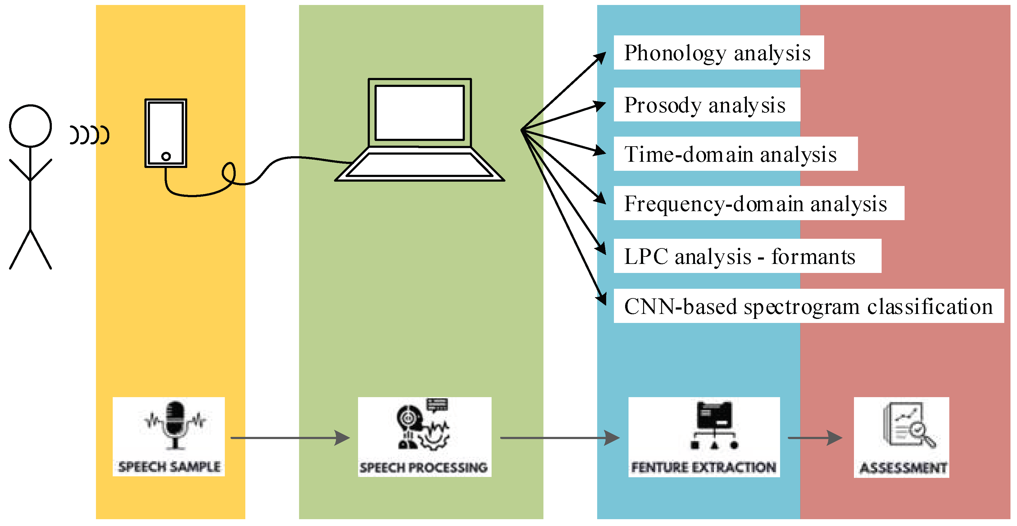
2. Materials and Methods
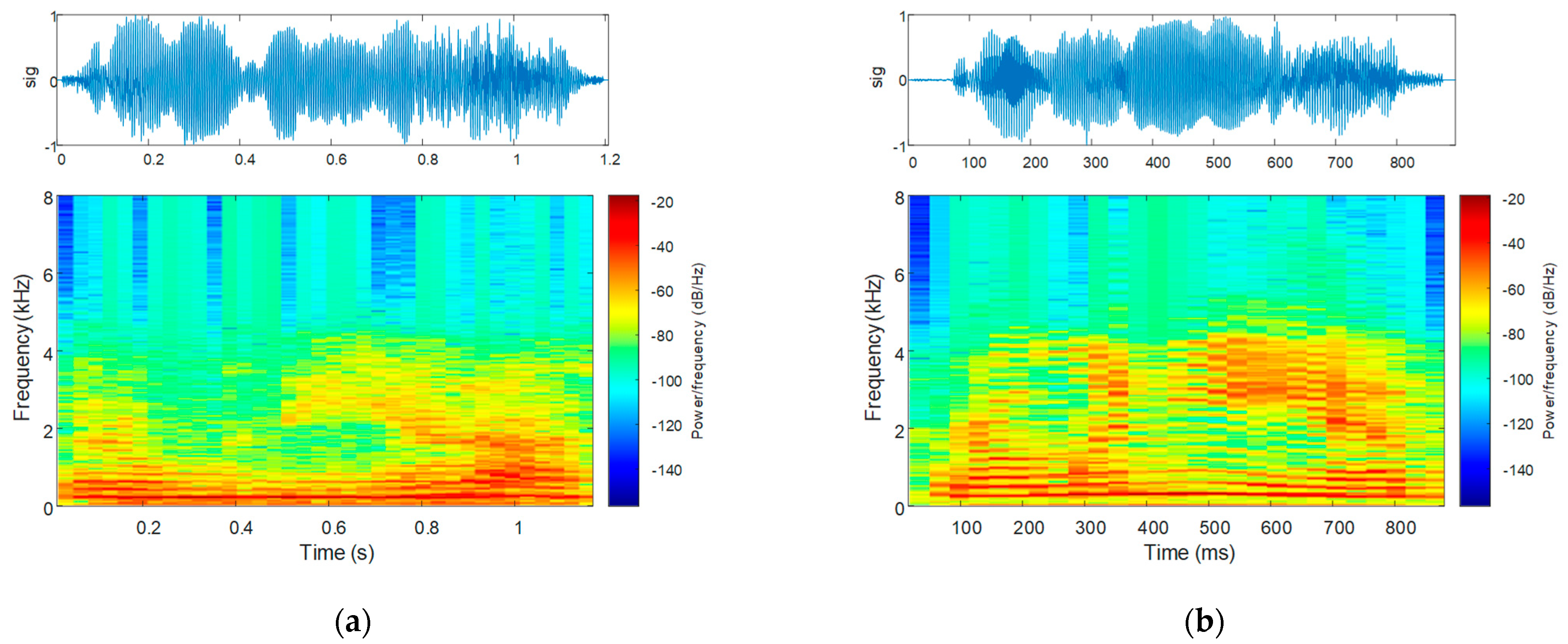
2.1. Speech Acquisition Protocol
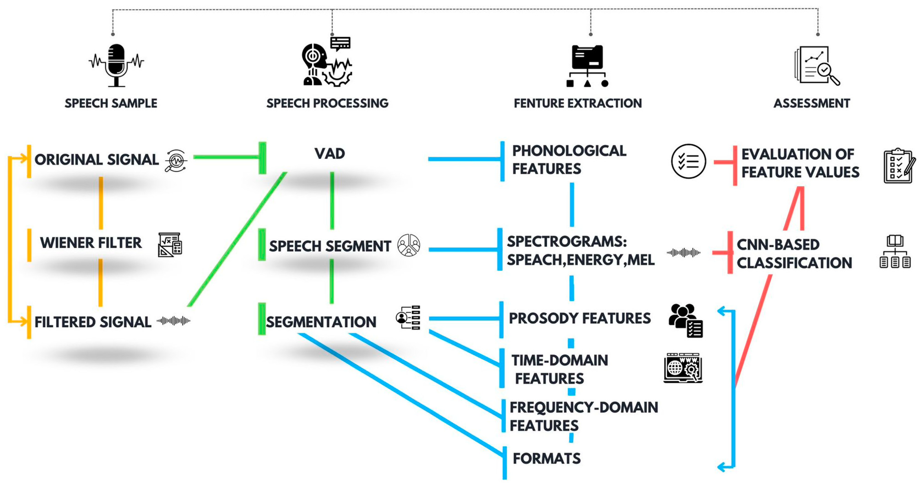
2.2. Proposed Workflow for Speech Processing and Assessment
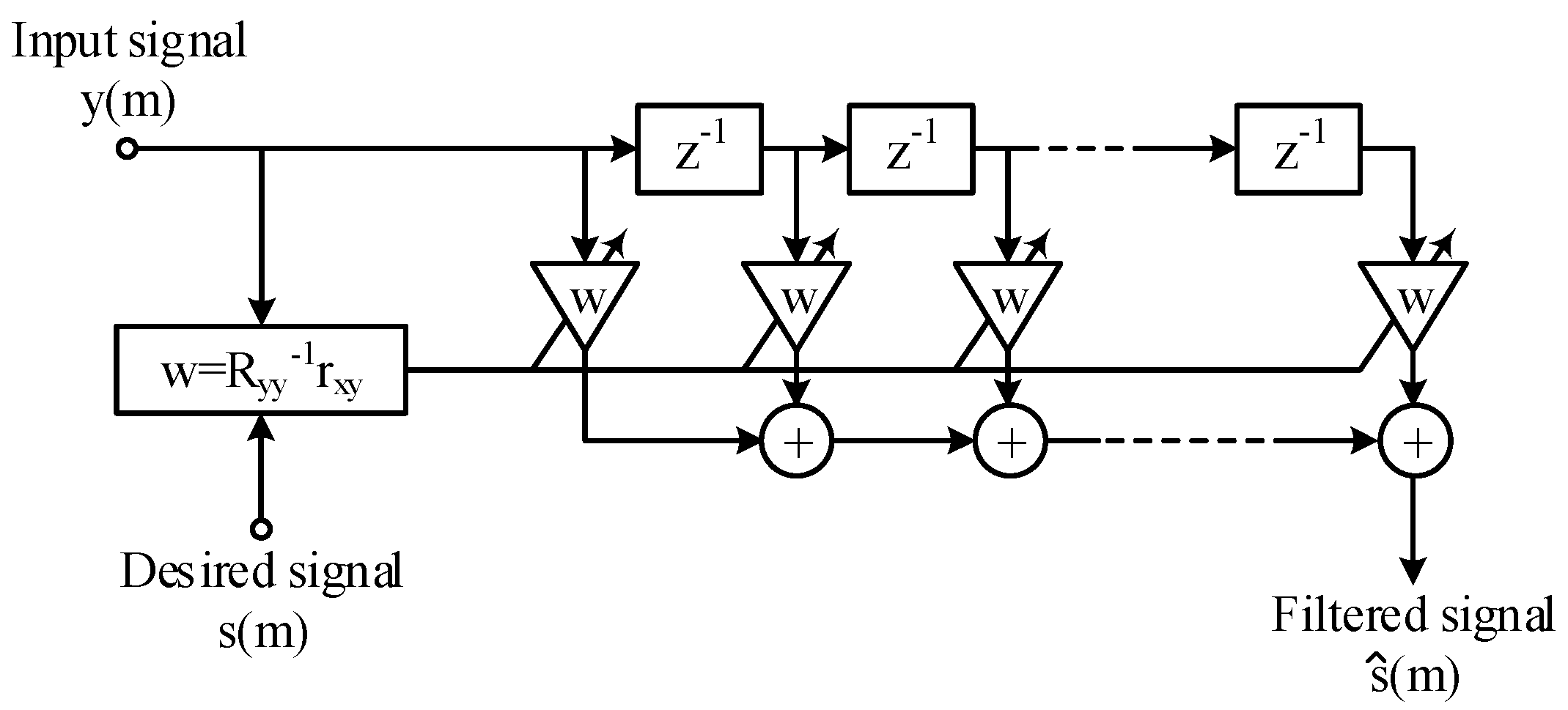
2.2.1. Mathematical Formula of the Wiener Filter
Time-Domain Equations
Frequency-Domain Equations
Wiener Filter Performance Metrics
2.2.2. Feature Extraction for Parkinsonian Speech Assessment
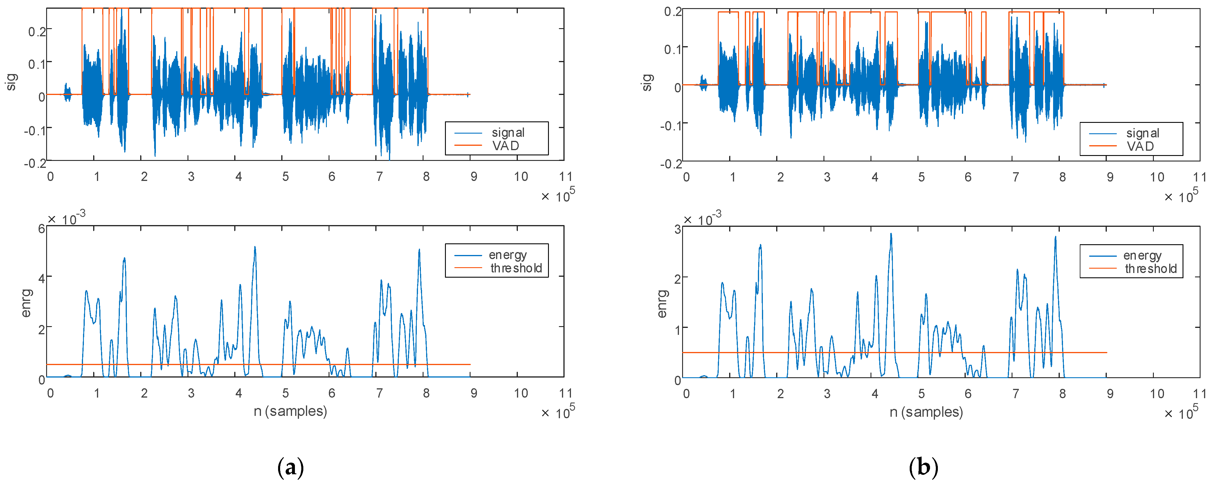
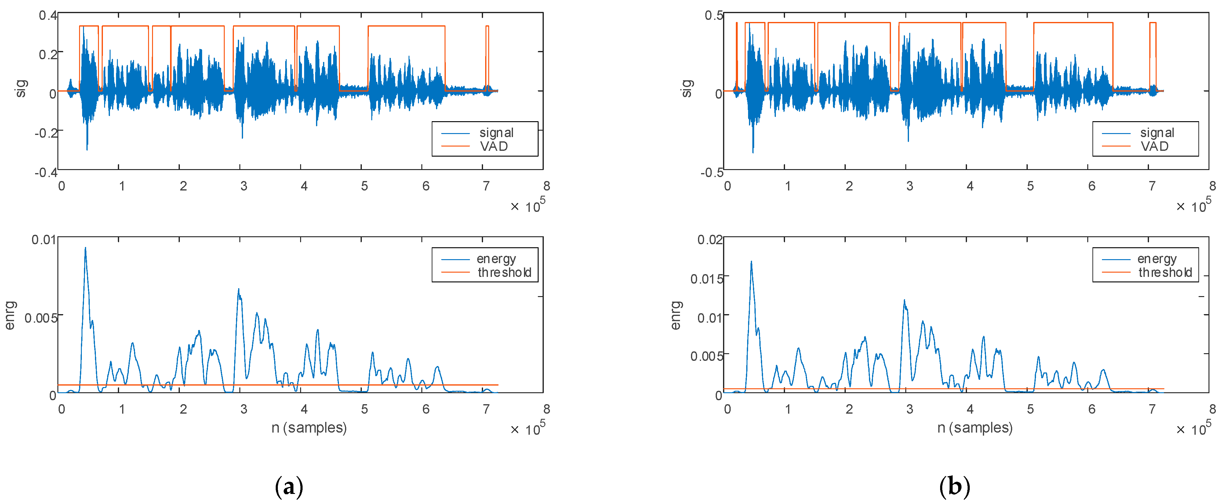
Phonological Analysis
- The uttering count corresponds to the number of detected voice activities,
- The pause count corresponds to the number of detected pauses,
- The speech rate, expressed in words/minute, is determined as the number of utterings expressed throughout the complete speech duration,
- The pause time, expressed in seconds, is determined as the total duration of pause segments (to be noticed is that we have eliminate the initial and final pauses prior to assessment).
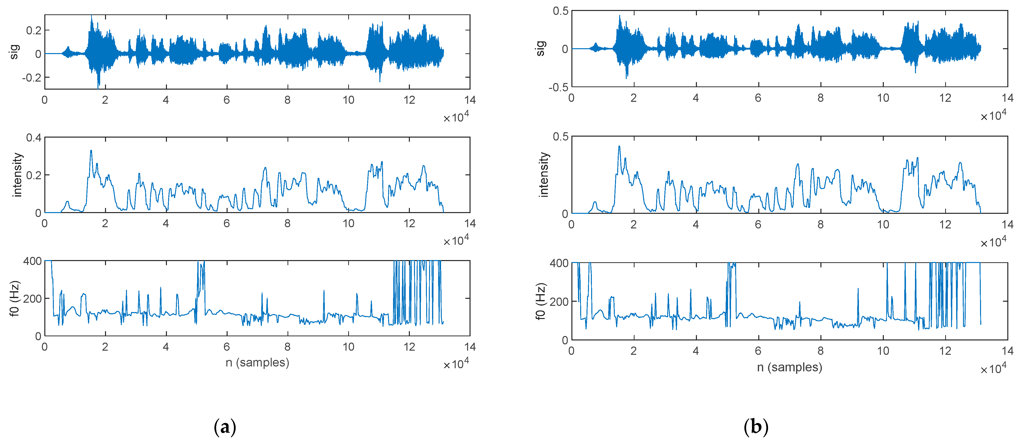
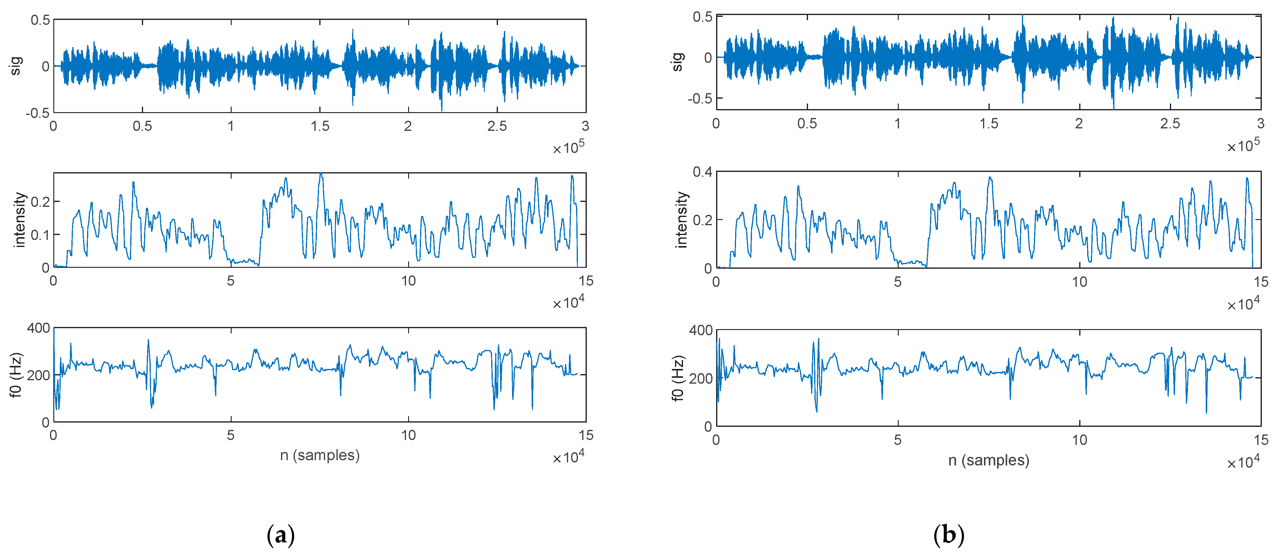
Prosody Analysis
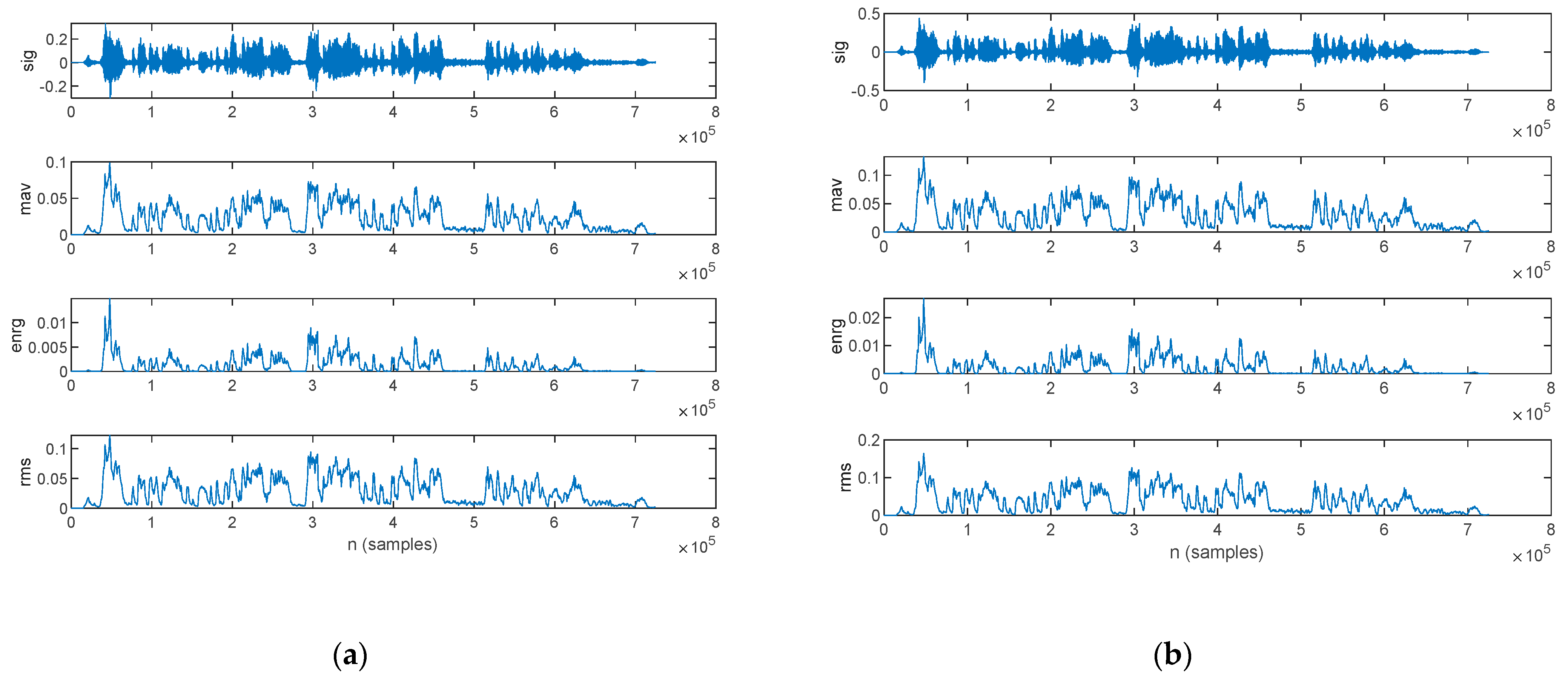
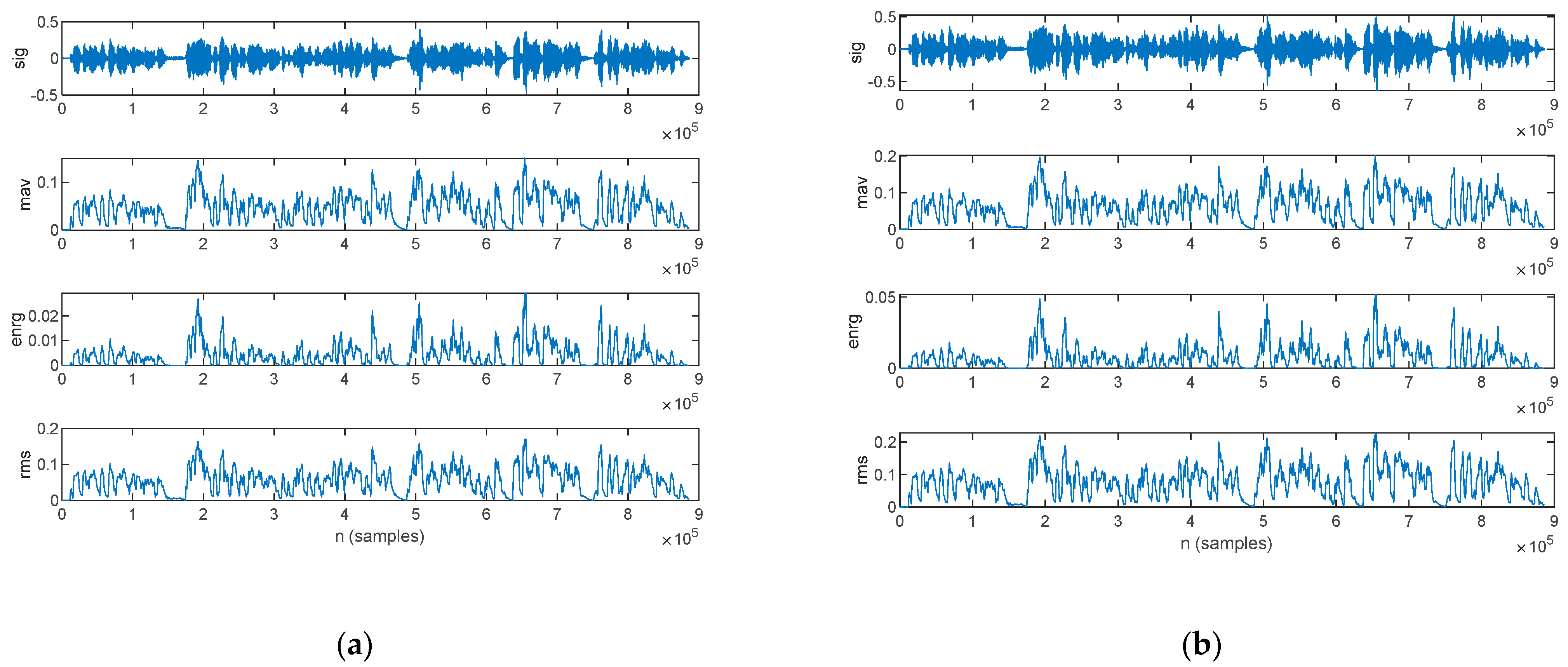
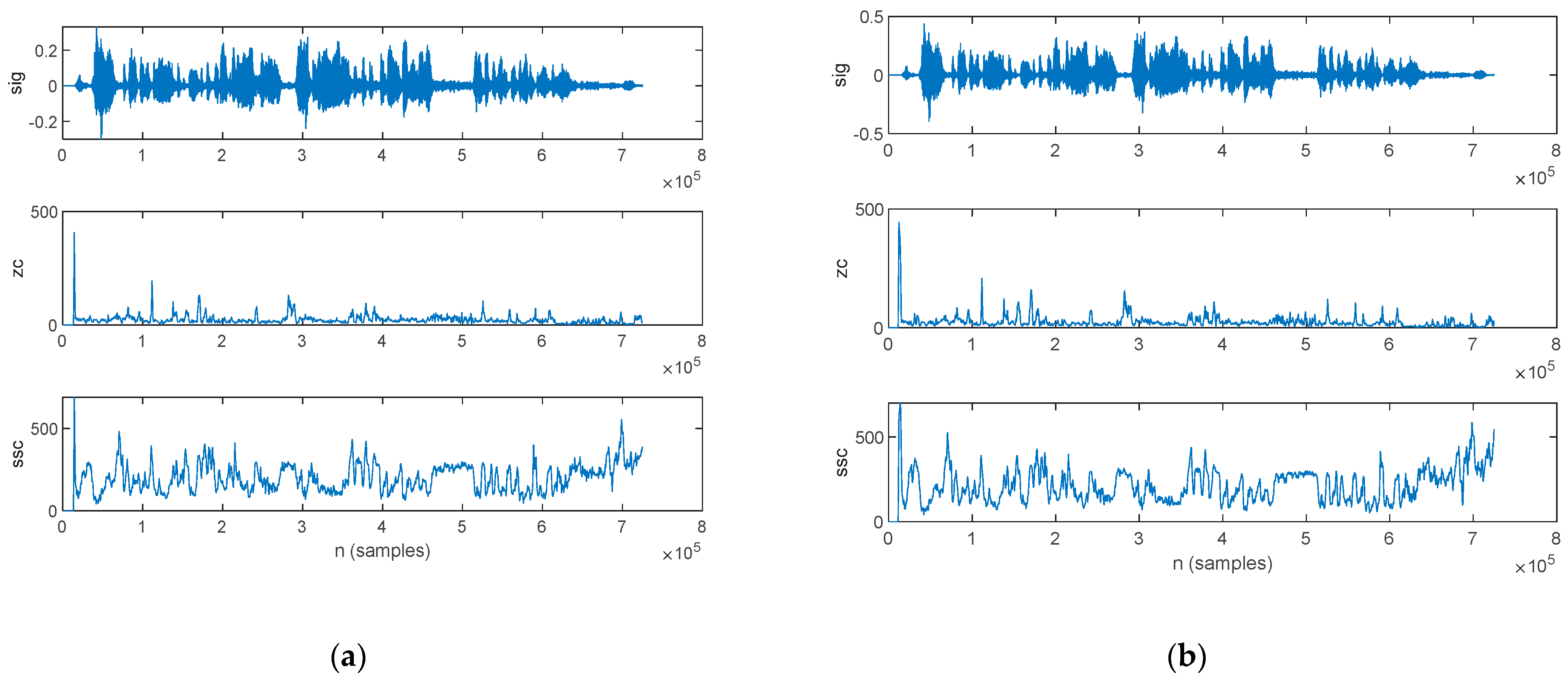
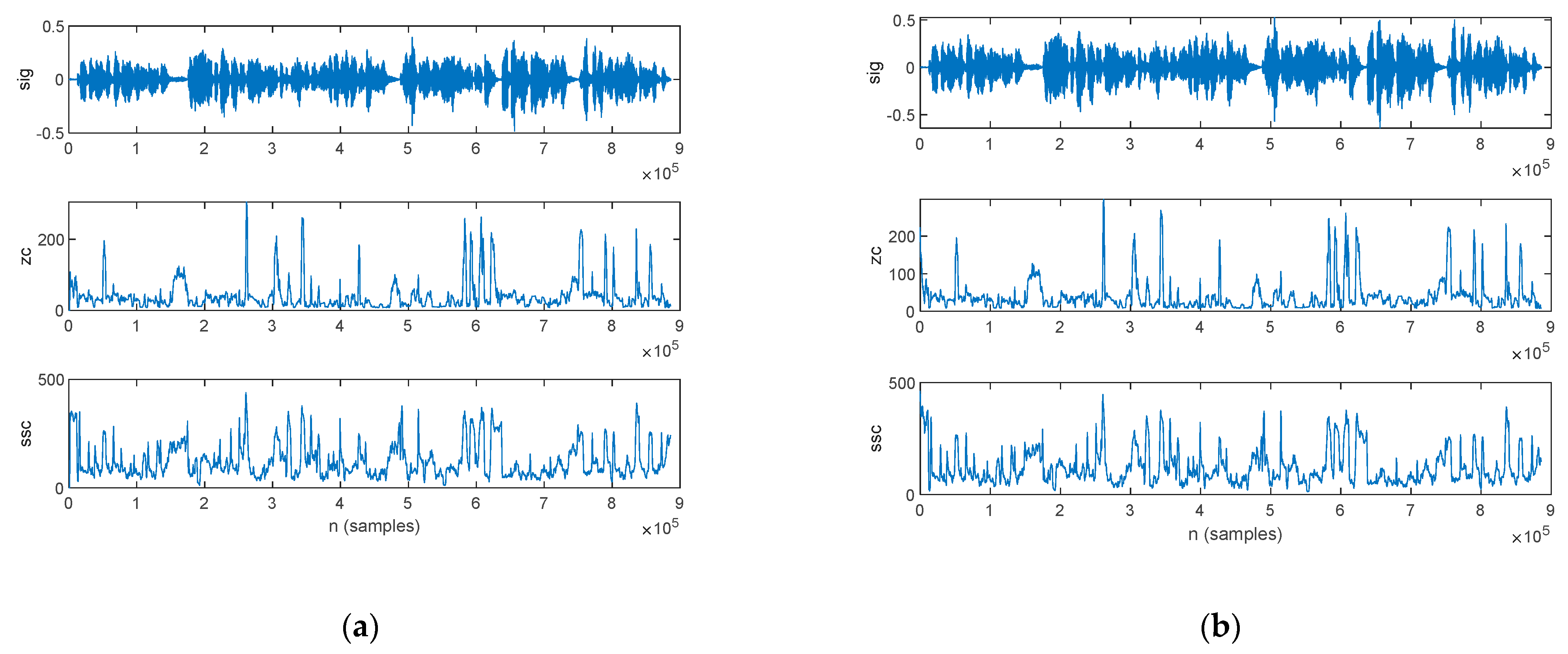
Time-Domain Analysis
Frequency-Domain Analysis
LPC Analysis
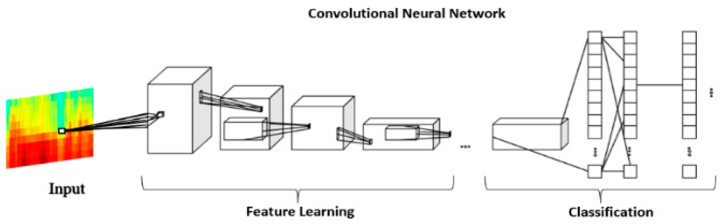
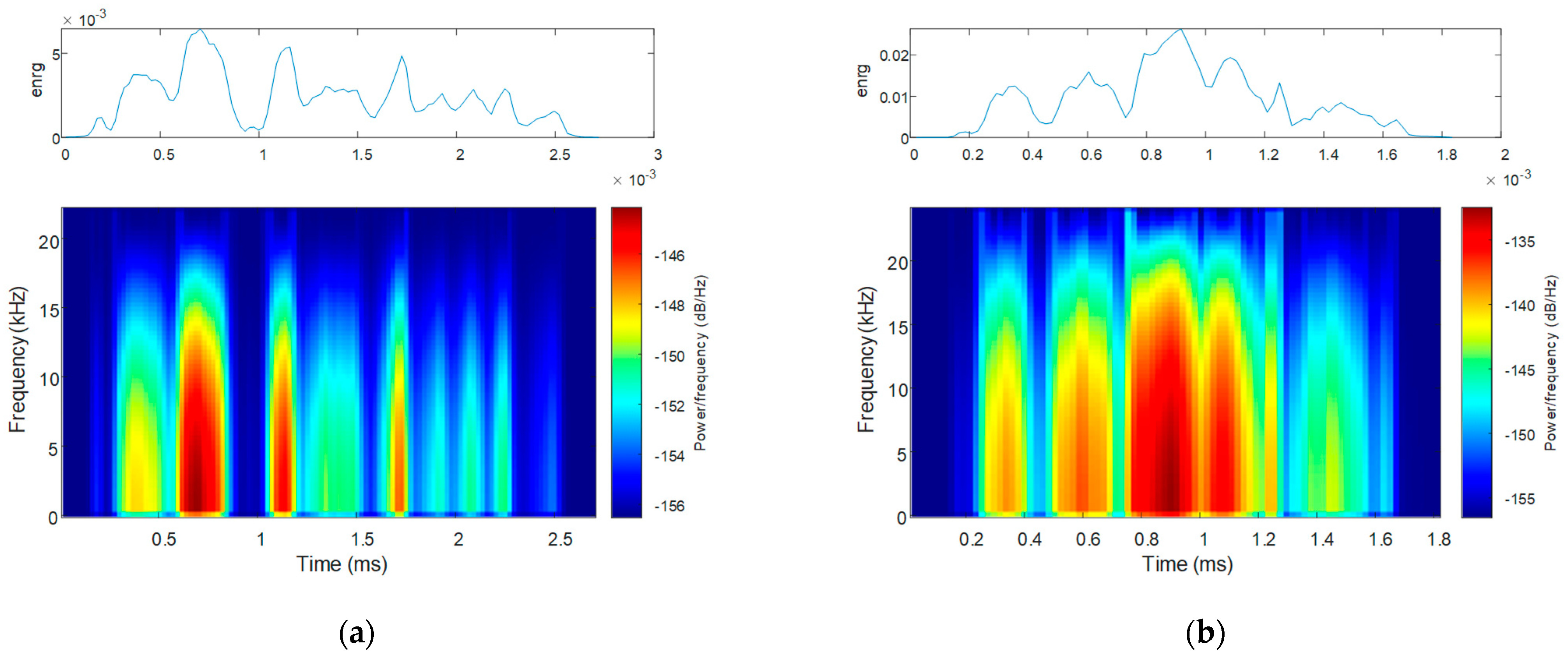
2.2.3. CNN-Based Spectrogram Classification
3. Results
3.1. Wiener Filter Performance Evaluation
3.2. Feature Extraction for Parkinsonian Speech Assessment
3.2.1. Phonological Analysis
3.2.2. Prosody Analysis
3.2.3. Time-Domain Analysis
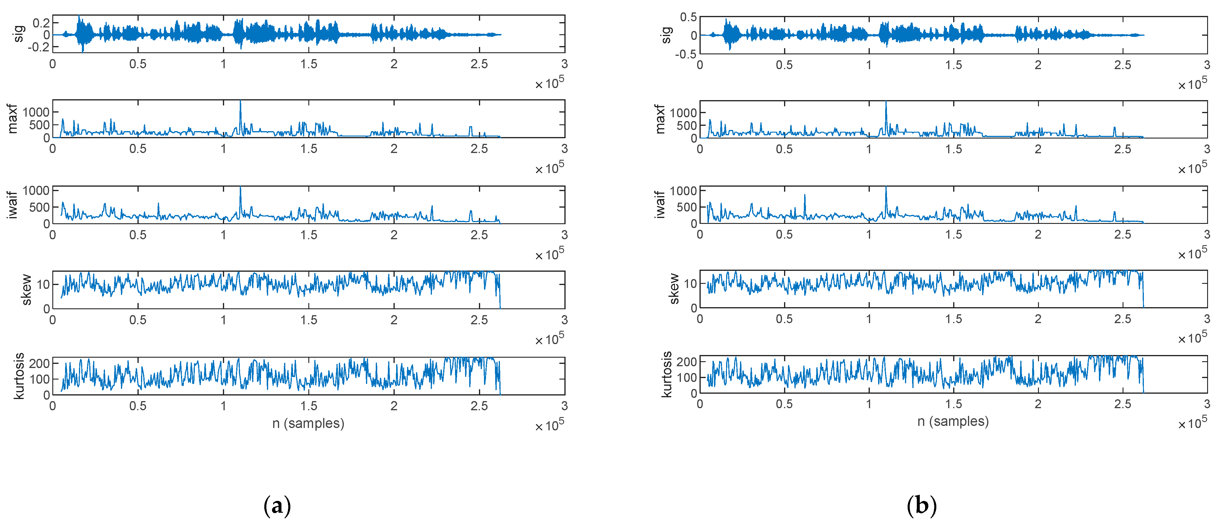
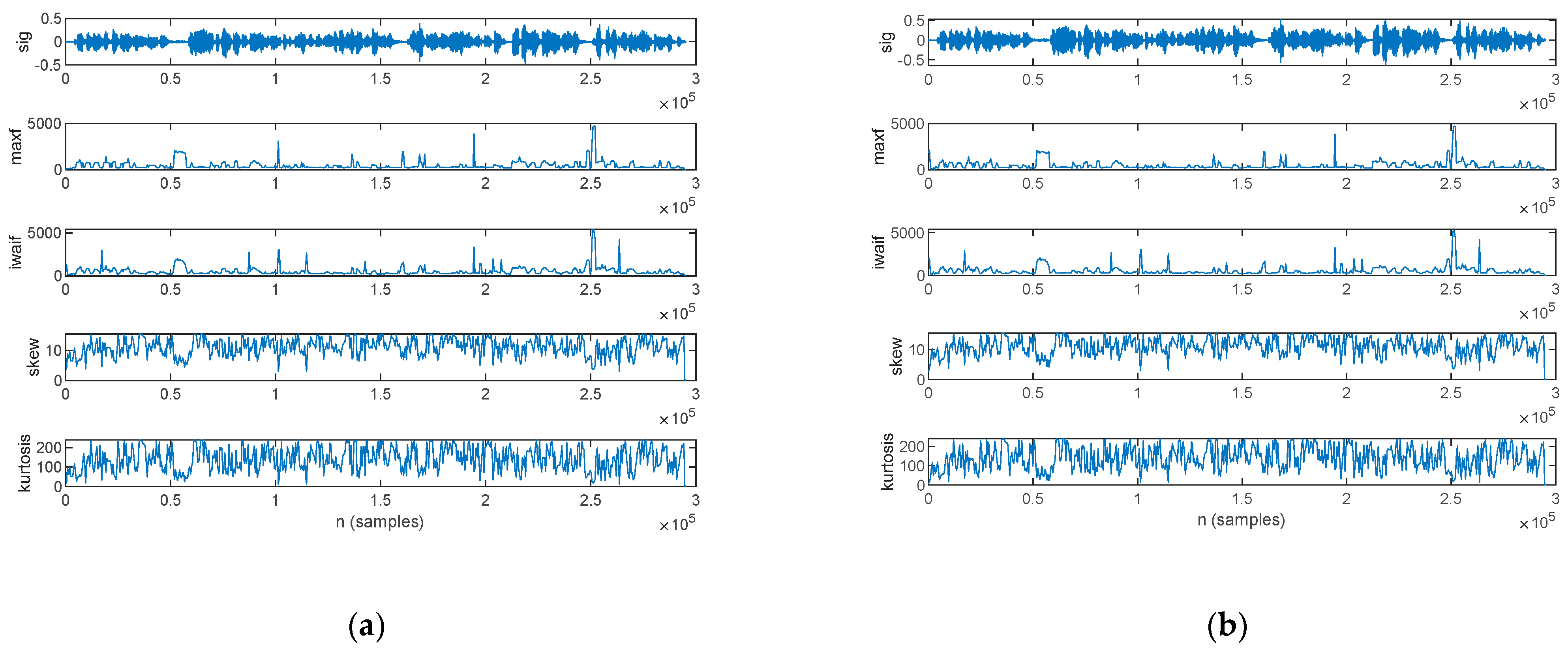
3.2.4. Frequency-Domain Analysis
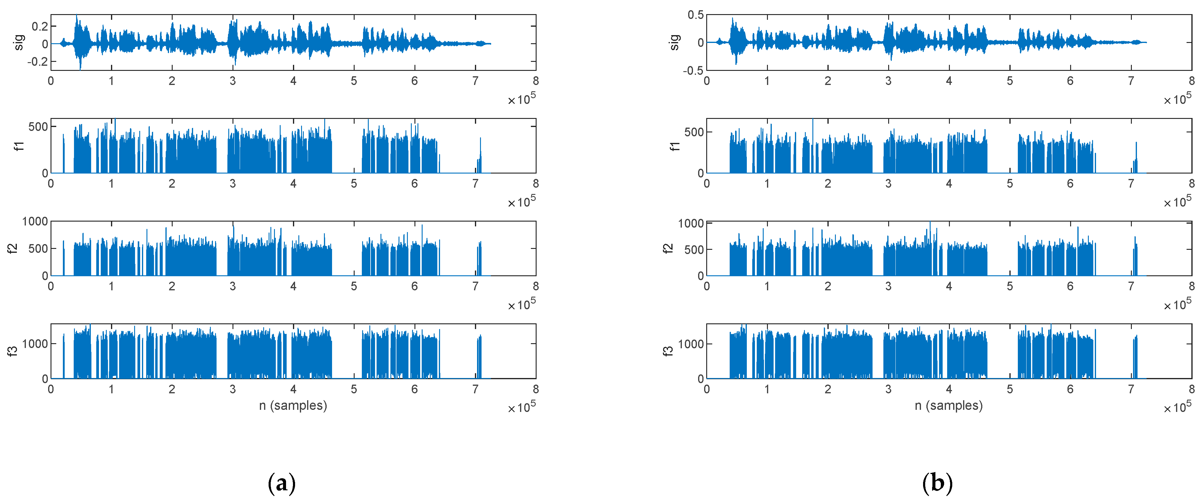
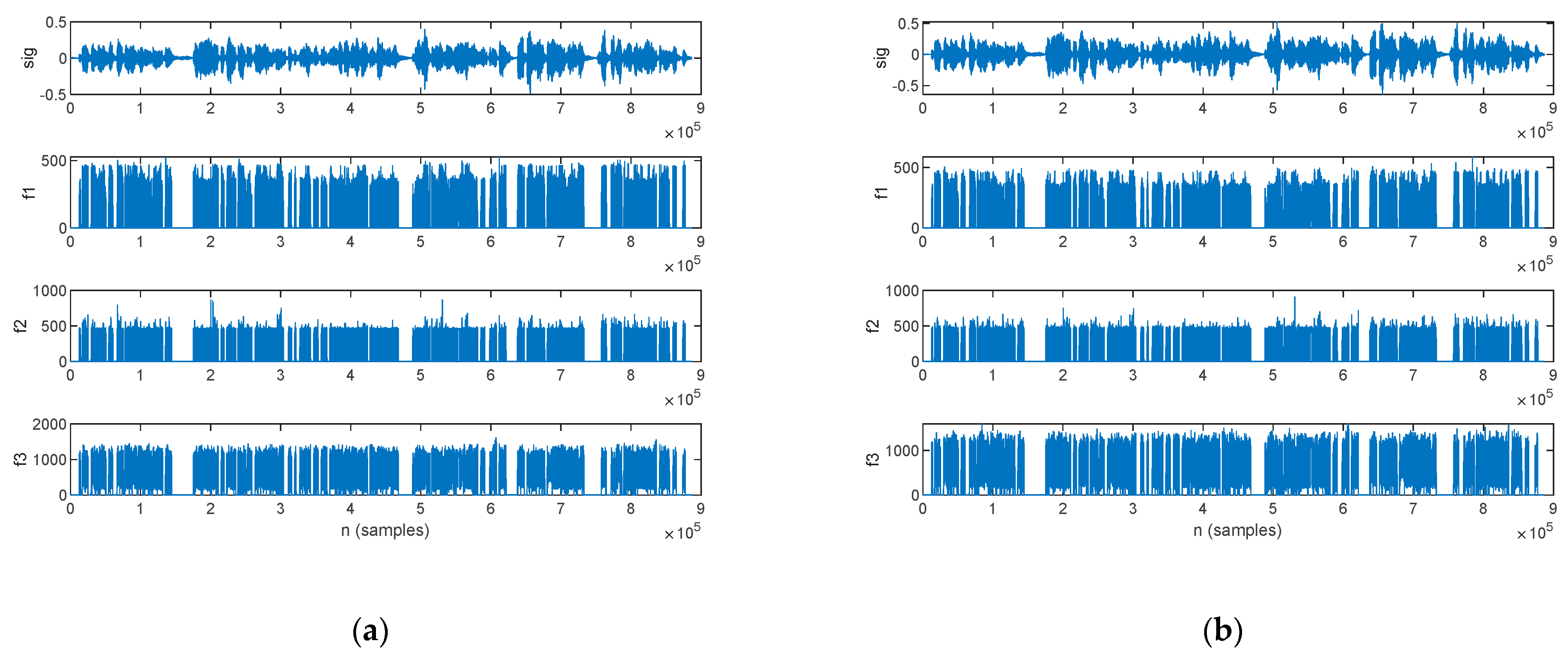
3.2.5. LPC Analysis
3.3. CNN-Based Spectrogram Classification
4. Discussion
4.1. Speech Enhancement and Fidelity Measures
4.2. Feature Extraction for Parkinsonian Speech Assessment
4.2.1. Phonology Analysis
4.2.2. Prosody Analysis
4.2.3. Time-Domain Analysis
4.2.4. Frequency-Domain Analysis
4.2.5. LPC Analysis
4.3. CNN-Based Spectrogram Classification
4.4. Limitations
5. Conclusions
Author Contributions
Funding
Institutional Review Board Statement
Informed Consent Statement
Data Availability Statement
Conflicts of Interest
Appendix A
Appendix A.1. Wiener Filter Performance Evaluation

| ID | SNR (dB) Original Signal | SNR (dB) Filtered Signal | SNRI | MSE |
|---|---|---|---|---|
| PD 1 | 43.1 | 43.2 | 0.1 | 2.29 × 10⁻⁴ |
| PD 2 | 46.3 | 50 | 3.7 | 2.27 × 10⁻⁴ |
| PD 3 | 44.2 | 48.3 | 4.1 | 7.32 × 10⁻⁵ |
| PD 4 | 43.5 | 43.7 | 0.2 | 2.58 × 10⁻⁴ |
| PD 5 | 44.9 | 50.4 | 5.5 | 1.5 × 10⁻⁴ |
| PD 6 | 42.4 | 47.8 | 5.4 | 3.81 × 10⁻⁴ |
| PD 7 | 36.4 | 42.6 | 6.2 | 8.42 × 10⁻⁴ |
| PD 8 | 31.8 | 34.8 | 3 | 3.68 × 10⁻⁴ |
| PD 9 | 46 | 49.3 | 3.3 | 2.47 × 10⁻⁴ |
| PD 10 | 81 | 81.1 | 0.1 | 1.19 × 10⁻⁴ |
| PD 11 | 58.2 | 62.9 | 4.7 | 8.94 × 10⁻⁴ |
| PD 12 | 44.2 | 50.9 | 6.7 | 2.28 × 10⁻⁴ |
| PD 13 | 9.7 | 11.4 | 1.7 | 2.81 × 10⁻⁴ |
| PD 14 | 16.1 | 24.7 | 8.6 | 6.5 × 10⁻⁴ |
| PD 15 | 26.3 | 33.3 | 7 | 1.94 × 10⁻⁴ |
| PD 16 | 15 | 20.9 | 5.9 | 6.93 × 10⁻⁴ |
| Statistics | 39.3 ± 17.4 | 43.5 ± 16.5 | 4.1 ± 2.6 | 2.8 × 10⁻⁴ ± 2.2 × 10⁻⁴ |
| HC 1 | 24 | 31.3 | 7.3 | 3.55 × 10⁻⁴ |
| HC 2 | 38.1 | 44.3 | 6.2 | 4.67 × 10⁻⁴ |
| HC 3 | 33.7 | 41.8 | 8.1 | 3.47 × 10⁻⁴ |
| HC 4 | 27.2 | 28.6 | 1.4 | 3.81 × 10⁻⁴ |
| HC 5 | 42.5 | 46.8 | 4.3 | 1.68 × 10⁻⁴ |
| HC 6 | 32.2 | 39 | 6.8 | 5.8 × 10⁻⁴ |
| HC 7 | 33.5 | 35.4 | 1.9 | 7.49 × 10⁻⁴ |
| HC 8 | 44.1 | 49.5 | 5.4 | 3.35 × 10⁻⁴ |
| HC 9 | 28.2 | 32.3 | 4.1 | 1.2 × 10⁻³ |
| HC 10 | 26.3 | 28.4 | 2.1 | 3.79 × 10⁻⁴ |
| HC 11 | 51.7 | 55 | 3.3 | 6.67 × 10⁻⁴ |
| Statistics | 34.7 ± 8.6 | 39.3 ± 8.9 | 4.6 ± 2.3 | 5.1 × 10⁻⁴ ± 2.8 × 10⁻⁴ |
Appendix A.2. Feature Extraction for Parkinsonian Speech Assessment
Appendix A.2.1. Phonological Analysis
| ID | Original Signal | Filtered Signal | ||||||
|---|---|---|---|---|---|---|---|---|
| nuttering | npause | rspeech | tpause | nuttering | npause | rspeech | tpause | |
| PD 1 | 13 | 12 | 47.4 | 35 | 7 | 6 | 25.6 | 1.8 |
| PD 2 | 19 | 18 | 49.7 | 7.5 | 14 | 13 | 36.6 | 7 |
| PD 3 | 17 | 16 | 49.1 | 8.4 | 14 | 13 | 41.1 | 7.7 |
| PD 4 | 6 | 5 | 35.2 | 1.5 | 5 | 4 | 29.4 | 1.4 |
| PD 5 | 7 | 6 | 24.6 | 4.2 | 7 | 6 | 24.6 | 4 |
| PD 6 | 20 | 19 | 42.7 | 10.7 | 17 | 16 | 36.3 | 10.1 |
| PD 7 | 13 | 12 | 34.1 | 12.2 | 13 | 12 | 32.1 | 11.5 |
| PD 8 | 10 | 9 | 34 | 5.7 | 9 | 8 | 24.9 | 5.2 |
| PD 9 | 11 | 10 | 43.8 | 3.5 | 10 | 9 | 39.8 | 3.2 |
| PD 10 | 14 | 13 | 36.7 | 7.1 | 14 | 13 | 36.7 | 5.8 |
| PD 11 | 7 | 6 | 38.2 | 2.8 | 7 | 6 | 8.2 | 2.7 |
| PD 12 | 10 | 9 | 32.26 | 6.6 | 9 | 8 | 29 | 6.2 |
| PD 13 | 8 | 7 | 28.5 | 3.6 | 9 | 8 | 32 | 3.2 |
| PD 14 | 12 | 11 | 33.4 | 3 | 14 | 13 | 39 | 5.7 |
| PD 15 | 19 | 18 | 48.2 | 7.5 | 18 | 17 | 45.6 | 6.1 |
| PD 16 | 36 | 35 | 52 | 13.4 | 34 | 33 | 49.1 | 11.5 |
| Statistics | 13.9 ± 7.4 | 12.9 ± 7.4 | 39.4 ± 8.3 | 8.3 ± 7.9 | 12.6 ± 6.9 | 11.6 ± 6.9 | 33.1 ± 9.8 | 5.8 ± 3.2 |
| HC 1 | 6 | 5 | 19.8 | 5.2 | 8 | 7 | 24.2 | 5 |
| HC 2 | 4 | 3 | 16.2 | 1.3 | 4 | 3 | 16.2 | 1 |
| HC 3 | 5 | 4 | 21.6 | 2.1 | 6 | 5 | 25.1 | 2 |
| HC 4 | 13 | 12 | 34.3 | 4.4 | 12 | 11 | 34.3 | 4.2 |
| HC 5 | 12 | 11 | 50 | 1.9 | 10 | 9 | 35.7 | 1.7 |
| HC 6 | 12 | 11 | 44.7 | 5.6 | 8 | 7 | 30.7 | 5 |
| HC 7 | 9 | 8 | 28 | 8.9 | 9 | 8 | 28 | 8.6 |
| HC 8 | 18 | 17 | 51.5 | 6.2 | 17 | 16 | 49 | 5.8 |
| HC 9 | 9 | 8 | 29.6 | 3.4 | 7 | 6 | 23.7 | 3.3 |
| HC 10 | 8 | 7 | 30.9 | 3.5 | 7 | 6 | 27.4 | 3.1 |
| HC 11 | 7 | 6 | 20.8 | 7.6 | 7 | 6 | 20.8 | 7.3 |
| Statistics | 9.4 ± 4.1 | 8.4 ± 4.1 | 31.6 ± 12.3 | 4.6 ± 2.4 | 8.6 ± 3.5 | 7.6 ± 3.5 | 28.6 ± 8.8 | 4.3 ± 2.4 |
Appendix A.2.2. Prosody Analysis
| ID | Original Signal | Filtered Signal | ||||||
|---|---|---|---|---|---|---|---|---|
| µ(I) | σ(I) | µ(f0) | σ(f0) | µ(I) | σ(I) | µ(f0) | σ(f0) | |
| PD 1 | 0.075 | 0.091 | 113.2 | 56.6 | 0.076 | 0.093 | 121.12 | 72.18 |
| PD 2 | 0.137 | 0.159 | 232.8 | 58.2 | 0.135 | 0.157 | 234.02 | 57.3 |
| PD 3 | 0.111 | 0.122 | 152.4 | 36.4 | 0.111 | 0.122 | 155.27 | 37.83 |
| PD 4 | 0.105 | 0.118 | 138.6 | 22.5 | 0.106 | 0.119 | 138.62 | 23.8 |
| PD 5 | 0.052 | 0.073 | 140.3 | 66.1 | 0.069 | 0.097 | 150.86 | 69.46 |
| PD 6 | 0.097 | 0.122 | 146.6 | 29.9 | 0.097 | 0.121 | 147.85 | 31.11 |
| PD 7 | 0.143 | 0.156 | 127.3 | 47 | 0.144 | 0.157 | 128.63 | 44.6 |
| PD 8 | 0.077 | 0.093 | 163.6 | 78.7 | 0.081 | 0.096 | 161.31 | 62.25 |
| PD 9 | 0.119 | 0.141 | 120.3 | 36.4 | 0.12 | 0.143 | 120.98 | 36.67 |
| PD 10 | 0.074 | 0.091 | 103.1 | 60.2 | 0.072 | 0.09 | 102.87 | 59.83 |
| PD 11 | 0.05 | 0.07 | 227.5 | 57.2 | 0.07 | 0.093 | 232.98 | 53.89 |
| PD 12 | 0.02 | 0.03 | 136 | 57.9 | 0.03 | 0.041 | 148.47 | 69.2 |
| PD 13 | 0.025 | 0.035 | 196.3 | 82.6 | 0.033 | 0.045 | 206.25 | 79.66 |
| PD 14 | 0.04 | 0.06 | 135.3 | 64.2 | 0.06 | 0.081 | 160.64 | 78.94 |
| PD 15 | 0.02 | 0.027 | 184 | 105.2 | 0.024 | 0.036 | 190.16 | 102.28 |
| PD 16 | 0.02 | 0.025 | 202.2 | 93.5 | 0.024 | 0.034 | 211.98 | 86.7 |
| Statistics | 0.07 ± 0.04 | 0.09 ± 0.05 | 157.5 ± 39.8 | 59.5 ± 22.7 | 0.07 ± 0.04 | 0.09 ± 0.04 | 163 ± 40.4 | 60.4 ± 21.7 |
| Male statistics | 0.08 ± 0.04 | 0.1 ± 0.04 | 138.8 ± 33.9 | 49.8 ± 15.2 | 0.08 ± 0.03 | 0.1 ± 0.03 | 145.3 ± 35.4 | 54 ± 19 |
| Female statistics | 0.07 ± 0.05 | 0.08 ± 0.06 | 188.6 ± 18.8 | 75.8 ± 24.9 | 0.07 ± 0.05 | 0.08 ± 0.05 | 193.2 ± 30.5 | 71 ± 23.1 |
| HC 1 | 0.077 | 0.09 | 155.04 | 65.7 | 0.077 | 0.088 | 155.59 | 63.36 |
| HC 2 | 0.113 | 0.113 | 243.6 | 37.3 | 0.144 | 0.115 | 245.08 | 35.01 |
| HC 3 | 0.102 | 0.112 | 235.2 | 34.5 | 0.1 | 0.11 | 237.23 | 32.35 |
| HC 4 | 0.095 | 0.107 | 172.6 | 38.4 | 0.097 | 0.111 | 178.68 | 46.01 |
| HC 5 | 0.12 | 0.134 | 180.8 | 47.2 | 0.12 | 0.134 | 180.89 | 44.81 |
| HC 6 | 0.075 | 0.096 | 128.9 | 46.1 | 0.075 | 0.098 | 131.12 | 64.72 |
| HC 7 | 0.07 | 0.09 | 203 | 98.3 | 0.076 | 0.098 | 203.31 | 45.85 |
| HC 8 | 0.08 | 0.104 | 156.9 | 45 | 0.081 | 0.106 | 158.45 | 99.16 |
| HC 9 | 0.1 | 0.1 | 131.8 | 50 | 0.096 | 0.103 | 133.56 | 49.14 |
| HC 10 | 0.08 | 0.1 | 160.1 | 64.3 | 0.08 | 0.099 | 161.89 | 65.58 |
| HC 11 | 0.1 | 0.121 | 152 | 53.9 | 0.099 | 0.121 | 152.1 | 54.05 |
| Statistics | 0.09 ± 0.02 | 0.1 ± 0.01 | 174.5 ± 38.2 | 48.7 ± 23.2 | 0.09 ± 0.02 | 0.1 ± 0.01 | 176.38.2 | 54.5 ± 18.5 |
| Male statistics | 0.08 ± 0.01 | 0.1 ± 0.01 | 150.9 ± 17.1 | 44.1 ± 22.1 | 0.08 ± 0.01 | 0.1 ± 0.01 | 153.2 ± 18.1 | 64.7 ± 18.9 |
| Female statistics | 0.09 ± 0.02 | 0.01 ± 0.01 | 202.9 ± 38 | 54.2 ± 25.8 | 0.1 ± 0.03 | 0.1 ± 0.01 | 203.7 ± 38.8 | 42.4 ± 8.9 |
Appendix A.2.3. Time-Domain Analysis
| ID | Original Signal | Filtered Signal | ||||||||||
|---|---|---|---|---|---|---|---|---|---|---|---|---|
| µ(mav) | σ(mav) | µ(enrg) | σ(enrg) | µ(rms) | σ(rms) | µ(mav) | σ(mav) | µ(enrg) | σ(enrg) | µ(rms) | σ(rms) | |
| PD 1 | 28 | 17 | 0.2 | 0.2 | 35 | 21 | 34 | 23 | 0.3 | 0.3 | 43 | 30 |
| PD 2 | 33 | 25 | 0.2 | 0.3 | 39 | 29 | 43 | 34 | 0.4 | 0.6 | 50 | 39 |
| PD 3 | 22 | 12 | 0.1 | 0.1 | 26 | 15 | 28 | 17 | 0.2 | 0.1 | 34 | 20 |
| PD 4 | 33 | 23 | 0.3 | 0.3 | 42 | 29 | 44 | 31 | 0.5 | 0.5 | 55 | 39 |
| PD 5 | 52 | 52 | 0.8 | 1.2 | 64 | 63 | 70 | 69 | 1.4 | 2.2 | 86 | 84 |
| PD 6 | 35 | 29 | 0.3 | 0.4 | 41 | 34 | 46 | 59 | 1.7 | 4.9 | 57 | 116 |
| PD 7 | 24 | 14 | 0.1 | 0.1 | 28 | 16 | 31 | 19 | 0.2 | 0.2 | 37 | 22 |
| PD 8 | 41 | 29 | 0.4 | 0.5 | 50 | 35 | 53 | 39 | 0.7 | 0.8 | 65 | 48 |
| PD 9 | 29 | 20 | 0.2 | 0.2 | 36 | 25 | 38 | 27 | 0.3 | 0.4 | 47 | 34 |
| PD 10 | 21 | 13 | 0.1 | 0.1 | 27 | 17 | 27 | 18 | 0.2 | 0.2 | 34 | 23 |
| PD 11 | 7 | 55 | 1 | 1.2 | 79 | 61 | 93 | 75 | 1.8 | 2.2 | 105 | 83 |
| PD 12 | 33 | 22 | 0.2 | 0.2 | 39 | 25 | 43 | 30 | 0.4 | 0.4 | 51 | 34 |
| PD 13 | 33 | 24 | 0.2 | 0.4 | 39 | 29 | 40 | 33 | 0.4 | 0.7 | 48 | 39 |
| PD 14 | 50 | 43 | 0.6 | 0.9 | 61 | 51 | 73 | 60 | 1.3 | 1.8 | 88 | 71 |
| PD 15 | 25 | 23 | 0.2 | 0.4 | 29 | 26 | 32 | 31 | 0.3 | 0.6 | 37 | 34 |
| PD 16 | 26 | 23 | 0.1 | 0.4 | 31 | 26 | 32 | 26 | 0.2 | 0.4 | 38 | 30 |
| Statistics | 36 ± 13 | 27 ± 13 | 0.3 ± 0.3 | 0.5 ± 0.4 | 43 ± 15 | 32 ± 15 | 47 ± 18 | 38 ± 18 | 0.7 ± 0.6 | 0.4 ± 0.1 | 56 ± 21 | 48 ± 28 |
| Male statistics | 39 ± 15 | 31 ± 16 | 0.4 ± 0.3 | 0.5 ± 0.4 | 47 ± 17 | 36 ± 18 | 52 ± 22 | 44 ± 22 | 0.9 ± 0.7 | 0.6 ± 0.2 | 63 ± 24 | 57 ± 32 |
| Female statistics | 3 ± 0.7 | 23 ± 6 | 0.2 ± 0.1 | 0.4 ± 0.1 | 36 ± 0.9 | 27 ± 7 | 38 ± 9 | 30 ± 8 | 0.4 ± 0.2 | 0.5 ± 0.3 | 45 ± 12 | 35 ± 10 |
| HC 1 | 39 | 29 | 0.3 | 0.5 | 47 | 34 | 52 | 39 | 0.6 | 0.9 | 63 | 0.045 |
| HC 2 | 49 | 28 | 0.5 | 0.5 | 59 | 34 | 65 | 39 | 0.8 | 0.8 | 78 | 0.045 |
| HC 3 | 42 | 31 | 0.4 | 0.6 | 49 | 36 | 55 | 43 | 0.7 | 1.1 | 66 | 0.048 |
| HC 4 | 41 | 29 | 0.4 | 0.5 | 49 | 34 | 52 | 39 | 0.6 | 0.9 | 63 | 0.046 |
| HC 5 | 26 | 18 | 0.2 | 0.2 | 32 | 22 | 35 | 25 | 0.3 | 0.3 | 43 | 0.029 |
| HC 6 | 45 | 36 | 0.5 | 0.7 | 58 | 45 | 60 | 48 | 0.9 | 1.3 | 76 | 0.061 |
| HC 7 | 62 | 49 | 1 | 1.4 | 78 | 64 | 82 | 66 | 1.8 | 2.6 | 103 | 0.086 |
| HC 8 | 39 | 30 | 0.4 | 0.5 | 49 | 38 | 50 | 66 | 0.7 | 2.6 | 64 | 0.086 |
| HC 9 | 73 | 47 | 12 | 1.2 | 91 | 58 | 98 | 38 | 2.1 | 0.8 | 121 | 0.047 |
| HC 10 | 37 | 28 | 0.3 | 0.4 | 46 | 35 | 48 | 38 | 0.6 | 0.8 | 61 | 0.047 |
| HC 11 | 59 | 45 | 0.8 | 1.1 | 74 | 55 | 78 | 62 | 1.5 | 1.9 | 98 | 0.075 |
| Statistics | 47 ± 13 | 34 ± 10 | 0.5 ± 0.3 | 0.7 ± 0.4 | 57 ± 17 | 41 ± 13 | 61 ± 18 | 46 ± 13 | 1 ± 0.6 | 1.3 ± 0.8 | 76 ± 23 | 56 ± 19 |
| Male statistics | 46 ± 14 | 33 ± 7 | 0.5 ± 0.3 | 0.6 ± 0.3 | 57 ± 17 | 41 ± 9 | 60 ± 19 | 45 ± 11 | 0.9 ± 0.6 | 1.2 ± 0.7 | 75 ± 23 | 55 ± 16 |
| Female statistics | 48 ± 14 | 34 ± 13 | 0.6 ± 0.3 | 0.8 ± 0.5 | 58 ± 19 | 42 ± 17 | 63 ± 19 | 47 ± 17 | 1 ± 0.6 | 1.3 ± 0.9 | 78 ± 24 | 57 ± 23 |
| ID | Original Signal | Filtered Signal | ||||||
|---|---|---|---|---|---|---|---|---|
| µ(ZC) | σ(ZC) | µ(SSC) | σ(SSC) | µ(ZC) | σ(ZC) | µ(SSC) | σ(SSC) | |
| PD 1 | 22.357 | 16.859 | 182.544 | 74.584 | 22.641 | 18.677 | 196.727 | 82.65 |
| PD 2 | 29.307 | 53.375 | 140.798 | 140.374 | 31.872 | 59.298 | 140.584 | 140.668 |
| PD 3 | 24.325 | 21.144 | 121.928 | 88.092 | 26.712 | 29.402 | 118.478 | 87.19 |
| PD 4 | 28.659 | 29.329 | 181.151 | 126.526 | 29.181 | 30.003 | 183.965 | 128.598 |
| PD 5 | 66.081 | 81.9 | 290.121 | 173.9 | 70.194 | 102.646 | 279.219 | 191.997 |
| PD 6 | 30.005 | 52.14 | 204.257 | 121.608 | 30.947 | 54.477 | 198.394 | 120.823 |
| PD 7 | 23.845 | 40.067 | 148.127 | 109.047 | 24.749 | 41.65 | 142.158 | 107.563 |
| PD 8 | 34.632 | 43.872 | 144.893 | 104.41 | 35.116 | 44.324 | 150.085 | 107.657 |
| PD 9 | 19.442 | 24.564 | 180.573 | 113.788 | 20.094 | 25.974 | 178.236 | 114.469 |
| PD 10 | 29.116 | 39.246 | 195.915 | 108.027 | 29.614 | 41.167 | 203.457 | 110.171 |
| PD 11 | 21.374 | 31.819 | 129.823 | 123.655 | 22.56 | 33.815 | 132.5 | 122.207 |
| PD 12 | 16.494 | 28.891 | 174.101 | 112.079 | 17.197 | 31.203 | 169.326 | 110.657 |
| PD 13 | 16.494 | 33.584 | 174.101 | 88.326 | 30.754 | 39.367 | 134.914 | 93.509 |
| PD 14 | 37.431 | 55.588 | 217.195 | 128.352 | 46.013 | 70.774 | 223.118 | 145.956 |
| PD 15 | 15.75 | 18.996 | 169.841 | 131.924 | 17.229 | 23.741 | 171.263 | 132.151 |
| PD 16 | 34.654 | 18.996 | 206.441 | 131.924 | 37.338 | 57.353 | 199.109 | 116.7 |
| Statistics | 28.1 ± 12.6 | 36.7 ± 18 | 177.7 ± 41.9 | 117.9 ± 24.2 | 30.8 ± 13.4 | 44.2 ± 22 | 174 ± 41.8 | 118.9 ± 23.3 |
| Male statistics | 29.5 ± 14.2 | 40.1 ± 18.9 | 189.8 ± 43.3 | 120.4 ± 24.6 | 31.5 ± 15.8 | 45.5 ± 25.2 | 189.3 ± 41.6 | 122.8 ± 24 |
| Female statistics | 25.9 ± 8.5 | 31.7 ± 14.5 | 159.7 ± 30 | 114.2 ± 23.5 | 29.8 ± 7.1 | 42.2 ± 14.4 | 152.4 ± 28.8 | 113 ± 21.1 |
| HC 1 | 45.747 | 76.733 | 174.158 | 123.921 | 47.013 | 78.947 | 172.795 | 125.428 |
| HC 2 | 38.708 | 42.538 | 118.255 | 76.937 | 38.446 | 41.955 | 117.145 | 76.903 |
| HC 3 | 30.326 | 38.703 | 154.189 | 93.201 | 30.003 | 40.942 | 143.291 | 96.501 |
| HC 4 | 40.387 | 62.869 | 187.823 | 100.331 | 41.831 | 66.345 | 182.848 | 109.791 |
| HC 5 | 32 | 38.802 | 90.089 | 61.733 | 34.475 | 43.336 | 99.189 | 65.526 |
| HC 6 | 24.872 | 27.766 | 92.931 | 52.635 | 26.421 | 31.123 | 101.402 | 57.502 |
| HC 7 | 39.459 | 40.397 | 124.723 | 55.802 | 41.166 | 42.695 | 132.305 | 58.475 |
| HC 8 | 27.968 | 28.14 | 84.773 | 64.632 | 29.544 | 42.695 | 92.793 | 58.475 |
| HC 9 | 42.379 | 58.031 | 184.803 | 122.555 | 42.955 | 36.452 | 184.222 | 54.428 |
| HC 10 | 35.396 | 34.743 | 93.197 | 50.388 | 36.469 | 36.452 | 96.985 | 54.428 |
| HC 11 | 42.988 | 77.642 | 195.069 | 133.854 | 43.701 | 78.549 | 197.261 | 135.084 |
| Statistics | 36.4 ± 6.8 | 47.9 ± 18 | 136.4 ± 43.8 | 85.1 ± 31.2 | 37.4 ± 6.7 | 49.5 ± 17.1 | 138.2 ± 39.9 | 81.1 ± 30.3 |
| Male statistics | 36.1 ± 8.3 | 48 ± 20.6 | 136.6 ± 50.7 | 85.7 ± 34.1 | 37.4 ± 8 | 48.7 ± 19.3 | 138.5 ± 45.7 | 76.7 ± 32.1 |
| Female statistics | 36.7 ± 5.3 | 47.6 ± 16.9 | 136.5 ± 39.9 | 84.3 ± 31.3 | 37.6 ± 5.4 | 49.5 ± 16.3 | 137.8 ± 37.1 | 86.5 ± 30.7 |
Appendix A.2.4. Frequency-Domain Analysis
| ID | Original Signal | Filtered Signal | ||||||
|---|---|---|---|---|---|---|---|---|
| µ(maxf) | µ(waf) | µ(skw) | µ(kur) | µ(maxf) | µ(waf) | µ(skw) | µ(kur) | |
| PD 1 | 209.8221 | 224.8454 | 9.976358 | 117.5921 | 190.2661 | 209.5559 | 10.33465 | 125.1718 |
| PD 2 | 360.1689 | 416.25 | 11.92247 | 159.6 | 414.8776 | 444.9981 | 11.83087 | 157.4186 |
| PD 3 | 370.1667 | 366.0654 | 9.967189 | 117.7195 | 375.2765 | 383.3179 | 9.904568 | 116.8925 |
| PD 4 | 250.2299 | 306.0685 | 10.05182 | 119.875 | 267.008 | 305.6195 | 10.13883 | 121.6912 |
| PD 5 | 302.4605 | 370.1943 | 9.733266 | 113.4279 | 300.2343 | 374.7697 | 10.01356 | 118.778 |
| PD 6 | 230.2874 | 260.1802 | 12.05196 | 161.9582 | 230.490524 | 268.8687 | 12.06773 | 162.2545 |
| PD 7 | 220.8475 | 253.263 | 10.69389 | 130.4106 | 223.762915 | 250.1917 | 10.76735 | 132.0026 |
| PD 8 | 345.9367 | 411.2698 | 10.22188 | 123.6549 | 355.175689 | 417.4254 | 10.17484 | 122.818 |
| PD 9 | 182.4607 | 208.4106 | 10.10069 | 119.5384 | 184.348562 | 210.2118 | 10.139 | 120.2532 |
| PD 10 | 305.2498 | 319.7704 | 9.385109 | 106.0929 | 296.426479 | 327.8041 | 9.545114 | 109.7087 |
| PD 11 | 249.8765 | 277.7127 | 13.11219 | 185.5506 | 262.681159 | 289.9209 | 13.00803 | 183.6191 |
| PD 12 | 146.2178 | 154.7583 | 11.97501 | 158.6683 | 144.605475 | 157.4248 | 11.97299 | 158.6024 |
| PD 13 | 315.6509 | 354.7091 | 10.87591 | 136.1331 | 365.054945 | 395.4144 | 10.86759 | 136.3212 |
| PD 14 | 298.2712 | 336.0759 | 10.39996 | 125.5157 | 430.044276 | 463.8346 | 10.22208 | 122.7967 |
| PD 15 | 219.5424 | 235.0433 | 11.66939 | 152.9737 | 225.228311 | 233.9798 | 11.6668 | 153.0658 |
| PD 16 | 433.1558 | 464.4558 | 11.40796 | 149.6136 | 447.3 | 508.7318 | 11.26647 | 146.6707 |
| Statistics | 277.5 ± 76.9 | 309.9 ± 85.2 | 10.8 ± 1 | 136.1 ± 22.5 | 294.5 ± 94 | 327.6 ± 103.3 | 10.9 ± 1 | 136.7 ± 21 |
| Male statistics | 239.6 ± 53.9 | 271.1 ± 63.1 | 10.7 ± 1.2 | 133.9 ± 25.9 | 253 ± 77 | 285.8 ± 85.4 | 10.8 ± 1.1 | 135.5 ± 24.1 |
| Female statistics | 340.8 ± 70.9 | 374.6 ± 78.9 | 11 ± 0.8 | 139.9 ± 16.9 | 363.8 ± 76.1 | 397.3 ± 91.6 | 11 ± 0.8 | 138.9 ± 16.5 |
| HC 1 | 623.3607 | 657.5876 | 9.915721 | 118.046 | 647.812359 | 682.7459 | 9.895411 | 117.3672 |
| HC 2 | 477.2542 | 522.7215 | 11.13494 | 142.5209 | 451.206897 | 516.0038 | 11.10386 | 141.5863 |
| HC 3 | 301.9284 | 349.3909 | 11.5549 | 149.9868 | 288.343558 | 345.2166 | 11.67933 | 152.7823 |
| HC 4 | 343.8331 | 397.1155 | 10.73022 | 132.7825 | 370.254314 | 428.8957 | 10.85112 | 135.3927 |
| HC 5 | 473.8431 | 510.7556 | 10.06492 | 121.1023 | 506.415344 | 553.0855 | 9.929213 | 118.6239 |
| HC 6 | 340.6038 | 380.7002 | 9.451434 | 107.9514 | 358.076225 | 400.7224 | 9.440863 | 107.6968 |
| HC 7 | 641.3078 | 678.6393 | 10.06799 | 120.9231 | 642.514345 | 691.8391 | 10.03913 | 120.6899 |
| HC 8 | 448.7052 | 474.8081 | 10.08178 | 119.5018 | 475.053763 | 496.7997 | 10.04414 | 119.2715 |
| HC 9 | 367.6768 | 403.4554 | 9.790699 | 114.6094 | 376.106195 | 410.718 | 9.844548 | 115.3877 |
| HC 10 | 571.8169 | 627.1641 | 9.956054 | 118.8349 | 588.329839 | 623.486 | 9.8651 | 116.949 |
| HC 11 | 439.9353 | 501.9098 | 10.13185 | 121.2875 | 444.933078 | 498.9354 | 10.14959 | 121.573 |
| Statistics | 457.3 ± 115.9 | 500.4 ± 114.5 | 10.9 ± 1 | 124.3 ± 12.4 | 468.1 ± 199.2 | 513.5 ± 155.5 | 10.3 ± 0.7 | 124.3 ± 13.3 |
| Male statistics | 449.3 ± 122.4 | 490.1 ± 122.6 | 10.9 ± 1.3 | 118.6 ± 8.1 | 469.3 ± 124 | 507.3 ± 199.4 | 10 ± 0.5 | 118.7 ± 9.1 |
| Female statistics | 466.9 ± 121 | 512.7 ± 116.6 | 11 ± 0.8 | 131.2 ± 14 | 466.7 ± 127.5 | 521 ± 124.1 | 10.6 ± 0.8 | 131 ± 15.3 |
| ID | Original Signal | Filtered Signal | ||||||
|---|---|---|---|---|---|---|---|---|
| σ(maxf) | σ(waf) | σ(skw) | σ(kur) | σ(maxf) | σ(waf) | σ(skw) | σ(kur) | |
| PD 1 | 140.8132 | 110.2558 | 2.633903 | 55.30804 | 123.2352 | 109.5277 | 2.743987 | 58.12588 |
| PD 2 | 785.5251 | 789.5384 | 2.994304 | 63.92157 | 989.0715 | 887.1457 | 2.978835 | 63.58607 |
| PD 3 | 258.7677 | 197.0151 | 2.825177 | 57.78512 | 298.5884 | 288.7914 | 2.904553 | 58.90765 |
| PD 4 | 286.0091 | 282.4953 | 2.691118 | 55.13494 | 317.0508 | 263.9887 | 2.731828 | 55.89014 |
| PD 5 | 528.8487 | 544.7161 | 2.818697 | 56.79514 | 536.2376 | 547.2557 | 2.781482 | 56.80749 |
| PD 6 | 607.7036 | 544.687 | 2.760685 | 60.40223 | 623.1119 | 592.8185 | 2.748375 | 60.312 |
| PD 7 | 442.4261 | 451.3987 | 2.440274 | 53.07628 | 459.0798 | 459.009 | 2.424676 | 52.861 |
| PD 8 | 437.354 | 463.7074 | 2.910983 | 59.8237 | 456.3991 | 482.6861 | 2.93604 | 59.88946 |
| PD 9 | 89.73631 | 70.23631 | 2.505477 | 52.43359 | 88.24194 | 77.2381 | 2.538476 | 53.54082 |
| PD 10 | 584.4737 | 458.1556 | 2.729204 | 56.43168 | 588.0268 | 518.4518 | 2.80797 | 58.18234 |
| PD 11 | 253.676 | 264.5755 | 2.713397 | 58.55941 | 305.6971 | 313.7641 | 2.803873 | 60.36714 |
| PD 12 | 62.34063 | 66.32817 | 2.503306 | 56.13981 | 60.54761 | 98.17067 | 2.463561 | 55.52048 |
| PD 13 | 317.5697 | 296.6603 | 2.728088 | 58.53734 | 544.5609 | 494.1021 | 2.76784 | 58.32652 |
| PD 14 | 781.5125 | 698.909 | 2.621361 | 54.91706 | 1089.867 | 990.5238 | 2.743447 | 56.2561 |
| PD 15 | 199.1553 | 255.0108 | 2.662286 | 58.29154 | 255.5855 | 279.8706 | 2.659547 | 58.0698 |
| PD 16 | 1051.378 | 926.1861 | 3.181141 | 67.42014 | 1012.541 | 1020.364 | 3.235481 | 68.03222 |
| Statistics | 426.7 ± 280.8 | 401.2 ± 255.5 | 2.7 ± 0.2 | 57.8 ± 3.8 | 484.2 ± 321.6 | 4634 ± 297.8 | 2.8 ± 0.2 | 58.4 ± 3.7 |
| Male statistics | 377.8 ± 260.3 | 349.2 ± 236.3 | 2.6 ± 0.8 | 55.9 ± 17 | 419.1 ± 323.1 | 380.4 ± 304.7 | 2.7 ± 0.9 | 56.8 ± 18.1 |
| Female statistics | 508.3 ± 338 | 488 ± 303 | 2.9 ± 0.2 | 61 ± 3.8 | 592.8 ± 333 | 575.5 ± 309.8 | 2.9 ± 0.2 | 61.1 ± 3.9 |
| HC 1 | 1410.013 | 1295.124 | 3.047597 | 60.42438 | 1434.005 | 1370.838 | 3.010594 | 60.23597 |
| HC 2 | 600.6572 | 546.8154 | 2.948929 | 62.02396 | 508.5495 | 533.5049 | 2.916 | 61.50816 |
| HC 3 | 317.4417 | 359.8861 | 2.664837 | 58.45661 | 252.831 | 320.5499 | 2.647889 | 57.81285 |
| HC 4 | 709.2429 | 659.4237 | 2.741509 | 56.89116 | 725.7896 | 736.6574 | 2.765028 | 57.35001 |
| HC 5 | 741.7255 | 707.3263 | 3.074998 | 61.17489 | 841.5044 | 806.4467 | 3.18064 | 62.78911 |
| HC 6 | 476.0353 | 457.6013 | 2.816181 | 56.1085 | 531.2828 | 506.766 | 2.814497 | 55.93618 |
| HC 7 | 915.6143 | 873.083 | 3.062648 | 61.8054 | 964.6048 | 903.3665 | 3.124569 | 62.63882 |
| HC 8 | 433.6057 | 445.4268 | 2.558988 | 52.90653 | 538.7827 | 523.2871 | 2.677256 | 54.6878 |
| HC 9 | 469.309 | 410.9073 | 2.850247 | 59.04572 | 398.2593 | 419.0779 | 2.801386 | 58.13629 |
| HC 10 | 731.1745 | 751.7804 | 3.00003 | 60.84957 | 764.2004 | 758.5625 | 3.039602 | 61.60967 |
| HC 11 | 790.7127 | 816.42 | 2.873028 | 57.9772 | 821.1247 | 796.3562 | 2.871022 | 58.41921 |
| Statistics | 690.5 ± 298.5 | 665.8 ± 271.2 | 2.9 ± 0.2 | 58.9 ± 2.8 | 707.4 ± 320.9 | 697.8 ± 289.1 | 59.2 ± 0.2 | 59.2 ± 2.7 |
| Male statistics | 704.9 ± 368.6 | 670 ± 334.7 | 2.8 ± 0.2 | 57.7 ± 3 | 732 ± 369.6 | 719.2 ± 346.4 | 2.9 ± 0.14 | 58 ± 2.6 |
| Female statistics | 673.2 ± 288.6 | 660.7 ± 209.2 | 2.9 ± 0.2 | 60.3 ± 1.9 | 677.7 ± 291 | 672 ± 239.7 | 2.9 ± 0.2 | 60.6 ± 2.4 |
Appendix A.2.5. LPC Analysis
| ID | Original Signal | Filtered Signal | ||||
|---|---|---|---|---|---|---|
| µ(f1) | µ(f2) | µ(f3) | µ(f1) | µ(f2) | µ(f3) | |
| PD 1 | 146.3977 | 356.2246 | 927.9631 | 95.99813 | 215.8823 | 664.4091 |
| PD 2 | 140.5878 | 305.1284 | 846.6479 | 143.1003 | 309.3127 | 853.4781 |
| PD 3 | 116.3885 | 238.901 | 723.2804 | 117.1406 | 241.6413 | 728.9491 |
| PD 4 | 116.3885 | 238.901 | 723.2804 | 112.4424 | 251.6562 | 725.0138 |
| PD 5 | 106.2606 | 244.0261 | 718.9596 | 107.1858 | 246.2775 | 720.2278 |
| PD 6 | 117.6647 | 295.6761 | 806.0591 | 128.2465 | 321.9942 | 865.6273 |
| PD 7 | 126.7025 | 318.2057 | 858.2249 | 124.9557 | 246.3748 | 721.9826 |
| PD 8 | 125.9183 | 249.031 | 725.5743 | 118.7285 | 290.2411 | 808.252 |
| PD 9 | 118.2062 | 286.9403 | 799.7578 | 92.24254 | 199.7526 | 636.9858 |
| PD 10 | 90.98081 | 195.1003 | 631.759 | 167.9252 | 397.4367 | 1007.766 |
| PD 11 | 168.3419 | 398.1365 | 1008.629 | 128.3763 | 346.5467 | 900.6316 |
| PD 12 | 127.7762 | 344.6129 | 898.1218 | 112.3823 | 232.116 | 714.1573 |
| PD 13 | 110.4784 | 225.7373 | 701.0682 | 106.2781 | 235.6601 | 703.9548 |
| PD 14 | 102.7345 | 230.3552 | 686.8945 | 139.465 | 323.6074 | 864.4784 |
| PD 15 | 138.2548 | 319.142 | 857.9386 | 105.7259 | 234.3006 | 699.3675 |
| PD 16 | 101.5309 | 227.0754 | 685.9352 | 128.2465 | 321.9942 | 865.6273 |
| Statistics | 122.2 ± 19.4 | 279.6 ± 57.1 | 787.5 ± 104.5 | 119.9 ± 19 | 274.3 ± 54.2 | 776.5 ± 100.2 |
| Male statistics | 122.1 ± 23.1 | 290.8 ± 67.5 | 806 ± 124 | 117.6 ± 21.7 | 280.2 ± 63.8 | 784.1 ± 118.8 |
| Female statistics | 122.2 ± 15.5 | 260.8 ± 40.9 | 756.7 ± 75.6 | 123.8 ± 15 | 264.6 ± 40.8 | 763.7 ± 74.5 |
| HC 1 | 119.4577 | 258.2862 | 747.4789 | 119.796 | 259.1702 | 748.1364 |
| HC 2 | 126.8611 | 243.3643 | 731.9308 | 125.3441 | 241.6419 | 726.2462 |
| HC 3 | 127.005 | 279.1861 | 794.3075 | 127.6849 | 281.9603 | 800.3555 |
| HC 4 | 118.1437 | 270.415 | 773.6646 | 120.3063 | 276.3826 | 780.0706 |
| HC 5 | 141.4042 | 302.962 | 837.551 | 137.2403 | 293.8991 | 823.2496 |
| HC 6 | 139.2445 | 317.8754 | 863.2708 | 135.1576 | 308.9066 | 846.237 |
| HC 7 | 112.6445 | 209.2341 | 670.1639 | 109.3551 | 204.5748 | 661.7582 |
| HC 8 | 137.7004 | 275.2643 | 781.1636 | 135.5184 | 269.6477 | 769.8928 |
| HC 9 | 100.6592 | 212.7324 | 669.9564 | 98.78291 | 210.2192 | 667.7949 |
| HC 10 | 116.4745 | 231.9436 | 720.1556 | 115.1922 | 230.5635 | 717.091 |
| HC 11 | 119.2252 | 253.3964 | 731.0832 | 117.1745 | 249.7392 | 725.2645 |
| Statistics | 123.5 ± 12.4 | 259.5 ± 34.4 | 756.4 ± 61.6 | 122 ± 11.9 | 257 ± 33.4 | 751.5 ± 59.4 |
| Male statistics | 121.9 ± 14.5 | 261 ± 36.6 | 759.3 ± 65 | 120.8 ± 13.7 | 25,901 ± 34.9 | 754.9 ± 60.4 |
| Female statistics | 125.5 ± 10.7 | 257.6 ± 35.6 | 753 ± 64.5 | 123.4 ± 10.6 | 254.4 ± 35.3 | 747.4 ± 64.9 |
| ID | Original Signal | Filtered Signal | ||||
|---|---|---|---|---|---|---|
| σ(f1) | σ(f2) | σ(f3) | σ(f1) | σ(f2) | σ(f3) | |
| PD 1 | 105.5148 | 191.726 | 310.0546 | 119.8245 | 233.1591 | 400.3893 |
| PD 2 | 119.8571 | 217.726 | 389.5605 | 120.1219 | 215.9192 | 385.9008 |
| PD 3 | 130.1879 | 230.3062 | 397.0764 | 129.7914 | 230.2576 | 396.8608 |
| PD 4 | 122.6321 | 231.428 | 394.7242 | 122.7717 | 232.5018 | 395.1004 |
| PD 5 | 116.6938 | 228.0452 | 406.5741 | 117.4288 | 229.7301 | 407.7685 |
| PD 6 | 104.8515 | 225.3515 | 407.9145 | 105.2166 | 224.507 | 406.5868 |
| PD 7 | 104.7348 | 213.5573 | 383.3348 | 105.0007 | 212.0539 | 379.9155 |
| PD 8 | 132.904 | 230.5034 | 400.8092 | 133.1788 | 230.791 | 402.9661 |
| PD 9 | 109.764 | 223.279 | 404.8753 | 108.5854 | 222.2566 | 401.8178 |
| PD 10 | 125.4507 | 234.265 | 382.4851 | 125.3875 | 236.2768 | 384.0149 |
| PD 11 | 91.01827 | 153.9159 | 291.0029 | 90.96241 | 155.512 | 290.7811 |
| PD 12 | 93.42048 | 202.0746 | 365.9657 | 92.79807 | 200.2818 | 362.8614 |
| PD 13 | 131.167 | 230.5023 | 395.655 | 130.7768 | 231.1815 | 396.792 |
| PD 14 | 131.167 | 230.5023 | 395.655 | 123.4698 | 240.062 | 412.6428 |
| PD 15 | 111.0153 | 210.9409 | 389.2035 | 110.2592 | 209.8486 | 386.3314 |
| PD 16 | 122.5947 | 242.9469 | 415.3833 | 124.49 | 242.7555 | 413.6597 |
| Statistics | 115.8 ± 13.4 | 218.6 ± 21.6 | 383.1 ± 34.5 | 116.3 ± 12.9 | 221.7 ± 21.1 | 389 ± 29.4 |
| Male statistics | 110.5 ± 35.6 | 213.4 ± 68.6 | 374.3 ± 119.4 | 111.1 ± 35.6 | 218.6 ± 70.1 | 384.2 ± 120.8 |
| Female statistics | 124.6 ± 8.4 | 227.2 ± 11.3 | 397.9 ± 9.6 | 124.8 ± 8.5 | 226.8 ± 11.9 | 397 ± 10.5 |
| HC 1 | 125.2216 | 234.0009 | 408.6084 | 125.0871 | 234.0544 | 408.5006 |
| HC 2 | 141.3759 | 229.5698 | 376.7384 | 140.8267 | 230.6014 | 378.0453 |
| HC 3 | 121.4583 | 222.5808 | 394.6395 | 120.9949 | 222.8789 | 393.4422 |
| HC 4 | 121.4583 | 222.5808 | 394.6395 | 120.9949 | 222.8789 | 393.4422 |
| HC 5 | 123.4126 | 216.2284 | 379.077 | 123.3718 | 219.2568 | 386.5237 |
| HC 6 | 116.3071 | 210.4272 | 368.4274 | 116.2192 | 214.4403 | 379.4195 |
| HC 7 | 144.1913 | 230.2897 | 362.6656 | 143.1769 | 232.56 | 363.4399 |
| HC 8 | 131.9069 | 223.022 | 397.9898 | 132.8698 | 225.197 | 403.2771 |
| HC 9 | 125.6425 | 230.4328 | 402.9594 | 124.1504 | 230.823 | 402.7296 |
| HC 10 | 135.9895 | 232.2704 | 391.454 | 134.6502 | 232.8903 | 391.5255 |
| HC 11 | 123.2632 | 229.5243 | 415.2614 | 122.8076 | 229.6399 | 416.1476 |
| Statistics | 128.2 ± 8.9 | 225.5 ± 7.3 | 390.2 ± 16.6 | 127.7 ± 8.8 | 226.8 ± 6.4 | 392.4 ± 15.2 |
| Male statistics | 126.1 ± 7.1 | 225.5 ± 8.8 | 394 ± 13.9 | 125.7 ± 7 | 226.7 ± 7.4 | 396.5 ± 10.5 |
| Female statistics | 130.7 ± 11.1 | 225.6 ± 6.1 | 385.7 ± 20.1 | 130.2 ± 10.8 | 227 ± 5.7 | 387.5 ± 19.5 |
References
- Triarhou, L.C. Dopamine and Parkinson’s Disease. In Madame Curie Bioscience Database; Landes Bioscience: Austin, TX, USA, 2013. [Google Scholar]
- Tysnes, O.B.; Storstein, A. Epidemiology of Parkinson’s disease. J. Neural Transm. 2017, 124, 901–905. [Google Scholar] [CrossRef] [PubMed]
- Garcia-Ruiz, P.J.; Chaudhuri, K.R.; Martinez-Martin, P. Non-motor symptoms of Parkinson’s disease: A review from the past. J. Neurol. Sci. 2014, 338, 30–33. [Google Scholar] [CrossRef]
- Gallagher, D.A.; Schrag, A. Psychosis, apathy, depression and anxiety in Parkinson’s disease. Neurobiol. Dis. 2012, 46, 581–589. [Google Scholar] [CrossRef]
- Duncan, G.W.; Khoo, T.K.; Yarnall, A.J.; O’Brien, J.T.; Coleman, S.Y.; Brooks, D.J.; Barker, R.A.; Burn, D.J. Health-related quality of life in early Parkinson’s disease: The impact of nonmotor symptoms. Mov. Disord. Off. J. Mov. Disord. Soc. 2014, 29, 195–202. [Google Scholar] [CrossRef] [PubMed]
- Bugalho, P.; Lampreia, T.; Miguel, R.; Mendonça, M.D.; Caetano, A.; Barbosa, R. Non-Motor symptoms in Portuguese Parkinson’s Disease patients: Correlation and impact on Quality of Life and Activities of Daily Living. Sci. Rep. 2016, 6, 32267. [Google Scholar] [CrossRef] [PubMed]
- Miller, N.; Noble, E.; Jones, D.; Burn, D. Life with communication changes in Parkinson’s disease. Age Ageing 2006, 35, 235–239. [Google Scholar] [CrossRef]
- Miller, N.; Allcock, L.; Jones, D.; Noble, E.; Hildreth, A.J.; Burn, D.J. Prevalence and pattern of perceived intelligibility changes in Parkinson’s disease. J. Neurol. Neurosurg. Psychiatry 2007, 78, 1188–1190. [Google Scholar] [CrossRef]
- Ray Dorsey, E. Global, regional, and national burden of Parkinson’s disease, 1990–2016: A systematic analysis for the Global Burden of Disease Study. Lancet Neurol. 2016, 17, 939–953. [Google Scholar] [CrossRef]
- Yang, W.; Hamilton, J.L.; Kopil, C.; Beck, J.C.; Tanner, C.M.; Albin, R.L.; Dorsey, E.R.; Dahodwala, N.; Cintina, I.; Hogan, P.; et al. Current and projected future economic burden of Parkinson’s disease in the U.S. NPJ Parkinsons Dis. 2020, 6, 15. [Google Scholar] [CrossRef]
- Tinelli, M.; Kanavos, P.; Grimaccia, F. The Value of Early Diagnosis and Treatment in Parkinson’s Disease. A Literature Review of the Potential Clinical and Socioeconomic Impact of Targeting Unmet Needs in Parkinson’s Disease; London School of Economics and Political Science: London, UK, 2016. [Google Scholar]
- Marras, C.; Beck, J.C.; Bower, J.H.; Roberts, E.; Ritz, B.; Ross, G.W.; Tanner, C.M. Prevalence of Parkinson’s disease across North America. NPJ Park. Dis. 2018, 4, 21. [Google Scholar] [CrossRef]
- Pedro, G.-V.; Jiri, M.; Ferrández José, M.; Daniel, P.-A.; Andrés, G.-R.; Victoria, R.-B.; Zoltan, G.; Zdenek, S.; Ilona, E.; Milena, K.; et al. Parkinson Disease Detection from Speech Articulation Neuromechanics. Front. Neuroinformatics 2017, 11, 56. [Google Scholar] [CrossRef]
- Yunusova, Y.; Weismer, G.G.; Westbury, J.R.; Lindstrom, M.J. Articulatory movements during vowels in speakers with dysarthria and healthy controls. J. Speech Lang. Hear. Res. 2008, 51, 596–611. [Google Scholar] [CrossRef] [PubMed]
- Lowit, A.; Marchetti, A.; Corson, S.; Kuschmann, A. Rhythmic performance in hypokinetic dysarthria: Relationship between reading, spontaneous speech and diadochokinetic tasks. J. Commun. Disord. 2018, 72, 26–39. [Google Scholar] [CrossRef] [PubMed]
- Tsanas, A.; Little, M.A.; McSharry, P.E.; Ramig, L.O. Nonlinear speech analysis algorithms mapped to a standard metric achieve clinically useful quantification of average Parkinson’s disease symptom severity. J. R. Soc. Interface 2011, 8, 842–855. [Google Scholar] [CrossRef] [PubMed]
- Galaz, Z.; Mekyska, J.; Mzourek, Z.; Smekal, Z.; Rektorova, I.; Eliasova, I.; Kostalova, M.; Mrackova, M.; Berankova, D. Prosodic analysis of neutral, stress-modified and rhymed speech in patients with Parkinson’s disease. Comput. Methods Programs Biomed. 2016, 127, 301–317. [Google Scholar] [CrossRef]
- Tykalova, T.; Rusz, J.; Klempir, J.; Cmejla, R.; Ruzicka, E. Distinct patterns of imprecise consonant articulation among Parkinson’s disease, progressive supranuclear palsy and multiple system atrophy. Brain Lang. 2017, 165, 1–9. [Google Scholar] [CrossRef]
- Brabenec, L.; Mekyska, J.; Galaz, Z.; Rektorova, I. Speech disorders in Parkinson’s disease: Early diagnostics and effects of medication and brain stimulation. Neural Transm. 2017, 124, 303–334. [Google Scholar] [CrossRef]
- Villa-Canas, T.; Orozco-Arroyave, J.; Vargas-Bonilla, J.; Arias-Londono, J. Modulation spectra for automatic detection of Parkinson’s disease. In Proceedings of the Image Signal Processing and Artificial Vision (STSIVA) 2014 XIX Symposium, Armenia-Quindio, Armenia, Colombia, 17–19 September 2014; pp. 1–5. [Google Scholar]
- Jeancolas, L.; Benali, H.; Benkelfat, B.-E.; Mangone, G.; Corvol, J.-C.; Vidailhet, M.; Lehericy, S.; Petrovska-Delacrétaz, D. Automatic detection of early stages of Parkinson’s disease through acoustic voice analysis with mel-frequency cepstral coefficients. In Proceedings of the 3rd International Conference on Advanced Technologies for Signal and Image Processing (ATSIP 2017), Fez, Morocco, 22–24 May 2017; pp. 1–4. [Google Scholar]
- Suhas, B.N.; Patel, D.; Rao, N.; Belur, Y.; Reddy, P.; Atchayaram, N.; Yadav, R.; Gope, D.; Ghosh, P.K. Comparison of Speech Tasks and Recording Devices for Voice Based Automatic Classification of Healthy Subjects and Patients with Amyotrophic Lateral Sclerosis. Proc. Interspeech 2019, 2019, 4564–4568. [Google Scholar]
- Dashtipour, K.; Tafreshi, A.; Lee, J.; Crawley, B. Speech disorders in Parkinson’s disease: Pathophysiology, medical management and surgical approaches. Neurodegener. Dis. Manag. 2018, 8, 337–348. [Google Scholar] [CrossRef]
- Maskeliūnas, R.; Damaševičius, R.; Kulikajevas, A.; Padervinskis, E.; Pribuišis, K.; Uloza, V. A Hybrid U-Lossian Deep Learning Network for Screening and Evaluating Parkinson’s Disease. Appl. Sci. 2022, 12, 11601. [Google Scholar] [CrossRef]
- Veronica, B.; Eleonora, C.; Monica, C.; Cristiano, C.; Andrea, M.; Cappa Stefano, F. Connected Speech in Neurodegenerative Language Disorders: A Review. Front. Psychol. 2017, 8, 269. [Google Scholar] [CrossRef]
- Al-Hameed, S.; Benaissa, M.; Christensen, H.; Mirheidari, B.; Blackburn, D.; Reuber, M. A new diagnostic approach for the identification of patients with neurodegenerative cognitive complaints. PLoS ONE 2019, 14, e0217388. [Google Scholar] [CrossRef] [PubMed]
- Skodda, S.; Gronheit, W.; Schlegel, U. Intonation and speech rate in parkinson’s disease: General and dynamic aspects and responsiveness to levodopa admission. J. Voice 2011, 25, 199–205. [Google Scholar] [CrossRef] [PubMed]
- Laganas, C.; Iakovakis, D.; Hadjidimitriou, S.; Charisis, V.; Dias, S.B.; Bostantzopoulou, S.; Katsarou, Z.; Klingelhoefer, L.; Reichmann, H.; Trivedi, D.; et al. Parkinson’s Disease Detection Based on Running Speech Data from Phone Calls. IEEE Trans. Bio-Med. Eng. 2022, 69, 1573–1584. [Google Scholar] [CrossRef] [PubMed]
- Harel, B.T.; Cannizzaro, M.S.; Cohen, H.; Reilly, N.; Snyder, P.J. Acoustic characteristics of Parkinsonian peech: A potential biomarker of early disease progression and treatment. J. Neurolinguist. 2004, 17, 439–453. [Google Scholar] [CrossRef]
- Rusz, J.; Cmejla, R.; Ruzickova, H.; Ruzicka, E. Quantitative acoustic measurements for characterization of speech and voice disorders in early untreated parkinson’s disease. J. Acoust. Soc. Am. 2011, 129, 350–367. [Google Scholar] [CrossRef]
- Orozco-Arroyave, J.R.; Hönig, F.; Arias-Londoño, J.D.; Vargas-Bonilla, J.F.; Skodda, S.; Rusz, J.; Nöth, E. Voiced/unvoiced transitions in speech as a potential bio-marker to detect Parkinson’s disease. Proc. Interspeech 2015, 2015, 95–99. [Google Scholar] [CrossRef]
- Mekyska, J.; Janousova, E.; Gómez, P.; Smekal, Z.; Rektorova, I.; Eliasova, I.; Kostalova, M.; Mrackova, M.; Alonso-Hernandez, J.B.; Faundez-Zanuy, M.; et al. Robust and complex approach of pathological speech signal analysis. Neurocomputing 2015, 167, 94–111. [Google Scholar] [CrossRef]
- Skodda, S.; Visser, W.; Schlegel, U. Vowel articulation in parkinson’s diease. J. Voice 2011, 25, 467–472. [Google Scholar] [CrossRef]
- Rusz, J.; Cmejla, R.; Tykalova, T.; Ruzickova, H.; Klempir, J.; Majerova, V.; Picmausova, J.; Roth, J.; Ruzicka, E. Imprecise vowel articulation as a potential early marker of Parkinson’s disease: Effect of speaking task. J. Acoust. Soc. Am. 2013, 134, 2171–2181. [Google Scholar] [CrossRef]
- Khan, T. Running-Speech MFCC Are Better Markers of Parkinsonian Speech Deficits Than Vowel Phonation and Diadochokinetic. Available online: http://urn.kb.se/resolve?urn=urn:nbn:se:mdh:diva-24645 (accessed on 21 April 2023).
- Orozco-Arroyave, J.R.; Hönig, F.; Arias-Londoño, J.D.; Vargas-Bonilla, J.F.; Daqrouq, K.; Skodda, S.; Rusz, J.; Nöth, E. Automatic detection of Parkinson’s disease in running speech spoken in three different languages. J. Acoust. Soc. Am. 2016, 139, 481–500. [Google Scholar] [CrossRef] [PubMed]
- Amato, F.; Borzì, L.; Olmo, G.; Orozco-Arroyave, J.R. An algorithm for Parkinson’s disease speech classification based on isolated words analysis. Health Inf. Sci. Syst. 2021, 9, 32. [Google Scholar] [CrossRef] [PubMed]
- Vaiciukynas, E.; Gelzinis, A.; Verikas, A.; Bacauskiene, M. Parkinson’s Disease Detection from Speech Using Convolutional Neural Networks. In Smart Objects and Technologies for Social Good. GOODTECHS 2017; Lecture Notes of the Institute for Computer Sciences, Social Informatics and Telecommunications Engineering; Guidi, B., Ricci, L., Calafate, C., Gaggi, O., Marquez-Barja, J., Eds.; Springer: Cham, Switzerland, 2018; Volume 233. [Google Scholar] [CrossRef]
- Hoq, M.; Uddin, M.N.; Park, S.B. Vocal Feature Ectraction-Based Artificial Intelligent Model for Parkinson’s Disease Detection. Diagnosis 2021, 11, 11061076. [Google Scholar]
- Mei, J.; Desrosiers, C.; Frasnelli, J. Machine Learning for the Diagnosis of Parkinson’s Disease: A Review of Literature. Front Aging Neurosci. 2021, 13, 633752. [Google Scholar] [CrossRef] [PubMed]
- Kaya, D. Optimization of SVM Parameters with Hybrid CS-PSO Algorithms for Parkinson’s Disease in LabVIEW Environment. Parkinsons. Dis. 2019, 2019, 2513053. [Google Scholar] [CrossRef] [PubMed]
- Yaman, O.; Ertam, F.; Tuncer, T. Automated Parkinson’s Disease Recognition Based on Statistical Pooling Method Using Acoustic Features; Elsevier: Amsterdam, The Netherlands, 2020; Volume 135. [Google Scholar]
- Appakaya, S.B.; Sankar, R. Parkinson’s Disease Classification using Pitch Synchronous Speech Segments and Fine Gaussian Kernels based SVM. Annu. Int. Conf. IEEE Eng. Med. Biol. Soc. 2020, 2020, 236–239. [Google Scholar] [CrossRef]
- Suhas, B.; Mallela, J.; Illa, A.; Yamini, B.; Atchayaram, N.; Yadav, R.; Gope, D.; Ghosh, P.K. Speech task based automatic classification of ALS and Parkinson’s Disease and their severity using log Mel spectrograms. In Proceedings of the 2020 International Conference on Signal Processing and Communications (SPCOM), Bangalore, India, 24 July 2020; pp. 1–5. [Google Scholar] [CrossRef]
- Faragó, P.; Popescu, A.-S.; Perju-Dumbravă, L.; Ileşan, R.R. Wearables as Part of Decision Support System in Parkinson’s Disease Prediagnosis: A Case Study. In Proceedings of the 2022 E-Health and Bioengineering Conference (EHB), Iasi, Romania, 17–18 November 2022; pp. 1–4. [Google Scholar] [CrossRef]
- Sarker, I.H. Deep learning: A comprehensive overview on techniques, taxonomy, applications and research directions. SN Comput. Sci. 2021, 2, 420. [Google Scholar] [CrossRef]
- Wu, J. Introduction to convolutional neural networks. Natl. Key Lab Nov. Softw. Technol. 2017, 5, 495. [Google Scholar]
- Fira, M.; Costin, H.-N.; Goraș, L. A Study on Dictionary Selection in Compressive Sensing for ECG Signals Compression and Classification. Biosensors 2022, 12, 146. [Google Scholar] [CrossRef]
- Vaseghi, S.V. Multimedia Signal Processing Theory and Applications in Speech, Music and Communications; John Wiley& Sons, Ltd: Hoboken, NJ, USA, 2007; ISBN 978-0-470-06201-2. [Google Scholar]
- Steven, W. Smith, The Scientist and Engineer’s Guide to Digital Signal Processing. Available online: https://www.dspguide.com/ (accessed on 21 April 2023).
- Lascu, M.; Lascu, D. Electrocardiogram compression and optimal ECG filtering algorithms. WSEAS Trans. Comput. 2008, 7, 155–164. [Google Scholar]
- Vondrasek, M.; Pollak, P. Methods for Speech SNR estimation: Evaluation Tool and Analysis of VAD Dependency. Radioengineering 2005, 14, 6–11. [Google Scholar]
- Strake, M.; Defraene, B.; Fluyt, K.; Tirry, W.; Fingscheidt, T. Speech enhancement by LSTM-based noise suppression followed by CNN-based speech restoration. EURASIP J. Adv. Signal Process. 2020, 2020, 49. [Google Scholar] [CrossRef]
- Ke, Y.; Li, A.; Zheng, C.; Peng, R.; Li, X. Low-complexity artificial noise suppression methods for deep learning-based speech enhancement algorithms. J. Audio Speech Music Proc. 2021, 2021, 17. [Google Scholar] [CrossRef]
- Alías, F.; Socoró, J.C.; Sevillano, X. A Review of Physical and Perceptual Feature Extraction Techniques for Speech, Music and Environmental Sounds. Appl. Sci. 2016, 6, 143. [Google Scholar] [CrossRef]
- Faragó, P.; Grama, L.; Farago, M.-A.; Hintea, S. A Novel Wearable Foot and Ankle Monitoring System for the Assessment of Gait Biomechanics. Appl. Sci. 2021, 11, 268. [Google Scholar] [CrossRef]
- Vaiciukynas, E.; Verikas, A.; Gelzinis, A.; Bacauskiene, M. Detecting Parkinson’s disease from sustained phonation and speech signals. PLoS ONE 2017, 12, e0185613. [Google Scholar] [CrossRef]
- Bryson, D.J.; Nakamura, H.; Hahn, M.E. High energy spectrogram with integrated prior knowledge for EMG-based locomotion classification. Med. Eng. Phys. 2015, 37, 518–524. [Google Scholar] [CrossRef]
- Cordo, C.; Mihailă, L.; Faragó, P.; Hintea, S. ECG signal classification using Convolutional Neural Networks for Biometric Identification. In Proceedings of the 2021 44th International Conference on Telecommunications and Signal Processing (TSP), Brno, Czech Republic, 26–28 June 2021; pp. 167–170. [Google Scholar] [CrossRef]
- Dumpala, S.H.; Alluri, K.N.R.K.R. An Algorithm for Detection of Breath Sounds in Spontaneous Speech with Application to Speaker Recognition. In Speech and Computer. SPECOM 2017. Lecture Notes in Computer Science; Karpov, A., Potapova, R., Mporas, I., Eds.; Springer: Cham, Switzerland, 2017; Volume 10458. [Google Scholar] [CrossRef]
- Pantelis, D.P.; Hadjipantelis, Z.; Coleman, J.S.; Aston, J.A.D. The statistical analysis of acoustic phonetic data: Exploring differences between spoken Romance languages. Appl. Statist. 2018, 67, 1103–1145. [Google Scholar]
- Chollet, F. Xception: Deep learning with depthwise separable convolutions. In Proceedings of the IEEE Conference on Computer Vision and Pattern Recognition, Honolulu, HI, USA, 21–26 July 2017; pp. 1251–1258. [Google Scholar]
- Howard, A.G.; Zhu, M.; Chen, B.; Kalenichenko, D.; Wang, W.; Weyand, T.; Adam, H. Mobilenets: Efficient convolutional neural networks for mobile vision applications. arXiv 2017, arXiv:1704.04861. [Google Scholar]
- Ileșan, R.R.; Cordoș, C.-G.; Mihăilă, L.-I.; Fleșar, R.; Popescu, A.-S.; Perju-Dumbravă, L.; Faragó, P. Proof of Concept in Artificial-Intelligence-Based Wearable Gait Monitoring for Parkinson’s Disease Management Optimization. Biosensors 2022, 12, 189. [Google Scholar] [CrossRef]
- Fira, M.; Costin, H.-N.; Goraș, L. On the Classification of ECG and EEG Signals with Various Degrees of Dimensionality Reduction. Biosensors 2021, 11, 161. [Google Scholar] [CrossRef] [PubMed]
- Kent, R.D.; Forner, L.L. Speech segment duration in sentence recitations by children and adults. J. Phon. 1980, 8, 157–168. [Google Scholar] [CrossRef]
- Carmona-Duarte, C.; Plamondon, R.; Gómez-Vilda, P.; Ferrer, M.A.; Alonso, J.B.; Londral, A.R.M. Application of the lognormal model to the vocal tract movement to detect neurological diseases in voice. In Proceedings of the International Conference on Innovation in Medicine and Healthcare, Tenerife, Spain, 15–17 June 2016; Springer: Cham, Switzerland, 2016; pp. 25–35. [Google Scholar]
- Mihăilă, L.-I.; Cordoş, C.-G.; Ileşan, R.R.; Faragó, P.; Hintea, S. CNN-based Identification of Parkinsonian Gait using Ground Reaction Forces. In Proceedings of the 2022 45th International Conference on Telecommunications and Signal Processing (TSP), Prague, Czech Republic, 13–15 July 2022; pp. 318–321. [Google Scholar] [CrossRef]


| Hypokinetic Dysarthria Manifestation | Speaking Task | ||||
|---|---|---|---|---|---|
| Sustained Vowel Phonation | Diadochokinetic Task | Isolated Words | Short Sentences | Continuous Speech | |
| Voice blocking | n.a. | n.a. | n.a. | Phonology | Phonology |
| Mono-pitch oration | n.a. | n.a. | n.a. | n.a. | MFCCs |
| Mono-loudness oration | n.a. | n.a. | n.a. | n.a. | MFCCs |
| Tremor phonation | Prosody | Prosody | Prosody | Prosody | MFCCs |
| Voice quality | Time domain Frequency domain | Time domain Frequency domain | Time domain Frequency domain | Time domain Frequency domain | MFCCs |
| Impaired articulation | Formants | Formants | Formants | n.a. | MFCCs |
| Feature Class | SNRI | Reference |
|---|---|---|
| Phonology | Speech and silence statistics: speech rate, number of pauses, pause duration, phonemic errors, phonation time, locution time, filled pauses, false starts | [25,26] |
| Prosody | Pitch | [27,28] |
| σ(f0), σ(I) | [13,25,26,27,29,30,31] | |
| HNR | [26,32] | |
| Shimmer, jitter | [26] | |
| Time domain | Energy | [37] |
| Zero-crossing rate | [37] | |
| Frequency domain | Filter bank energy coefficient, spectral sub-band centroid | [26] |
| Skewness, kurtosis | [37] | |
| Formants | f1, f2, f3 | [13,31,33,34,36] |
| MFCC | MFCC | [26,35,38] |
| Derivatives of the MFCC | [38] |
| Feature Set | SNRI |
|---|---|
| Phonology | Uttering count (nuttering), number of pauses (npause), speech rate (rspeech), pause duration (tpause) |
| Prosody | Intensity (I), fundamental frequency (f0) |
| Time domain | Mean absolute value (mav), energy (enrg), root mean square (rms), zero-crossing rate (ZC), slope sign changes (SSC) |
| Frequency domain | Frequency of the maximum spectral component (maxf), weighted average of the spectral components (waf), skewness, kurtosis |
| Formants | f1, f2, f3 |
| Hyperparameter | Value |
|---|---|
| Learning rate | 0.005 |
| Loss function | BinaryCrossentropy |
| Activation function | RELU |
| Batch normalization | active |
| Epochs | 100 |
| Data augmentation | RandomContrast (factor = 0.3) |
| RandomFlip (mode = “horizontal”) | |
| RandomRotation (factor = 0.18) |
| Type/Stride | Filter Shape | Input Size | |
|---|---|---|---|
| Conv/s2 | 3 × 3 × 3 × 32 | 224 × 224 × 3 | |
| Conv dw/s1 | 3 × 3 × 32 dw | 112 × 112 × 32 | |
| Conv/s1 | 1 × 1 × 32 × 64 | 112 × 112 × 32 | |
| Conv dw/s2 | 3 × 3 × 64 dw | 112 × 112 × 64 | |
| Conv/s1 | 1 × 1 × 64 × 128 | 56 × 56 × 64 | |
| Conv dw/s1 | 3 × 3 × 128 dw | 56 × 56 × 128 | |
| Conv/s1 | 1 × 1 × 128 × 128 | 56 × 56 × 128 | |
| Conv dw/s2 | 3 × 3 × 128 dw | 56 × 56 × 128 | |
| Conv/s1 | 1 × 1 × 128 × 256 | 28 × 28 × 128 | |
| Conv dw/s1 | 3 × 3 × 256 dw | 28 × 28 × 256 | |
| Conv/s1 | 1 × 1 × 256 × 256 | 28 × 28 × 256 | |
| Conv dw/s2 | 3 × 3 × 256 dw | 28 × 28 × 256 | |
| Conv/s1 | 1 × 1 × 256 × 512 | 14 × 14 × 256 | |
| 5× | Conv dw/s1 Conv/s1 | 3 × 3 × 512 dw 1 × 1 × 512 × 512 | 14 × 14 × 512 14 × 14 × 512 |
| Conv dw/s2 | 3 × 3 × 512 dw | 14 × 14 × 512 | |
| Conv/s1 | 1 × 1 × 512 × 1024 | 7 × 7 × 512 | |
| Conv dw/s2 | 3 × 3 × 1024 dw | 7 × 7 × 1024 | |
| Conv/s1 | 1 × 1 × 1024 × 1024 | 7 × 7 × 1024 | |
| Avg Pool/s1 | Pool 7 × 7 | 7 × 7 × 1024 | |
| FC/s1 | 1024 × 1000 | 1 × 1 × 1024 | |
| Softmax/s1 | Classifier | 1 × 1 × 1000 | |
| Feature | Original Signal | Filtered Signal | ||
|---|---|---|---|---|
| PD | HC | PD | HC | |
| SNR | 39.3 ± 17.4 | 34.7 ± 8.6 | 43.5 ± 16.5 | 39.3 ± 8.9 |
| SNRI | - | - | 4.1 ± 2.6 | 4.6 ± 2.3 |
| MSE | - | - | (2.8 ± 2.2) × 10−4 | (5.1 ± 2.8) × 10−4 |
| Feature | Original Signal | Filtered Signal | ||
|---|---|---|---|---|
| PD | HC | PD | HC | |
| nuttering | 13.9 ± 7.4 | 9.4 ± 4.1 | 12.6 ± 6.9 | 8.6 ± 3.5 |
| npause | 12.9 ± 7.4 | 8.4 ± 4.1 | 11.6 ± 6.9 | 7.6 ± 3.5 |
| rspeech | 39.4 ± 8.3 | 31.6 ± 12.3 | 33.1 ± 9.8 | 28.6 ± 8.8 |
| tpause | 8.3 ± 7.9 | 4.6 ± 2.4 | 5.8 ± 3.2 | 4.3 ± 2.4 |
| Feature | Original Signal | Filtered Signal | ||
|---|---|---|---|---|
| PD | HC | PD | HC | |
| µ(I) | 72.8 ± 42.4 | 92 ± 16.5 | 78.2 ± 38.5 | 95 ± 21.3 |
| σ(I) | 88.3 ± 45.4 | 106 ± 13.3 | 95.3 ± 40.7 | 107.5 ± 12.7 |
| µ(f0) | 157.5 ± 39.8 | 174.5 ± 38.2 | 163.3 ± 40.4 | 176.2 ± 38.2 |
| σ(f0) | 59.5 ± 22.7 | 48.7 ± 23.2 | 60.4 ± 21.7 | 54.5 ± 18.5 |
| µ(f0) male | 138.8 ± 33.9 | 150.9 ± 17 | 145.3 ± 35.4 | 153.2 ± 18.1 |
| σ(f0) male | 49.8 ± 15.2 | 44.1 ± 22.1 | 54 ± 19 | 64.7 ± 18.9 |
| µ(f0) female | 188.6 ± 28.8 | 202.9 ± 38 | 193.2 ± 30.5 | 203.7 ± 38.8 |
| σ(f0) female | 75.8 ± 24.9 | 54.2 ± 25.8 | 71 ± 23.1 | 42.4 ± 8.8 |
| Feature | Original Signal | Filtered Signal | ||
|---|---|---|---|---|
| PD | HC | PD | HC | |
| µ(mav) | 36 ± 13 | 47 ± 13 | 47 ± 18 | 61 ± 18 |
| σ(mav) | 27 ± 13 | 34 ± 10 | 38 ± 18 | 46 ± 13 |
| µ(enrg) | 0.3 ± 0.3 | 0.5 ± 0.3 | 0.7 ± 0.6 | 1 ± 0.6 |
| σ(enrg) | 0.5 ± 0.4 | 0.7 ± 0.4 | 0.4 ± 0.1 | 1.3 ± 0.8 |
| µ(rms) | 43 ± 15 | 57 ± 17 | 56 ± 21 | 76 ± 23 |
| σ(rms) | 32 ± 15 | 41 ± 13 | 48 ± 28 | 56 ± 19 |
| Feature | Original Signal | Filtered Signal | ||
|---|---|---|---|---|
| PD | HC | PD | HC | |
| µ(ZC) | 28.1 ± 12.6 | 36.4 ± 6.8 | 30.8 ± 13.4 | 37.4 ± 6.7 |
| σ(ZC) | 36.7 ± 18 | 47.9 ± 18 | 44.2 ± 22 | 49.5 ± 17.1 |
| µ(SSC) | 177.7 ± 41.9 | 136.4 ± 43.8 | 174 ± 41.8 | 138.2 ± 39.9 |
| σ(SSC) | 117.9 ± 24.2 | 85.1 ± 31.2 | 118.9 ± 23.3 | 81.1 ± 30.3 |
| Feature | Original Signal | Filtered Signal | ||
|---|---|---|---|---|
| PD | HC | PD | HC | |
| µ(maxf) | 277.5 ± 76.9 | 457.3 ± 115.9 | 294.5 ± 94 | 468.1 ± 199.2 |
| σ(maxf) | 426.7 ± 280.8 | 690.5 ± 298.5 | 484.2 ± 321.6 | 707.4 ± 320.9 |
| µ(waf) | 309.9 ± 85.2 | 391.7 ± 261.5 | 327.6 ± 103.3 | 513.5 ± 155.5 |
| σ(waf) | 401.2 ± 255.5 | 665.8 ± 271.2 | 463.4 ± 297.8 | 697.8 ± 289.1 |
| µ(skw) | 10.8 ± 1 | 10.9 ± 1 | 10.9 ± 1 | 10.3 ± 0.7 |
| σ(skw) | 2.7 ± 0.2 | 2.9 ± 0.2 | 2.8 ± 0.2 | 2.9 ± 0.2 |
| µ(kur) | 136.1 ± 22.5 | 124.3 ± 12.4 | 136.7 ± 21 | 124.3 ± 13.3 |
| σ(kur) | 57.8 ± 3.8 | 58.9 ± 2.8 | 58.4 ± 3.7 | 59.2 ± 2.7 |
| Feature | Original Signal | Filtered Signal | ||
|---|---|---|---|---|
| PD | HC | PD | HC | |
| µ(f1) | 122.2 ± 19.4 | 123.5 ± 12.4 | 119.9 ± 19 | 122 ± 11.9 |
| σ(f1) | 115.8 ± 13.4 | 128.2 ± 8.9 | 116.3 ± 12.9 | 127.7 ± 8.8 |
| µ(f2) | 279.6 ± 57.1 | 259.5 ± 34.4 | 274.3 ± 54.2 | 257 ± 33.4 |
| σ(f2) | 218.6 ± 21.6 | 225.5 ± 7.3 | 221.7 ± 21.1 | 226.8 ± 6.4 |
| µ(f3) | 787.5 ± 104.5 | 756.4 ± 61.6 | 776.5 ± 100.2 | 751.5 ± 59.4 |
| σ(f3) | 383.1 ± 34.5 | 390.2 ± 16.6 | 389 ± 29.4 | 392.4 ± 15.2 |
| Feature | Original Signal | Filtered Signal | ||||||
|---|---|---|---|---|---|---|---|---|
| Accuracy | FP | FN | Loss | Accuracy | FP | FN | Loss | |
| Speech spectrograms (all patients) | 78% | 6 | 8 | 0.3 | 86% | 3 | 5 | 0.4 |
| Speech spectrograms (reduced dataset) | 85% | 5 | 2 | 0.8 | 93% | 3 | 0 | 0.1 |
| Speech energy spectrograms | 80% | 4 | 8 | 0.3 | 84% | 5 | 5 | 0.6 |
| Speech energy spectrograms (reduced dataset) | 87% | 2 | 4 | 0.4 | 96% | 2 | 0 | 0.1 |
| Mel spectrograms | 58% | 12 | 14 | 0.5 | 70% | 7 | 10 | 0.3 |
| Mel spectrograms (reduced dataset) | 87% | 0 | 6 | 0.7 | 92% | 2 | 2 | 0.5 |
| Reference | Performance Metrics | ||
|---|---|---|---|
| Speaking Task | Feature | Accuracy | |
| This work | Continuous speech | Speech/speech energy/Mel spectrogram | 93%/96%/92% |
| [41] | n.a. | 22 speech attributes | 97.4% |
| [42] | Vowels | 19 acoustic features | 91.25%/91.23% |
| [43] | Isolated words | MFCC | 60% … 90% |
| [39] | Sustained vowel a | 6 vocal feature sets | 89.4%/94.4% |
| [44] | Sustained phonation, diadochokinetic task, continuous speech | SPEC and MFCC features | >80% |
| [38] | Short sentence segments | Spectrograms | 85.9% |
| [13] | Sustained vowels | Energy, formants | 99.4% |
| [31] | Continuous speech | Energy | 91% … 98% |
| [28] | Continuous speech | 282 features | 83% … 93% |
Disclaimer/Publisher’s Note: The statements, opinions and data contained in all publications are solely those of the individual author(s) and contributor(s) and not of MDPI and/or the editor(s). MDPI and/or the editor(s) disclaim responsibility for any injury to people or property resulting from any ideas, methods, instructions or products referred to in the content. |
© 2023 by the authors. Licensee MDPI, Basel, Switzerland. This article is an open access article distributed under the terms and conditions of the Creative Commons Attribution (CC BY) license (https://creativecommons.org/licenses/by/4.0/).
Share and Cite
Faragó, P.; Ștefănigă, S.-A.; Cordoș, C.-G.; Mihăilă, L.-I.; Hintea, S.; Peștean, A.-S.; Beyer, M.; Perju-Dumbravă, L.; Ileșan, R.R. CNN-Based Identification of Parkinson’s Disease from Continuous Speech in Noisy Environments. Bioengineering 2023, 10, 531. https://doi.org/10.3390/bioengineering10050531
Faragó P, Ștefănigă S-A, Cordoș C-G, Mihăilă L-I, Hintea S, Peștean A-S, Beyer M, Perju-Dumbravă L, Ileșan RR. CNN-Based Identification of Parkinson’s Disease from Continuous Speech in Noisy Environments. Bioengineering. 2023; 10(5):531. https://doi.org/10.3390/bioengineering10050531
Chicago/Turabian StyleFaragó, Paul, Sebastian-Aurelian Ștefănigă, Claudia-Georgiana Cordoș, Laura-Ioana Mihăilă, Sorin Hintea, Ana-Sorina Peștean, Michel Beyer, Lăcrămioara Perju-Dumbravă, and Robert Radu Ileșan. 2023. "CNN-Based Identification of Parkinson’s Disease from Continuous Speech in Noisy Environments" Bioengineering 10, no. 5: 531. https://doi.org/10.3390/bioengineering10050531