Article

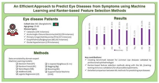
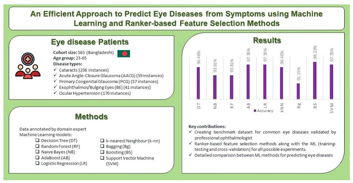
An Efficient Approach to Predict Eye Diseases from Symptoms Using Machine Learning and Ranker-Based Feature Selection Methods

1
Department of Computer Science, University of Calgary, Calgary, AB T2N 1N4, Canada
2
Department of Computer Science and Engineering, Daffodil International University, Dhaka 1341, Bangladesh
3
Department of Computer and Information Sciences, University of Delaware, Newark, DE 19716, USA
4
Department of Computer Engineering, Istanbul Medipol University, Istanbul 34810, Turkey
5
Department of Heath Informatics, University of Southern Denmark, 5230 Odense, Denmark
6
Ispahani Islamia Eye Hospital, Dhaka 1215, Bangladesh
*
Author to whom correspondence should be addressed.
Bioengineering 2023, 10(1), 25; https://doi.org/10.3390/bioengineering10010025
Submission received: 17 November 2022 / Revised: 13 December 2022 / Accepted: 19 December 2022 / Published: 24 December 2022

Abstract

:
The eye is generally considered to be the most important sensory organ of humans. Diseases and other degenerative conditions of the eye are therefore of great concern as they affect the function of this vital organ. With proper early diagnosis by experts and with optimal use of medicines and surgical techniques, these diseases or conditions can in many cases be either cured or greatly mitigated. Experts that perform the diagnosis are in high demand and their services are expensive, hence the appropriate identification of the cause of vision problems is either postponed or not done at all such that corrective measures are either not done or done too late. An efficient model to predict eye diseases using machine learning (ML) and ranker-based feature selection (r-FS) methods is therefore proposed which will aid in obtaining a correct diagnosis. The aim of this model is to automatically predict one or more of five common eye diseases namely, Cataracts (CT), Acute Angle-Closure Glaucoma (AACG), Primary Congenital Glaucoma (PCG), Exophthalmos or Bulging Eyes (BE) and Ocular Hypertension (OH). We have used efficient data collection methods, data annotations by professional ophthalmologists, applied five different feature selection methods, two types of data splitting techniques (train-test and stratified k-fold cross validation), and applied nine ML methods for the overall prediction approach. While applying ML methods, we have chosen suitable classic ML methods, such as Decision Tree (DT), Random Forest (RF), Naive Bayes (NB), AdaBoost (AB), Logistic Regression (LR), k-Nearest Neighbour (k-NN), Bagging (Bg), Boosting (BS) and Support Vector Machine (SVM). We have performed a symptomatic analysis of the prominent symptoms of each of the five eye diseases. The results of the analysis and comparison between methods are shown separately. While comparing the methods, we have adopted traditional performance indices, such as accuracy, precision, sensitivity, F1-Score, etc. Finally, SVM outperformed other models obtaining the highest accuracy of 99.11% for 10-fold cross-validation and LR obtained 98.58% for the split ratio of 80:20.

Graphical Abstract

1. Introduction

The eye is considered to be the most important sensory organ for humans and it plays a vital role in the overall ability of humans to interact with the world. Unfortunately many individuals in both rural and urban areas suffer from eye conditions such as cataracts, glaucoma, ocular hypertension, bulgy vision, etc. that affected their vision. There are a variety of causes for this such as age, diabetes, genetic and inheritance. Modern lifestyles, which have led to increased use of displays for digital devices, are also a factor affecting the vision.
These eye problems have a particularly high occurrence in many South Asian countries. As an example, in Bangladesh 1.5% of the adult population is blind and 21.6% of the population has low vision according to a survey presented in [1]. There are various reasons for this including the lack of vision care by individuals, pollution and excessive use of digital devices [1].
We chose individuals assumed to have one of the five eye diseases that are currently prevalent in Bangladesh and collected datafor the diseases (biomarkers and disease symptoms). These data are very important for any ophthalmologist or clinical professional since it is used to guide the treatment of the disease. It can also be used to train artificial intelligence algorithms that can ensure that the correct disease has indeed be diagnosed and provide automated recommendations for how to treat the disease.
From a literature search one finds that classic machine learning algorithms, especially classification algorithms, are the most appropriate for the detection and recommendation of the five eye diseases considered in this paper [2,3,4].
A dataset of eye-disorder-related data was compiled. This dataset will be used to make the eye disease classification easier and and it may also be used for further studies of eye diseases. Multiple machine learning techniques were applied to this dataset to test its applicability to the detection and classification tasks considered in this paper. The dataset can also be used to test other platforms such as Chabot, web apps, etc. which in turn can help the world with more accurate information about eye disease issues. One of the goals in this paper is also to make relevant and accurate medical information about eye diseases available to the medical community.
In the case of machine learning algorithms, it is also important that predictions can be explained since this provides insights into the predicted phenomena. Hence the explainable artificial intelligence (XAI) methods used here are of great help for the understanding of the eye disease symptoms for a given disease prediction.
The main contributions of this study are:
  • Creating a benchmark dataset in the domain of eye diseases validated by professional ophthalmologists, that cam be applied to test ML, AI and Symptomatic analyses.
  • Utilizing ranker-based feature selection methods to identify highly ranked symptoms among the five diseases.
  • Experimenting with scenarios both with and without splitting the dataset and with several feature selection methods for better predictions.
  • Compare the performance of classic ML methods to efficiently predict the occurrence of eye diseases.
For the remainder of the paper, Section 2 provides an overview of the five eye diseases that are considered in this study. Section 3 describes the existing related studies performed on these diseases. The proposed methodology along with detailed descriptions of each of the methodological steps are described in Section 4. The measurement indices used to measure the performance of the applied machine learning models are given in Section 5 and the experimental results are discussed in Section 6. A constructive discussion regarding the results and comparison of the model performances are presented in Section 7, and finally Section 8 concludes with suggestions for future improvements.

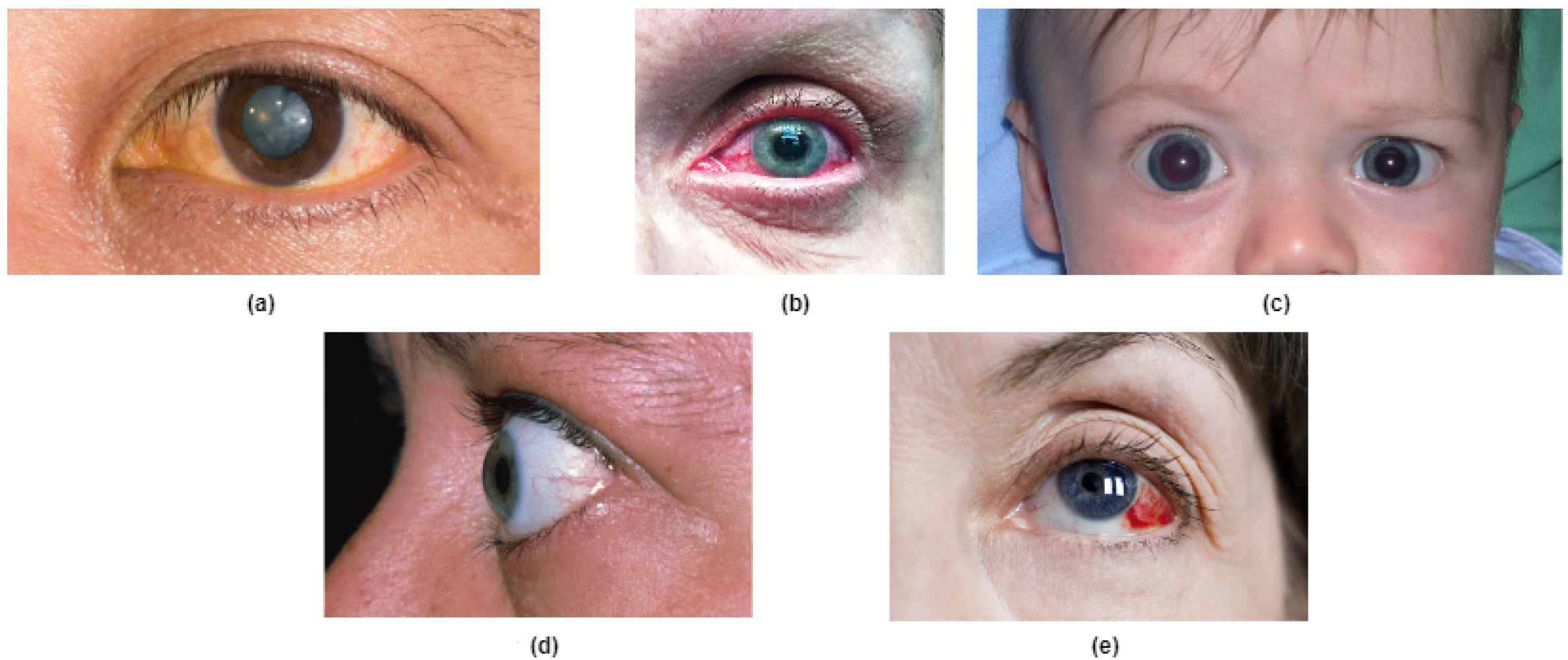
2. Overview of Five Eye Diseases

In this section, a brief overview of the five eye diseases that we have worked on is presented. For each disease, we describe the disease conditions, disease symptoms and disease risk factors. The images of the selected five categories of eye diseases are shown in Figure 1, however we have not used image data to identify or to annotate the dataset. Therefore, the sources or the images are referenced in the footnotes. The next five subsections describe the diseases worked on.

2.1. Cataracts

A dense and cloudy area that is usually formed on the lens of the eye is called a cataract. This cataract is an agglomeration of proteins situated in the eye that forms a lump-like mass which prevent the normal transmission of light through the lens to the retina. Some of the major symptoms appearing due to cataracts include degradation of night vision, blurry vision, faded colors and double vision. The different sub-types of cataracts are nuclear, cortical, posterior, congenital, senile, traumatic, bilateral as well as other subtypes. These sub-types are grouped into one disease category for this study to minimize the complexity of asociating the cataract with a specific sub-type. Smoking, older age, obesity, increased blood pressure, history of the same disease in family members, diabetes, exposure to radiation from X-ray and cancer treatments are the main risk factors associated with cataracts [5]. Cataracts are one of the common eye diseases in low and middle-income countries [6].

2.2. Acute Angle-Closure Glaucoma (AACG)

AACG is caused by a sudden increase in the intra-ocular pressure (IOP) which causes a displacement of the apposition of the iris to the trabecular meshwork. In acute angle-closure (AAC), the common symptoms are blurred vision, red eye, pain, headache, nausea and vomiting [7]. The process of AAC occurs suddenly with a dramatic onset of symptoms. Because of premorbid comorbidities, severely ill patients may encounter the risk of a sight-threatening condition. The drainage of the aqueous humor may be restricted causing high interior pressure that can result in critical damage to the optic nerve [7].

2.3. Primary Congenital Glaucoma (PCG)

PCG is another type of glaucoma caused by damage to the optic nerve [8]. High intra-ocular pressure in the eye is the main cause of the damage. It is identified when excessive tearing, light sensitivity, hazy cornea, redness of the eye, the closing of the eyelid and cloudy cornea symptoms are present. For this study, data for PGG patients are separated from the data for Secondary Congenital Glaucoma (SCG) patients. Having a previous related medical history in the family is considered one of the risk factors for PCG [9].

2.4. Exophthalmos or Bulging Eyes

Bulging eyes (BE) which is also known as exophthalmos, the medical term for BE. It is not a condition by itself, but a symptom of other conditions. Symptoms of BE include excessive dryness, visible whiteness, double vision and throbbing sensation in the eyes [10]. One or both eyes of a patient can be affected by BE and when it is present it may cause blinking problems.

2.5. Ocular Hypertension

Ocular hypertension (OH) is caused by poor drainage of the aqueous humor, the fluid inside the eye. Risk factors for developing OH are patients having a previous family history of ocular hypertension, glaucoma, diabetes, and age over 40. Patients having unbalanced diabetes or high blood pressure may be exposed to ocular hypertension [11].

3. Related Works

Papers relating to the prediction of eye diseases using artificial intelligence and machine learning are reviewed in this section since these areas discuss the tools that are used for the proposed method for efficiently predicting the five eye diseases discussed above. Some papers discussing explainable artificial intelligence methods are also included since some results from these paper are used for better interpretation of the results from the proposed method.
The few works that have been performed in the area of eye disease prediction using symptomatic data are also considered here.
One study assessed the prevalence of eye diseases in a certain low-income community in Bangladesh. The study was performed using in-person surveys and the results showed a higher prevalence of eye diseases than the world average. This reflects the difference in eye disease prevalence and diagnosis between individuals in low-income individuals and individuals with higher standards of living [1]. The study found that there is a funding and communication gap between vision related support for slum dwellers of Bangladesh and the Bangladesh community in general.
Ref. [12] is an epidemiology study of eye diseases that targets the Shahjadpur Children’s Cohort (SCC), a very interesting population-based cohort including only children with disabilities [12]. A chi-squared test, Fisher’s exact test and the binomial test were performed to find significant variations among the SCC. Sociodemographic details and the prevalence of childhood disabilities in the cohort study were included in the study.
Kadir et al. [13] performed a cross-sectional study of vision among 252 primary school-going children of the southern region of Bangladesh. The study was performed to assess the refractive errors (Myopia, Ametropia and Hyperopia) in the cohort and it was found that myopia is a common occurrence (50%).
We found some articles presenting methodologies to address eye disease classification using image processing techniques and ML algorithms. For these methodologies it is important for classification to have a large enough set of image data to run the models with image processing abilities that detect the region of interest (ROI) in the image. One article, Sakri et al. [14], presented an automated classification framework using image processing to classify diabetic eye disease (DED). Image enhancement techniques such as contrast limited adaptive histogram equalization (CLAHE), illumination correction and image segmentation techniques such as finding blood vessels, macular region and optic nerve were applied before applying the pre-trained model (VGG-16, Xception, ResNet50, CNN). All the models performed well with accuracies over 90% correct recognition. Similar image processing-based articles with different datasets can be found in [15,16,17,18].
Neural network based approach using the image dataset is a very common scenario in detecting eye diseases. Nazir et al. [19], extracted features using DenseNet-100 and applied improved CenterNet method on Aptos-2019 and IDrID dataset. The highest accuracy obtained in this method are 97.93% using the Aptos-2019 dataset and 98.10% using the IDrID dataset. The same dataset of Aptos-2019 has been used in [20], with feature fusion techniques and a deep neural network. The accuracy obtained in this method is 84.31%. Khan et al. [21] tried to manually extracted the retinal features with no feature-selection algorithms applied. The combination of CNN with VGG-19 has been proposed in this paper and accuracy obtained is 97.47%. Sarki et al. [22] and Pahuja et al. [23] also applied CNN for the image datasets and obtained accuracy less thatn 90% in both the case.
A data-driven approach for eye disease classification was adopted by Malik et al. [24]. The authors prepared a dataset having ten (10) attributes including age, gender and complaint (pain or blurred vision). Visual acuity of the right and left eye, pinhole value of the left and right eye, symptoms obtained from a slit lamp test (lids, upper lid, site, swelling), and posterior segment test are the overall symptoms considered in this study to determine the diagnosis glaucoma vs unspecified primary angle-closure glaucoma. NB (81.53%), DT (85.81%), Neural Network (86.98%) and RF (86.63%) models were applied to predict the diagnosis, and neural networks outperformed the other models.
A recent work [25] presented a multi-categorical common eye disease detection method using CNN. They prepared their own hand-crafted dataset which had 2250 images of cataracts, conjunctivitis and normal eyes. Three transfer learning models (VGG-16, Resnet-50 and Inception-v3) were applied, where the class-wise performance evaluation was shown for each model. Inception-v3 (97.08%) outperformed VGG-16 (95.48%) and Resnet-50 (95.78%) in the experiments and they claimed the results to be the highest among the other image-based eye disease classification approaches [26,27,28,29].
From the review of the existing works, we found a gap in finding the most relevant symptoms for different types of eye diseases as well as the lack of a benchmark dataset with symptomatic data of eye diseases. In this study, we have focused on these gaps and we have designed a research methodology to fill the gaps.

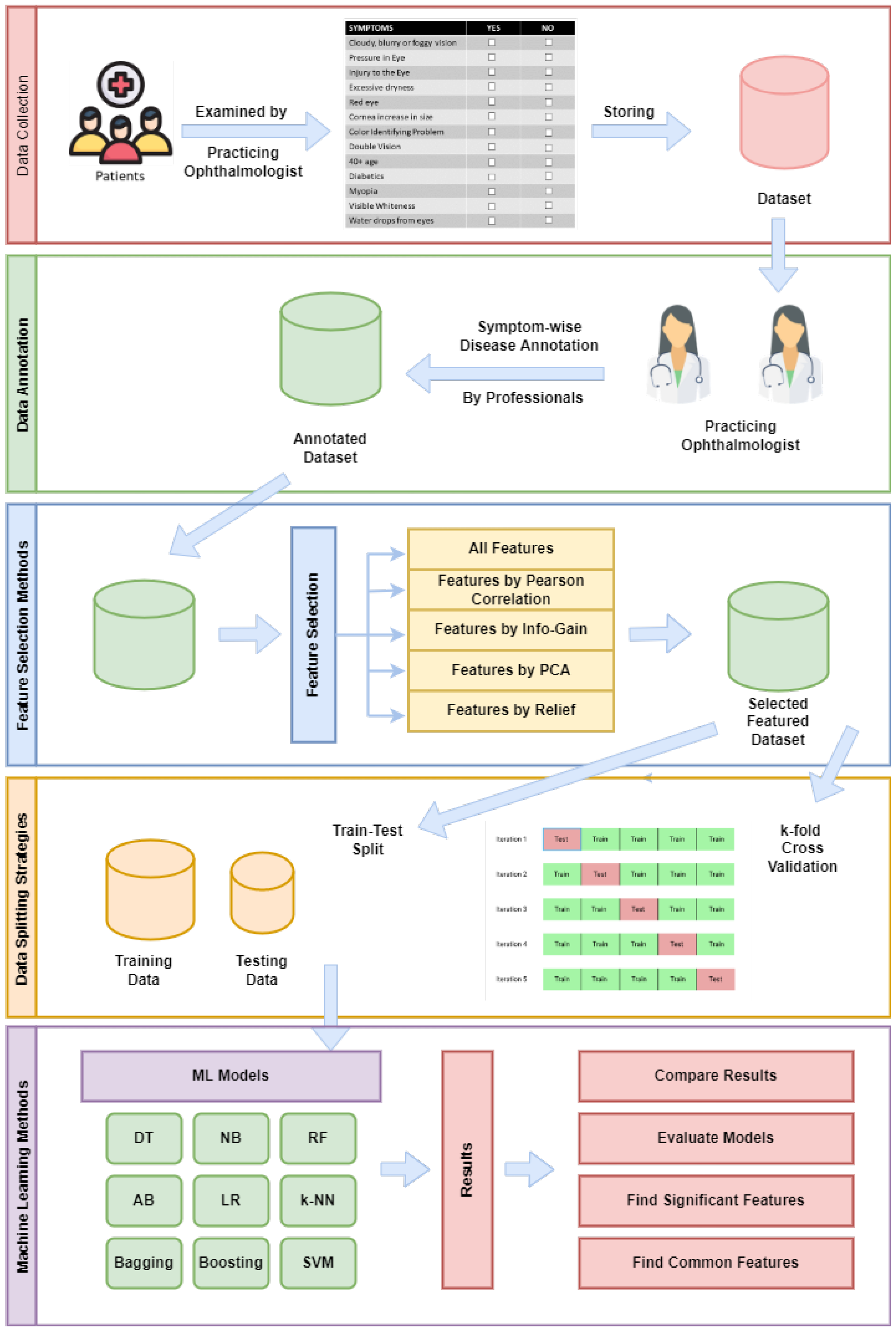
4. Research Methodology

An overview of the research methodology adopted for eye disease predictions in this study is shown diagrammatically in Figure 2. The steps of the process are highlighted, starting from the data collection from patients to the application of ML and XAI methods. The remainder of this section elaborates on the steps of the proposed methodology.

4.1. Data Collection

Data collection processes have in general to be executed rigorously in order to create a valid and useful dataset. The data collected has to include both symptoms and biomarker data for each patient included in the dataset. For this study, we have included real-world patients data collected when they were present during a referral to an ophthalmologist. Since it can be very difficult to track the symptoms by the ophthalmologist during a short visit, there were two interviewers (ophthalmologist and one of the author) collecting the data. The statistical properties of the dataset acquired are presented in Table 1.
The patients were examined by a practicing ophthalmologist while checking the conditions and biomarkers listed in Table 2 for each of the patients. The dataset collected contains 563 patients data having any one of the eye diseases mentioned in Section 2. The data collection was also conducted in a closed-room environment during one-to-one appointments and the attributes noted in Table 2 were collected. A value, either 0 or 1 has been assigned for each attributes based on the observation of the ophthalmologist to avoid a missing value in the dataset. This makes it a robust dataset having no missing values.

4.2. Data Annotation

Data annotation or labeling of the dataset used for the training of a methodology that is based on supervised machine learning algorithms is the most critical and important step in the development of the methodology. If the annotation or labeling of the data is not performed properly then the acceptability of the whole methodology might be questioned. In this case, the data collection was performed very carefully. While collecting the data, the ophthalmologist played the role of an interviewer and the patients played the role of an interviewee. Questions associated with the 19 attributes were asked and properly examined by the ophthalmologist to determine the right kind of eye disease that the patient had. Hence, the ophthalmologist worked as the annotator of the dataset. Therefore, the dataset created for the study has been validated by domain experts, hence it can be considered as a benchmark dataset in this domain. Each attribute is labeled either zero (0) or one (1) based on the examination performed by the ophthalmologist. The annotated dataset contains 19 attributes/symptoms and one (1) class label indicating the eye disease. This annotated dataset was forwarded to the next step in the feature selection process.

4.3. Feature Selection Methods

For the feature selection step, we considered ranker-based feature selection methods, so that we got a list of attributes, in this case, symptoms. It is expected that this selected symptom list may be significant for predicting a particular eye disease more efficiently.
The ranker-based methods utilized in this study are Pearson Correlation (PC), Information Gain (IG), Principal Component Analysis (PCA), Relief-based Ranking (RR) and all features. The methods were applied directly to the annotated data and the ranking scores of each attribute were determined. Brief descriptions of the feature selection methods are given next.
The Pearson Correlation (PC)-based feature selection [30] method is widely used in machine learning problems. The ( ρ X , Y ) is calculated using Equation (1) where c o v ( X , Y ) is the covariance between the X and Y and σ the standard deviations (SDs) on the X and Y:
ρ X , Y = c o v ( X , Y ) σ X σ Y
The X and Y can be considered as class-feature or feature-feature relationships. X can be the class and Y can be the feature or X can be the feature and Y can be another feature. The ρ X , Y value is between the −1 and +1, where −1 means a negative correlation between X and Y where 0 means no correlation between X and Y and +1 means a positive correlation between X and Y. The higher the ρ X , Y -value the higher the correlation between X and Y is. Therefore, for our study, we have chosen the class-feature relationship. We calculated the class-feature correlation values for all the features and ranked them by the correlation values from high to low. Depending on the ranking, we selected some of the features to run further steps of the ML models.
Information Gain (IG) is another widely accepted feature selection method for various research problems for example where text categorization is used [31,32]. This is evidenced by the use of IG in several research domains, such as computer vision [32] and text classification [33]. IG is a ratio value calculated by Equation (2).
I G ( T , a ) = H ( T ) v v a l u e s ( a ) | x T | x a = v | | T | · H ( x T | x a = v )
Here, v a l u e s ( a ) is the set of all possible values of features a A t t r where A t t r is the set of all features, H is the entropy, and x T denotes the value of specific example x for a A t t r . The largest I G is the smallest entropy.
Principal Component Analysis (PCA) was invented by Karl Pearson, see [34,35], initially as an analog of the principal axis theorem in mechanics. After the development of eigenvalue decomposition and other related theorems, the use of PCA became more popular. PCA is the method for calculating the principal components of a dataset. This multivariate technique tries to analyze the data in which the observations are kept by several inter-correlated quantitative variables, which are dependent [36]. PCA can be used as a method to reduce the dimension of the data to handle high dimension data for a given process [37]. The dimensionality reduction is performed by choosing an optimal number of eigenvectors to account for some percentage of variance in the original data.
Relief is a filter-based feature selection algorithm presented by Kira and Rendell in 1992 [38]. The algorithm takes a data set with p instances of n number of features. The method iterated m times starting with a n-long weight vector W. In each iteration the weight vector is updated as in Equation (3).
W i = W i ( x i n e a r H i t i ) 2 + ( x i n e a r M i s s i ) 2
For each iteration, the feature vector (X) is assigned to one random instance, and the closest same-class instance is called ‘near-hit’. Similarly, the closest different-class instance is called ‘near-miss’. Therefore, the weight of any given attribute will decrease if it differs from that feature and increase in the reverse case.
An associated ranker method ranking the features by their individual evaluators (Correlation, GainRatio, Components and Relief) was implemented with the feature selection methods. The method may choose a specific number of features to be retained for the remainder of the process. We have kept the default value ( 1 ) to find the ranking over all the features. No initial set of features was chosen to bias the whole process. Therefore, all of the features are considered as initial inputs to the methods.

4.4. Data Splitting Strategies

For the ML algorithms, especially when applying classifiers, it is very important to perform data splitting for the train-test mechanism [39]. One part of the data is used for training the models and the rest of the data are used for testing the performance of the model. Therefore, the choice of what percentage should be used for training and what percentage should be used for testing can be critical. In this study, we adopted two data-splitting strategies: Train-Test and k-fold Cross Validation.
For the Train(%)-Test(%) technique, we split the data using 66–34%, 75–25% and 80–20%. Using the different splits we ran the same models on the data, to find the performance of the ML algorithm.
The second data splitting strategy is k-fold Cross Validation [40]. Though it is a kind of sampling method, it has been found to be effective in the area of ML while doing the Train–Test split. In a single fold of cross-validation, the data are partitioned into two parts (training and testing) and in the second fold, the same data are partitioned randomly. In this paper, k-fold was used, which means that the original data sample was randomly partitioned into k equal-sized sub-samples. Among those k sub-samples, one sub-sample was considered for testing and the rest of the sub-samples were considered for training and the same process was run k-times. In the same manner, as for the Train-Test strategy, we chose 3-fold, 5-fold and 10-fold Cross Validation for finding the best-performing ML algorithm.

4.5. Machine Learning Methods

The naive Bayes classifier simplifies the classifying process considerably by assuming that the presence of a particular feature in a class is not related to any other feature in the class [41]. Although this independence is generally a poor assumption, in practice naive Bayes often competes well with more sophisticated classifiers [41]. Our broad goal was to understand the data characteristics which affect the performance of naive Bayes [41]. Our approach used Monte Carlo simulations that allow a systematic study of classification accuracy for several classes of randomly generated problems [41]. The success of naive Bayes in the presence of feature dependencies can be explained as follows: optimality in terms of zero-one loss (classification error) is not necessarily related to the quality of the fit to a probability distribution (i.e., the appropriateness of the independence assumption). Rather, an optimal classifier is obtained as long as both the actual and estimated distributions agree on the most probable class [41]. For example, naive Bayes optimality can be proven for some problem classes that have a high degree of feature dependencies, such as disjunctive and conjunctive concepts [41].
The k Nearest Neighbor (k-NN) method is a popular classification method in data mining and statistics because of its simple implementation and excellent classification performance [42]. However, it is impractical for traditional k-NN methods to assign a fixed k value (even if it is set by experts) to all test samples [42]. Previous solutions assigned different k values to different test samples by the cross-validation method but this was usually time-consuming [42]. This paper proposes a k-Tree method to learn different optimal k values for different test/new samples, by involving a training stage in the k-NN classification [42].
For a simplified description, decision tree analysis is a divide-and-conquer approach to classification (and regression which is not covered within the scope of this review) [43]. Decision trees can be used to discover features and extract patterns in large databases that are important for discrimination and predictive modeling [43]. These characteristics, coupled with their intuitive interpretation, have been some of the reasons for the extensive use of decision trees for both exploratory data analysis and predictive modeling applications for more than two decades [43]. Decision trees have an established foundation in both the machine learning and artificial intelligence literature and a niche in the use of decision trees in both the chemical and biochemical sciences is slowly developing [43].
In the same manner, as contingency table analyses and two tests, Logistic Regression (LG) allows the analysis of dichotomous or binary outcomes with two mutually exclusive levels and it allows the use of continuous or categorical predictors and provides the means for adjusting for multiple predictors [44]. This makes LG especially useful for the analysis of observational data when adjustments are needed to reduce the potential bias resulting from differences in the groups being compared [44].

5. Performance Measurement Indices

We adapted the widely accepted measurement tools accuracy, precision, recall and F1-score for evaluating the performance of the applied ML methods. Usage of these measurement indices can be found in many existing works, including [45,46]. While calculating these indices, the positive or negative classification of the diseases is taken into account. The following Equations (4)–(7) were used for generating the measurements.
A c c u r a c y ( A C C ) = T P + T N T P + T N + F P + F N
P r e c i s i o n = T P T P + F P
S e n s i t i v i t y ( S E N ) = T P T P + F N
F 1 s c o r e = 2 ( P r e c i s i o n × R e c a l l ) ( P r e c i s i o n + R e c a l l )
Here, T P is True Positive (when the ML model correctly classifies a patient as having a particular eye disease), T N is True Negative (when the ML model correctly classifies a patient as having a different eye disease), F P is False Positive (when the ML model incorrectly classifies a patient as having one particular disease when the patient actually has another disease) and F N is False Negative (when the Ml model incorrectly classifies a patient as not having a disease when the patient actually has the disease).

6. Experimental Results

In this section, we show the detailed results of the experiments. After applying the feature selection methods the selected features along with their ranking values are given in this section. The experiments were executed based on splitting and feature selection. The performance measurement indices mentioned in Section 5 were used to describe the outcomes of the experiments.

6.1. Applying Feature Selection Methods

We applied multiple ranker-based feature selection techniques and the ranking score of the features is therefore important when choosing the high-scored features for the further process. The ranking score, attribute names and numbers are shown for PC, IG and RR in Table 3, Table 4 and Table 5, respectively. PCA on the other hand gives a ranking with associated attributes for obtaining the best results based on the outcome or class. Therefore, it only ranked the first sixteen (16) features, as shown in Table 6. After applying the FS methods, the first ten attributes were selected and considered for the next steps.

6.2. Experiments on Data Splitting and FS Methods

We devised four (4) experiments to test multiple data-splitting strategies and feature selection techniques. All of the ML methods were applied in these experiments. For the first two experiments, we considered splitting with and without the feature selection applied. For the next two experiments, cross-validation was applied with and without feature selection methods. As described in Section 4, subsection D, 66–34%, 75–25% and 80–20% are the splitting criteria used and 3-fold, 5-fold and 10-fold cross-validations are applied.

6.2.1. Experiment-1: Splitting + FS Applied

Data splitting was performed and five feature selections were applied for this experiment. The effect of the selection features can be found in this experiment. Comparison of precision and recall/sensitivity values are shown in Figure 3.
The accuracy values for each of the models for different train-test split scenarios are shown in Figure 4 and Figure 5. The highest accuracy obtained for XGBoost is 98.23%.

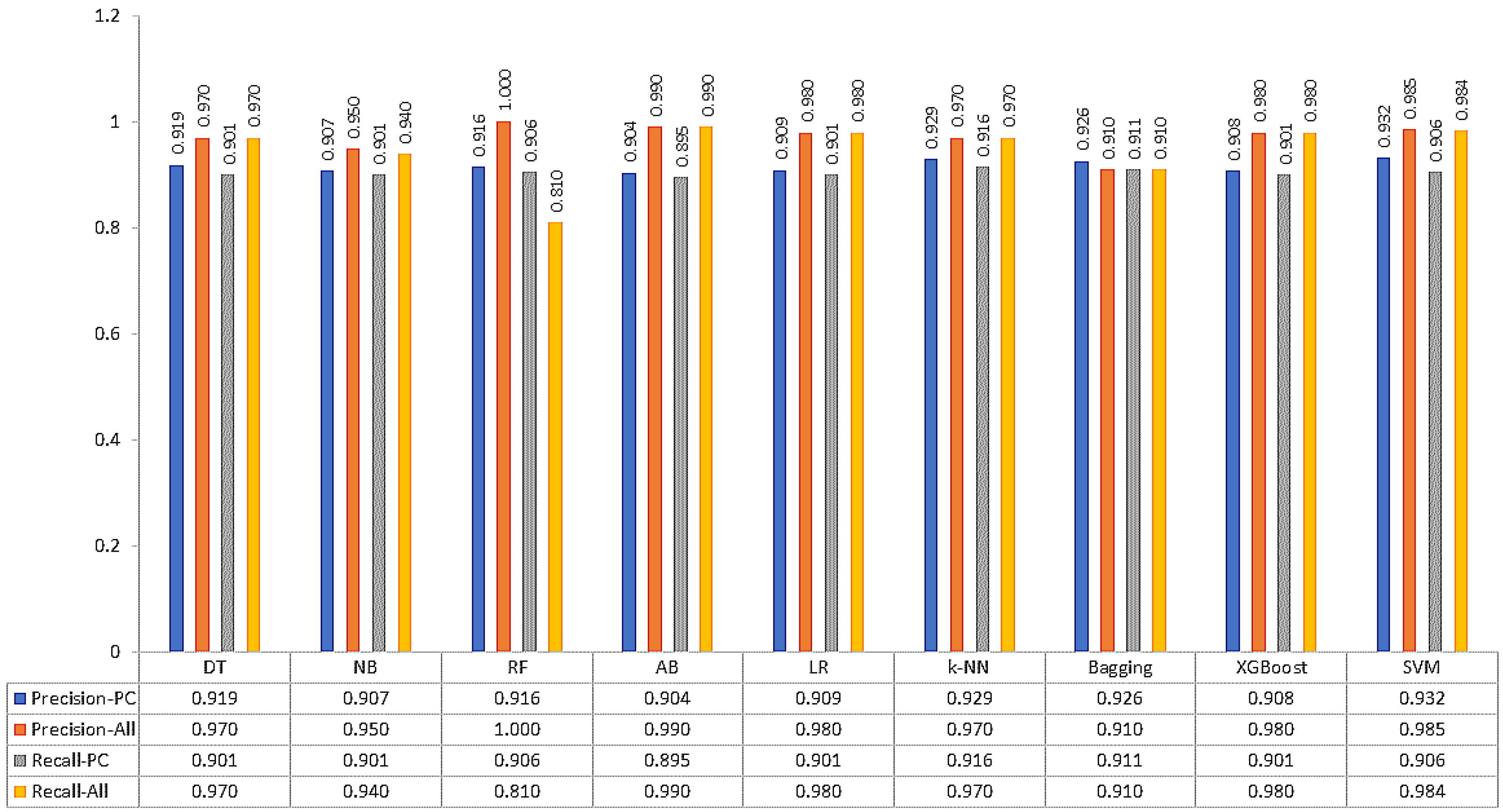
6.2.2. Experiment-2: Splitting + No FS Applied

For experiment-2, splitting was applied, but the FS methods were not applied. Precision, recall, F1-score and accuracy of the ML models are shown in Table 6. XGBoost performs better overall showing more than 98% accuracy for all types of splits. The highest accuracy reported was 98.582% when LR was used in a 75–25% split.

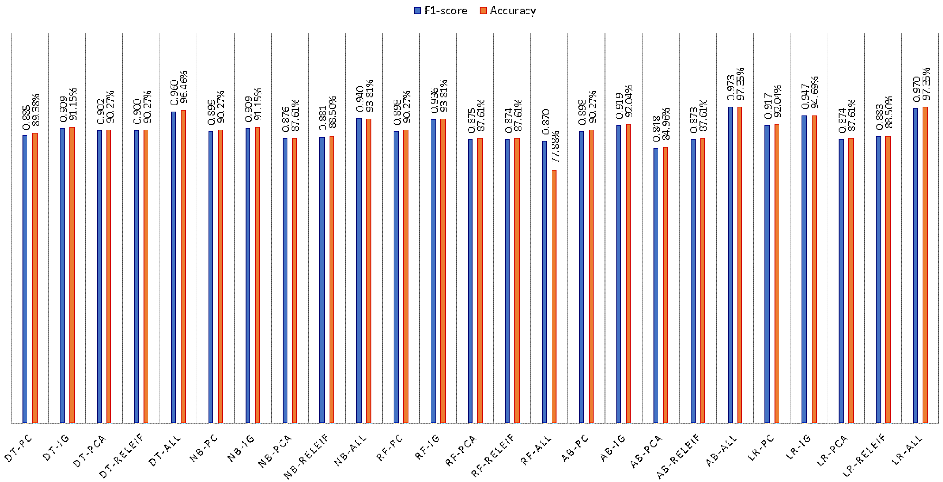
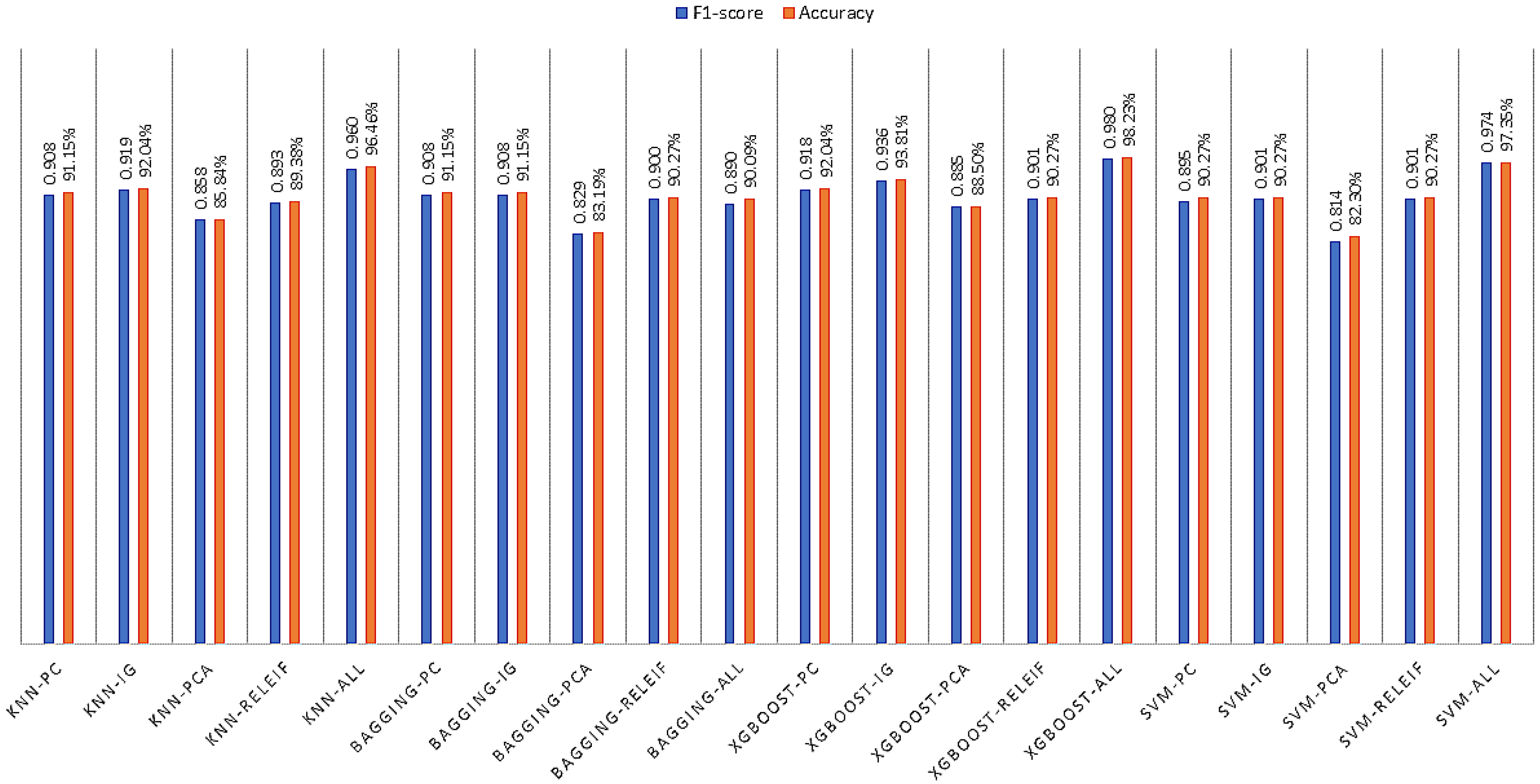
6.2.3. Experiment-3: Cross-Validation + FS Applied

In experiment-3, we applied a cross-validation technique instead of a split with the application of five feature selection strategies. This resulted in a total of one hundred and thirty-five (135) runs of the ML models with different setups. This rigorous experiment gave us the most suitable ML model among all the models chosen for the study. The precision, recall, F1-score and accuracy values are presented in Table 7. Among all the models, LR outperformed other models showing 98.94% accuracy.

6.2.4. Experiment-4: Cross-Validation + No FS Applied

In experiment-4, we applied three different cross-validation methods, but this time without selecting any particular features coming from the FS methods. This method can be easily compared to experiment-2 to compare the percentage split and cross-validation methods. Table 8 shows the precision, sensitivity, F1-score and accuracy values for each of the ML models. SVM showed the highest accuracy of 99.11% in this experimental setup. Table 9 shows the same measurements as Table 8 for cross-validation without the FS methods. And SVM outperforms the other algorithms in 10-fold cross-validation obtaining 99.110% accuracy.

7. Discussion

7.1. Finding Significant Features

The list of significant features based on the feature selection algorithms is depicted in Table 3, Table 4, Table 5 and Table 6. The selected features or attributes can be considered better choices among the other symptoms of eye disease. The first ten selected features can be formulated as four different feature sets outputted from PC-based ( F P C ), IG-based ( F I G ), PCA-based ( F P C A ), and Relief-based ( F R e l i e f ) feature selection methods, as below.
F P C = < a 1 , a 2 , a 3 , a 5 , a 7 , a 8 , a 9 , a 11 , a 12 , a 15 >
F I G = < a 1 , a 2 , a 3 , a 7 , a 8 , a 9 , a 11 , a 12 , a 13 , a 15 >
F P C A = < a 1 , a 2 , a 3 , a 4 , a 10 , a 13 , a 14 , a 16 , a 17 , a 18 >
F R e l i e f = < a 1 , a 2 , a 3 , a 7 , a 8 , a 9 , a 11 , a 12 , a 15 , a 18 >

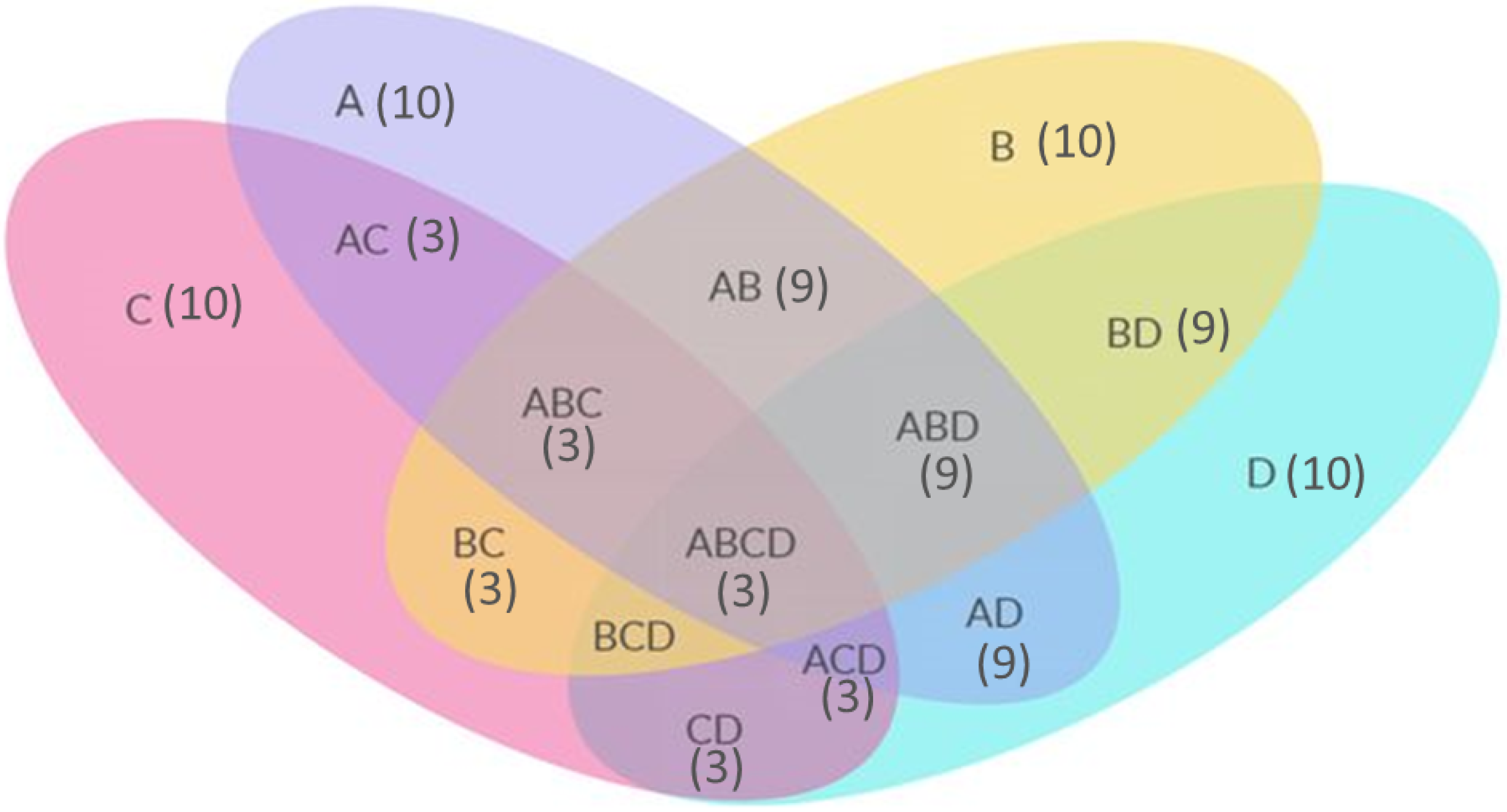
7.2. Finding Common Features

Considering the selected feature sets in Equations (8)–(11), the common set can be found calculating the intersection of the features.
F P C F I G = < a 1 , a 2 , a 3 , a 7 , a 8 , a 9 , a 11 , a 12 , a 13 >
F P C F P C A = < a 1 , a 2 , a 3 >
F P C F R e l i e f = < a 1 , a 2 , a 3 , a 7 , a 8 , a 9 , a 11 , a 12 , a 13 >
F I G F P C A = < a 1 , a 2 , a 3 , a 13 >
F I G F R e l i e f = < a 1 , a 2 , a 3 , a 7 , a 8 , a 9 , a 11 , a 12 , a 13 >
F P C A F R e l i e f = < a 1 , a 2 , a 3 >
F P C F I G F P C A F R e l i e f = < a 1 , a 2 , a 3 >
Considering F P C as A, F I G as B, F P C A as C and F R e l i e f as D, the Venn diagram in Figure 6 shows the common features among the sets. The numbers inside the elipses shows the number of features they have in common. For example, AB (9) means there are 3 common features between A and B. Similarly, ABCD (3) means there are 3 common features between the A, B, C, and D sets.

7.3. Comparison with Existing Works

In this section, we have compared our proposed work with the existing works on the same domain focusing on the prediction of eye disease. Most of the works from literature, used image data to detect eye disease. The images contain the disease region of interest (RoI) and it is easier to identify the RoI by the experienced ophthalmologists. The challenge of annotation can be handled easily by the domain experts and then the supervised learning algorithms would be appropriate for the prediction. The recent advancements of machine learning and deep learning methods also encouraged the researchers to exploit them for the eye disease detection. The following Table 10 shows the comparison with the recent existing works from the literature with our proposed approach. None of the approaches mentioned in Table 10 have applied feature selection algorithms to find out the significant symptom features. We have applied several feature selection methods to find out the significant and common features affecting the organ. Our proposed approach obtained highest accuracy 99.11% (SVM) by exploring the classical ML methods.

8. Conclusions

This paper presents an efficient approach for predicting five different eye diseases and shows a comparative analysis among the ML methods for predicting the five common eye diseases from a benchmark dataset. The most critical issue with suitable dataset for ML models is annotation or class labelling. For our work, we have annotated the data by practicing ophthalmologist, which gives more accurate and validate data for the models. Therefore, the ML models are showing very satisfactory results in terms of accuracy values, as most of then showing accuracy above 90% and all the models are showing accuracy over 70%. The highest accuracy obtained is 99.11% from SVM with cross-validation and without applying any feature selection methods. The significant features are identified using feature selection methods and the intersection of the selected features are showing the common features. From the common features we obtain the understanding of the symptoms responsible for the eye diseases. One of the shortcomings of the paper is that we have not used any images for the predictive analysis. Using image data along with the annotated symptom data would have provide better solution to a multi-model approach. In future works, a multivariate or uni-variate analysis may be conducted to identify specific symptoms and acquire insights about a particular eye disease. The application of explainable artificial intelligence to interpret the best model could be another improvement of this work.

Author Contributions

Conceptualization, A.A.M. and M.M.M.; methodology, A.A.M. and M.M.M.; software, A.A.M.; validation, A.A.M., M.M.M., J.R. and R.A.; formal analysis, A.A.M. and M.M.M.; investigation, A.A.M., M.M.M. and O.J.; resources, A.A.M. and O.J.; data collection, A.A.M. and O.J.; data curation, A.A.M. and O.J.; writing—original draft preparation, A.A.M. and M.M.M.; writing—review and editing, A.A.M., J.R. and R.A.; visualization, A.A.M. and M.M.M.; supervision, R.A. and J.R.; project administration, A.A.M., M.M.M., R.A. and J.R. All authors have read and agreed to the published version of the manuscript.

Funding

This research received no external funding.

Institutional Review Board Statement

The study was conducted in accordance with the Faculty of Graduate Studies of Daffodil International University and approved by the Institutional Review Board (or Research Ethics Committee of Faculty of Science and Information Technology) (Application No: REC-FSIT-20220816001, 08/16/2022).

Informed Consent Statement

Informed consent was obtained from all patients involved in the study.

Data Availability Statement

Data are available from the corresponding author and can be shared with anyone upon reasonable request.

Conflicts of Interest

The authors declare no conflict of interest.

References

  1. Sutradhar, I.; Gayen, P.; Hasan, M.; Gupta, R.D.; Roy, T.; Sarker, M. Eye diseases: The neglected health condition among urban slum population of Dhaka, Bangladesh. BMC Ophthalmol. 2019, 19, 38. [Google Scholar] [CrossRef] [Green Version]
  2. Ayodele, T.O. Types of machine learning algorithms. New Adv. Mach. Learn. 2010, 3, 19–48. [Google Scholar]
  3. Mair, C.; Kadoda, G.; Lefley, M.; Phalp, K.; Schofield, C.; Shepperd, M.; Webster, S. An investigation of machine learning based prediction systems. J. Syst. Softw. 2000, 53, 23–29. [Google Scholar] [CrossRef] [Green Version]
  4. Mackenzie, A. The production of prediction: What does machine learning want? Eur. J. Cult. Stud. 2015, 18, 429–445. [Google Scholar] [CrossRef] [Green Version]
  5. Hodge, W.G.; Whitcher, J.P.; Satariano, W. Risk factors for age-related cataracts. Epidemiol. Rev. 1995, 17, 336–346. [Google Scholar] [CrossRef]
  6. Liu, Y.-C.; Wilkins, M.; Kim, T.; Malyugin, B.; Mehta, J.S. Cataracts. The Lancet 2017, 390, 600–612. [Google Scholar] [CrossRef]
  7. Petsas, A.; Chapman, G.; Stewart, R. Acute angle closure glaucoma—A potential blind spot in critical care. J. Intensive Care Soc. 2017, 18, 244–246. [Google Scholar] [CrossRef] [Green Version]
  8. Ko, F.; Papadopoulos, M.; Khaw, P.T. Primary congenital glaucoma. Prog. Brain Res. 2015, 221, 177–189. [Google Scholar] [PubMed]
  9. Badawi, A.H.; Al-Muhaylib, A.A.; Al Owaifeer, A.M.; Al-Essa, R.S.; Al-Shahwan, S.A. Primary congenital glaucoma: An updated review. Saudi J. Ophthalmol. 2019, 33, 382–388. [Google Scholar] [CrossRef]
  10. Moro, A.; Munhoz, R.P.; Arruda, W.O.; Raskin, S.; Teive, H.A.G. Clinical relevance of “bulging eyes” for the differential diagnosis of spinocerebellar ataxias. Arquivos de Neuro-Psiquiatria 2013, 71, 428–430. [Google Scholar] [CrossRef] [Green Version]
  11. Argus, W.A. Ocular hypertension and central corneal thickness. Ophthalmology 1995, 102, 1810–1812. [Google Scholar] [CrossRef] [PubMed]
  12. Muhit, M.; Karim, T.; Jahan, I.; Al Imam, M.H.; Das, M.C.; Khandaker, G. Epidemiology of eye diseases among children with disability in rural Bangladesh: A population-based cohort study. Dev. Med. Child Neurol. 2022, 64, 209–219. [Google Scholar] [CrossRef]
  13. Kadir, S.M.U.; Ali, M.; Islam, M.S.; Parvin, R.; Quadir, A.S.M.; Raihani, M.J.; Islam, A.R.; Ahmmed, S. Prevalence of Refractive Errors among Primary School Children in the Southern Region of Bangladesh. Community Based Med. J. 2022, 11, 41–45. [Google Scholar] [CrossRef]
  14. Sarki, R.; Ahmed, K.; Wang, H.; Zhang, Y.; Ma, J.; Wang, K. Image preprocessing in classification and identification of diabetic eye diseases. Data Sci. Eng. 2021, 6, 455–471. [Google Scholar] [CrossRef]
  15. Umesh, L.; Mrunalini, M.; Shinde, S. Review of image processing and machine learning techniques for eye disease detection and classification. Int. Res. J. Eng. Technol. 2016, 3, 547–551. [Google Scholar]
  16. Oda, M.; Yamaguchi, T.; Fukuoka, H.; Ueno, Y.; Mori, K. Automated eye disease classification method from anterior eye image using anatomical structure focused image classification technique. In Proceedings of the Medical Imaging 2020: Computer-Aided Diagnosis, Houston, TX, USA, 16–19 February 2020; Volume 11314, pp. 991–996. [Google Scholar]
  17. Fourcade, A.; Khonsari, R.H. Deep learning in medical image analysis: A third eye for doctors. J. Stomatol. Oral Maxillofac. Surg. 2019, 120, 279–288. [Google Scholar] [CrossRef]
  18. Acharya, U.R.; Kannathal, N.; Ng, E.Y.K.; Min, L.C.; Suri, J.S. Computer-based classification of eye diseases. In Proceedings of the 2006 International Conference of the IEEE Engineering in Medicine and Biology Society, New York, NY, USA, 30 August–3 September 2006; pp. 6121–6124. [Google Scholar]
  19. Nazir, T.; Nawaz, M.; Rashid, J.; Mahum, R.; Masood, M.; Mehmood, A.; Hussain, A. Detection of diabetic eye disease from retinal images using a deep learning based CenterNet model. Sensors 2021, 21, 5283. [Google Scholar] [CrossRef]
  20. Bodapati, J.D.; Shaik, N.S.; Naralasetti, V. Deep convolution feature aggregation: An application to diabetic retinopathy severity level prediction. Signal Image Video Process. 2021, 15, 923–930. [Google Scholar] [CrossRef]
  21. Khan, M.S.M.; Ahmed, M.; Rasel, R.Z.; Khan, M.M. Cataract detection using convolutional neural network with VGG-19 model. In Proceedings of the 2021 IEEE World AI IoT Congress (AIIoT), Seattle, WA, USA, 10–13 May 2021; pp. 0209–0212. [Google Scholar]
  22. Sarki, R.; Ahmed, K.; Wang, H.; Zhang, Y.; Wang, K. Convolutional neural network for multi-class classification of diabetic eye disease. EAI Endorsed Trans. Scalable Inf. Syst. 2022, 9, e15. [Google Scholar] [CrossRef]
  23. Pahuja, R.; Sisodia, U.; Tiwari, A.; Sharma, S.; Nagrath, P. A Dynamic Approach of Eye Disease Classification Using Deep Learning and Machine Learning Model. In Proceedings of Data Analytics and Management; Springer: Singapore, 2022; pp. 719–736. [Google Scholar]
  24. Malik, S.; Kanwal, N.; Asghar, M.N.; Sadiq, M.A.A.; Karamat, I.; Fleury, M. Data driven approach for eye disease classification with machine learning. Appl. Sci. 2019, 9, 2789. [Google Scholar] [CrossRef] [Green Version]
  25. Bitto, A.K.; Mahmud, I. Multi categorical of common eye disease detect using convolutional neural network: A transfer learning approach. Bull. Electr. Eng. Inform. 2022, 11, 2378–2387. [Google Scholar] [CrossRef]
  26. Verma, S.; Singh, L.; Chaudhry, M. Classifying red and healthy eyes using deep learning. Illumination 2019, 10, 525–531. [Google Scholar] [CrossRef]
  27. Hameed, S.; Ahmed, H.M. Eye diseases classification using back propagation with parabola learning rate. Al-Qadisiyah J. Pure Sci. 2021, 26, 1–9. [Google Scholar] [CrossRef]
  28. Bhadra, A.A.; Jain, M.; Shidnal, S.S. Automated detection of eye diseases. In Proceedings of the 2016 International Conference on Wireless Communications, Signal Processing and Networking (WiSPNET), Chennai, India, 23–25 March 2016; pp. 1341–1345. [Google Scholar] [CrossRef]
  29. Prasad, K.; Sajith, P.S.; Neema, M.; Madhu, L.; Priya, P.N. Multiple eye disease detection using Deep Neural Network. In Proceedings of the TENCON 2019—2019 IEEE Region 10 Conference (TENCON), Kochi, India, 17–20 October 2019; pp. 2148–2153. [Google Scholar] [CrossRef]
  30. Pearson, K. On the Criterion That a Given System of Deviations From the Probable in the Case of a Correlated System of Variables is Such That It Can Be Reasonably Supposed to Have Arisen From Random Sampling. Philos. Mag. 1900, 5, 157–175. [Google Scholar] [CrossRef] [Green Version]
  31. Forman, G. An extensive empirical study of feature selection metrics for text classification. J. Mach. Learn. Res. 2003, 3, 1289–1305. [Google Scholar]
  32. Gao, Z.; Xu, Y.; Meng, F.; Qi, F.; Lin, L. Improved information gain-based feature selection for text categorization. In Proceedings of the 2014 4th International Conference on Wireless Communications, Vehicular Technology, Information Theory and Aerospace & Electronic Systems (VITAE), Aalborg, Denmark, 11–14 May 2014; pp. 11–14. [Google Scholar]
  33. Yu, L.; Liu, H. Feature selection for high-dimensional data: A fast correlation-based filter solution. In Proceedings of the 20th International Conference on Machine Learning (ICML-03), Washington, DC, USA, 21–24 August 2003; pp. 856–863. [Google Scholar]
  34. Pearson, K. LIII. On lines and planes of closest fit to systems of points in space. Lond. Edinb. Dublin Philos. Mag. J. Sci. 1901, 2, 559–572. [Google Scholar] [CrossRef] [Green Version]
  35. Available online: https://en.wikipedia.org/wiki/Principal_component_analysis (accessed on 18 December 2022).
  36. Abdi, H.; Williams, L.J. Principal component analysis. Wiley Interdiscip. Rev. Comput. Stat. 2010, 2, 433–459. [Google Scholar] [CrossRef]
  37. Song, F.; Guo, Z.; Mei, D. Feature selection using principal component analysis. In Proceedings of the 2010 International Conference on System Science, Engineering Design and Manufacturing Informatization, Yichang, China, 12–14 November 2010; pp. 27–30. [Google Scholar]
  38. Kira, K.; Rendell, L.A. The feature selection problem: Traditional methods and a new algorithm. AAAI 1992, 2, 129–134. [Google Scholar]
  39. Abraham, M.T.; Satyam, N.; Lokesh, R.; Pradhan, B.; Alamri, A. Factors affecting landslide susceptibility mapping: Assessing the influence of different machine learning approaches, sampling strategies and data splitting. Land 2021, 10, 989. [Google Scholar] [CrossRef]
  40. Refaeilzadeh, P.; Tang, L.; Liu, H. Cross-validation. Encycl. Database Syst. 2009, 5, 532–538. [Google Scholar]
  41. Rish, I. An empirical study of the Naive Bayes classifier. In Proceedings of the JCAI 2001 Workshop on Empirical Methods in Artificial Intelligence, Seattle, DC, USA, 4–6 August 2001; Volume3, pp. 41–46. [Google Scholar]
  42. Zhang, S.; Li, X.; Zong, M.; Zhu, X.; Wang, R. Efficient kNN classification with different numbers of nearest neighbors. IEEE Trans. Neural Netw. Learn. Syst. 2017, 29, 1774–1785. [Google Scholar] [CrossRef] [PubMed]
  43. Myles, A.J.; Feudale, R.N.; Liu, Y.; Woody, N.A.; Brown, S.D. An introduction to decision tree modeling. J. Chemom. J. Chemom. Soc. 2004, 18, 275–285. [Google Scholar] [CrossRef]
  44. LaValley, M.P. Logistic regression. Circulation 2008, 117, 2395–2399. [Google Scholar] [CrossRef]
  45. Marouf, A.A.; Hasan, M.K.; Mahmud, H. Comparative analysis of feature selection algorithms for computational personality prediction from social media. IEEE Trans. Comput. Soc. Syst. 2020, 7, 587–599. [Google Scholar] [CrossRef]
  46. Ghosh, P.; Azam, S.; Jonkman, M.; Karim, A.; Shamrat, F.J.M.; Ignatious, E.; Shultana, S.; Beeravolu, A.R.; De Boer, F. Efficient prediction of cardiovascular disease using machine learning algorithms with relief and LASSO feature selection techniques. IEEE Access 2021, 9, 19304–19326. [Google Scholar] [CrossRef]
Figure 1. Typical images of eye diseases. (a) Cataracts, (b) Acute angle-closure glaucoma, (c) Primary congenital glaucoma, (d) Exophthalmos or bulging eyes, and (e) Ocular hypertension.
Bioengineering 10 00025 g001
Figure 2. Overview of working diagram of the proposed eye disease prediction method.
Bioengineering 10 00025 g002
Figure 3. Precision and Recall values of ML methods with 66–34% split and PC-based FS method.
Bioengineering 10 00025 g003
Figure 4. F1-score and Accuracy values of DT, NB, RF, AB and LR with 80%–20% split and five FS method.
Bioengineering 10 00025 g004
Figure 5. F1-score and Accuracy values of k-NN, Bagging, XGBoost and SVM with 80–20% split and five FS method.
Bioengineering 10 00025 g005
Figure 6. Venn Diagram showing the common features among the feature sets.
Bioengineering 10 00025 g006
Table 1. Statistical Properties of Dataset.
PropertiesAmount/Values
No. of patients563
Age group of patients23–65
Gender of patientsMale or Female
No. of instances in the dataset563
Data collection processIn-person interview with patients
Type of interviewSemi-structured interviews
Type of pre-defined questionnaireBinary closed questions (Yes/No)
Types of eye diseases
  • Cataracts (236 instances)
  • Acute Angle-Closure Glaucoma (AACG) (59 instances)
  • Primary Congenital Glaucoma (PCG) (57 instances)
  • Exophthalmos/Bulging Eyes (BE) (41 instances)
  • Ocular Hypertension (170 instances)
Table 2. Attributes used for data collection.
No.AttributesProperties
a1Cloudy, blurry or foggy visionThe values are either 0 or 1
a2Pressure in eye
a3Injury to the eye
a4Excessive dryness
a5Red eye
a6Cornea increased in size
a7Problem in identifying color
a8Double vision
a9Myopia
a10Trouble with glasses
a11Hard to see in the dark
a12Visible whiteness
a13Mass pain
a14Vomiting
a15Water drops from eyes continuously
a16Presence of light when eye lid closes
a17Family history of similar disease
a18Age +40Biomarker (0 or 1)
a19Diabetes
Table 3. Ranking of Features and associated correlation coefficient values from PC-based FS method.
Ranking ScoreAttributes (Attribute Number)
0.6218Cloudy, blurry or foggy vision (a1)
0.5583Problem in identifying color (a7)
0.5340Double vision (a8)
0.5148Water drops from eyes continuously (a15)
0.5114Pressure in eye (a2)
0.5073Hard to see in the dark (a11)
0.4991Myopia (a9)
0.3052Injury to the eye (a3)
0.2403Mass pain (a13),
0.2279Red eye (a5)
0.2258Vomiting (a14)
0.2225Cornea increased in size (a6)
0.2225Presents of light when eyelid close (a16)
0.2061Visible whiteness (a12)
0.2023Excessive dryness (a4)
0.153940+ Age (a18)
0.1531Family history of similar disease (a17)
0.1525Diabetes (a19)
0.0524Trouble with glasses (a10)
Table 4. Ranking of Features from Information Gain-based FS method.
Ranking ScoreAttributes (Attribute Number)
0.8000Cloudy, blurry or foggy vision (a1)
0.6182Problem in identifying color (a7)
0.5587Water drops from eyes continuously (a15)
0.5434Double vision (a8)
0.5430Pressure in eye (a2)
0.5216Myopia (a9)
0.4848Hard to see in the dark (a11)
0.3477Injury to the eye (a3)
0.2326Mass pain (a13)
0.2293Visible whiteness (a12)
0.2196Excessive dryness (a4)
0.2130Cornea increased in size (a6)
0.2130Presents of light when eyelid close (a16)
0.2108Red eye (a5)
0.2004Vomiting (a14)
0.074940+ Age (a18)
0.0730Family history of similar disease (a17)
0.0718Diabetes (a19)
0.0000Trouble with glasses (a10)
Table 5. Ranking of Features from Relief-based FS method.
Ranking ScoreAttributes (Attribute Number)
0.6194Cloudy, blurry or foggy vision (a1)
0.4196Pressure in eye (a2)
0.4181Problem in identifying color (a7)
0.3682Injury to the eye (a3)
0.3383Myopia (a9)
0.3253Double vision (a8)
0.3186Water drops from eyes continuously (a15)
0.3137Hard to see in the dark (a11)
0.112940+ Age (a18)
0.1032Visible whiteness (a12)
0.1024Red eye (a5)
0.1013Cornea increased in size (a6)
0.0952Diabetes (a19)
0.0915Mass pain (a13)
0.0875Excessive dryness (a4)
0.0826Vomiting (a14)
0.0773Presents of light when eyelid close (a16)
0.0616Family history of similar disease (a17)
0.0218Trouble with glasses (a10)
Table 6. Ranking of Features from PCA-based FS method.
Ranking ScoreAttributes (Attribute Number)
0.7619Cloudy, blurry or foggy vision (a1)
0.5981Injury to the eye (a3)
0.5054Excessive dryness (a4)
0.4171Presents of light when eyelid close (a16)
0.365Trouble with glasses (a10)
0.3175Pressure in eye (a2)
0.271940+ Age (a18)
0.2306Family history of similar disease (a17)
0.1976Vomiting (a14)
0.1678Mass pain (a13)
0.1389Red eye (a5)
0.1136Double vision (a8)
0.09Cornea increased in size (a6)
0.0719Problem in identifying color (a7)
0.0549Myopia (a9)
0.0388Hard to see in the dark (a11)
Table 7. Performance of ML models in experiment-2 (Splitting + No FS Applied).
Model66–34% Split75–25% Split80–20% Split
NamePRSENF1-ScoreACCPRSENF1-ScoreACCPRSENF1-ScoreACC
DT0.970.970.9796.875%0.970.970.9797.163%0.970.960.9696.460%
NB0.950.940.9494.271%0.960.950.9595.035%0.950.940.9493.805%
RF1.000.810.8881.25%1.000.820.8981.56%1.000.780.8777.876%
AB0.980.980.9897.51%0.980.980.9898.05%0.980.980.9897.69%
LR0.980.980.9897.917%0.990.990.9998.582%0.970.970.9797.345%
k-NN0.970.970.9796.875%0.970.970.9797.163%0.960.960.9696.46%
Bagging0.910.910.9191.513%0.910.840.8291.56%0.800.900.8990.088%
XGBoost0.980.980.9898.579%0.990.990.9998.581%0.980.980.9898.23%
SVM0.640.740.6574.479%0.630.740.6473.759%0.590.700.5969.912%
Table 8. Performance of ML models in experiment-3 (Cross Validation + FS Applied).
Cross Fold Validation with FS Method
MethodsFeature Selection Methods3-fold5-fold10-fold
PRF1ACCPRF1ACCPRF1ACC
DTPC0.9140.8920.89289.17%0.9180.8990.90089.88%0.9130.8970.89689.70%
IG0.9020.8930.89689.34%0.9060.8970.89989.70%0.9070.8990.89989.88%
PCA0.9250.9110.91291.12%0.9260.9130.91491.30%0.9260.9130.91491.30%
Relief0.9160.8990.89989.88%0.9210.8990.89989.88%0.9180.8990.89989.88%
All *0.9600.9500.95094.85%0.9600.9600.96096.81%0.9300.9300.92096.98%
NBPC0.9200.9090.90790.94%0.9230.9090.90790.94%0.9220.9090.90790.94%
IG0.9240.9150.91391.47%0.9100.9090.90990.94%0.8980.8990.89889.88%
PCA0.9240.9110.91391.12%0.9250.9110.91391.12%0.9260.9110.91391.12%
Relief0.9160.9040.90290.41%0.9120.9010.89990.05%0.9160.9020.90190.23%
All *0.9600.9600.96095.56%0.9600.9600.95095.92%0.9500.9300.39095.74%
RFPC0.9200.9060.90590.59%0.9230.9110.91091.12%0.9190.9080.90790.76%
IG0.9080.9020.90190.23%0.9230.9150.91591.47%0.9180.9090.90990.94%
PCA0.9110.8990.90189.88%0.8950.8900.89088.99%0.8990.8920.89389.17%
Relief0.9230.9040.90290.41%0.9240.9040.90490.41%0.9230.9040.90390.41%
All *0.9900.9900.99098.40%1.0001.0001.00098.58%1.0001.0001.00097.87%
ABPC0.9130.9010.90090.05%0.9230.9080.90890.80%0.9210.9080.90790.76%
IG0.9110.9020.90190.23%0.9130.9040.90590.41%0.9250.9130.91391.30%
PCA0.8950.8900.89088.99%0.9090.9010.90190.05%0.9050.8970.89889.70%
Relief0.9200.9020.90190.23%0.9260.9090.90890.94%0.9200.9040.90390.41%
All *0.9750.9750.97597.51%0.9800.9800.98098.05%0.9770.9770.97797.69%
LRPC0.9190.9020.90490.23%0.9240.9110.91191.12%0.9220.9090.90990.94%
IG0.9210.9090.91090.94%0.9130.9080.90890.76%0.9270.9170.91791.65%
PCA0.9000.8930.89589.34%0.9040.8990.90089.88%0.9110.9020.90490.23%
Relief0.9270.9110.91291.12%0.9260.9090.90990.94%0.9300.9130.91391.30%
All *0.9900.9800.95098.58%1.0001.0001.00098.94%1.0001.0001.00098.94%
k-NNPC0.9300.9150.91391.47%0.9290.9170.91591.65%0.9260.9150.91291.47%
IG0.9080.9080.90790.76%0.9120.9060.90790.59%0.9260.9150.91591.47%
PCA0.8920.8860.88788.63%0.9060.8990.89989.88%0.9010.8950.89689.52%
Relief0.9290.9080.90890.76%0.9250.9060.90690.59%0.9220.9020.90290.23%
All *0.9600.9600.95096.45%0.9800.9700.97096.27%1.0001.0001.00096.63%
BaggingPC0.9140.8970.89689.70%0.9260.9090.90790.94%0.9250.9110.91091.00%
IG0.9090.8920.88989.17%0.8980.8970.89489.70%0.8970.8950.89389.30%
PCA0.9110.8990.89989.88%0.9090.8950.89589.52%0.9050.8900.88988.99%
Relief0.9050.8850.88588.45%0.9110.8970.89389.70%0.9140.8970.89689.70%
All *0.9300.9400.97095.06%0.9400.9600.95095.58%0.9400.9500.89095.58%
XGBoostPC0.9200.9040.90590.41%0.9260.9110.91291.12%0.9260.9110.91191.12%
IG0.9290.9170.91791.65%0.9200.9110.91391.12%0.9240.9130.91591.30%
PCA0.9160.9060.90790.59%0.9150.9060.90790.59%0.9180.9080.90990.76%
Relief0.9290.9130.91391.30%0.9230.9080.90890.76%0.9270.9090.91090.94%
All *0.9800.9800.98098.58%0.9900.9900.99098.58%0.9800.9800.98098.05%
SVMPC0.9340.9110.90791.12%0.9350.9130.90791.30%0.9280.9110.90591.12%
IG0.9170.9090.91190.94%0.9130.9060.90790.59%0.8980.8900.89188.99%
PCA0.9040.8880.88888.81%0.9020.8900.88888.99%0.8990.8920.89189.17%
Relief0.9350.9110.90991.12%0.9320.9080.90690.76%0.9310.9080.90690.76%
All *0.9800.9800.98098.76%1.0001.0001.00098.94%1.0001.0001.00099.11%
* All features, P: Precision, R: Recall, F1: F1-score, ACC: Accuracy.
Table 9. Performance of ML models in experiment-4 (Cross-validation + No FS Applied).
Model3-fold5-fold10-fold
NamePRSENF1-ScoreACCPRSENF1-ScoreACCPRSENF1-ScoreACC
DT0.960.950.9594.850%0.960.960.9696.805%0.930.930.9296.980%
NB0.960.960.9695.561%0.960.960.9595.915%0.950.930.9395.742%
RF0.990.990.9998.402%1.001.001.0098.581%1.001.001.0097.870%
AB0.980.980.9897.510%0.980.980.9898.050%0.980.980.9897.690%
LR0.990.980.9598.579%1.001.001.0098.936%1.001.001.0098.938%
k-NN0.960.960.9596.447%0.980.970.9796.271%1.001.001.0096.626%
Bagging0.930.940.9795.062%0.940.960.9595.579%0.940.950.8995.578%
XGBoost0.980.980.9898.579%0.990.990.9998.581%0.980.980.9898.051%
SVM0.980.980.9898.756%1.001.001.0098.936%1.001.001.0099.110%
Table 10. Comparison with existing works.
Existing WorksFeatures UsedFeature Selection UsedMethodsEvaluation
Nazir et al. [19]Extracted features using Densenet-100NoImproved CenterNetAccuracy (using Aptos-2019 dataset: 97.93%, using IDrID dataset: 98.10%)
Bodapati et al. [20]Feature fusionNoDeep neural NetworkAccuracy (using Aptos-2019 dataset: 84.31%)
Khan et al. [21]Manual extracted retinal featuresNoCNN with VGG-19Accuracy (97.47%)
Sarki et al. [22]NoneNoCNN with RMSprop OptmizerAccuracy (81.33%)
Pahuja et al. [23]NoneNoSVM and CNNAccuracy (SVM:87.5% and CNN: 85.42%)
Malik et al. [24]NoneNoDT, NB, RF and NNAccuracy (RF: 86.63%)
ProposedNoneYes (PC, IG, PCA, Relief)DT, NB, RF, AB, LR, k-NN, Bagging, XGBoost and SVMAccuracy (Highest Accuracy Obtained: 99.11% (SVM))
Disclaimer/Publisher’s Note: The statements, opinions and data contained in all publications are solely those of the individual author(s) and contributor(s) and not of MDPI and/or the editor(s). MDPI and/or the editor(s) disclaim responsibility for any injury to people or property resulting from any ideas, methods, instructions or products referred to in the content.

