Remote Sensing of Sediment Discharge in Rivers Using Sentinel-2 Images and Machine-Learning Algorithms

Abstract

The spatio-temporal dynamism of sediment discharge (Q_s) in rivers is influenced by various natural and anthropogenic factors. Unfortunately, most rivers are only monitored at a limited number of stations or not gauged at all. Therefore, this study aims to provide a remote-sensing-based alternative for Q_s monitoring. The at-a-station hydraulic geometry (AHG) power–law method was compared to the at-many-stations hydraulic geometry (AMHG) method; in addition, a novel AHG machine-learning (ML) method was introduced to estimate water discharge at three gauging stations in the Tisza (Szeged and Algyő) and Maros (Makó) Rivers in Hungary. The surface reflectance of Sentinel-2 images was correlated to in situ suspended sediment concentration (SSC) by support vector machine (SVM), random forest (RF), artificial neural network (ANN), and combined algorithms. The best performing water discharge and SSC models were employed to estimate the Q_s. Our novel AHG ML method gave the best estimations of water discharge (Szeged: R² = 0.87; Algyő: R² = 0.75; Makó: R² = 0.61). Furthermore, the RF (R² = 0.9) and combined models (R² = 0.82) showed the best SSC estimations for the Maros and Tisza Rivers. The highest Q_s were detected during floods; however, there is usually a clockwise hysteresis between the SSC and water discharge, especially in the Tisza River.

1. Introduction

Sediment is a substance that has been eroded from rocks by physical and chemical processes and is moved by gravity, water, wind, or by their combination. The term “fluvial sediment” refers to the sediment transported by rivers [1]. Fluvial sediment has many benefits, as it controls the global carbon cycle, morphological evolution of river channels, and delta development. Furthermore, it improves the agricultural productivity of the floodplain soils due to the deposition of nutrient-rich material [2]. In natural systems, climate and tectonics are the main driving factors of continental erosion [3] and thus of fluvial sediment availability [4]. However, the various anthropogenic activities (e.g., land use/land cover changes, construction of dams, mining activities, runoff, and erosion control) and climate change alter the quantity and timing of the fluvial sediment formation and transport. For instance, Martinez et al. [5] studied the sediment discharge of the Amazon River between 1995 and 2007, and the findings revealed that the suspended sediment concentrations rose by 20% due to changes in land use/land cover and global rainfall patterns. On the other hand, others [6,7] reported a considerable decrease in the sediment discharge of the Yellow and Mississippi Rivers due to the construction of sediment trapping systems and soil conservation activities.

Quantifying the amount of transported sediment in rivers plays an important role in various engineering works. For example, reservoirs should be designed to be large enough to accommodate the expected deposited sediment throughout their lifetimes, or the drop of sediment discharge downstream of reservoirs has to be predicted to protect the hydraulic structures downstream from clear water erosion (the phenomenon occurs downstream of the trapping structures due to losing a significant amount of suspended and bedload; thus, water begins to erode once more). Furthermore, any changes in sediment discharge quantities could lead to environmental problems. For example, the increased sediment released into coastal waters might destroy the marine ecosystem, whereas the decreased discharge could result in delta shoreline retreat [8]. In addition, the suspended sediment can contain not only natural particles but also solid pollutants, such as microplastics [9]. Therefore, sediment discharge monitoring is a critical issue not only in hydrology and geomorphology but also in water quality studies and in the protection of the entire ecological system. As there are various types of sediment transport (e.g., suspended and bedload), there are different methods to quantify them. In the present study, the focus is on suspended sediment transport of medium-sized rivers (Tisza and Maros in Hungary); therefore, we will focus on the suspended load of rivers in the rest of the Introduction. The most common way of suspended sediment discharge quantification is to measure the discharge at a given cross-section of the river and the corresponding suspended sediment concentration.

The water discharge of a river is directly related to the meteorological runoff (precipitation–evaporation) and catchment area [10]; thus, rivers with high runoff and limited catchment area could produce discharges as large as rivers with low runoff and extended catchment area. Land use/land cover changes, urban growth, and climate change could also have an impact on water discharge and its long-term variability [11]. The rating curve principle introduced by Leopold and Maddock [12] is being used to estimate discharge in a wide range of rivers around the globe. This method considers a power–law relationship between the flow width (w), average depth (d) and average velocity (v), and discharge (Q). These rating curves could be calibrated and validated by several in situ methods that can be used to measure discharge, such as current meter and acoustic doppler current profiler (ADCP) [13]. Despite the usefulness of the rating method, the fitted curves should be revised continuously (particularly in mobile-bed streams) to avoid inaccuracies caused by the morphological evolution of channels. The sand-bedded channels could change even during one flood wave due to the significant amount of scouring and fill, which leads to hysteresis (looping) of the rating curves [14,15]. For instance, the same discharge (3500 m³/s) was reported at two separate stages (rising stage: 885 cm; falling stage: 930 cm) during the 1970 flood in the Tisza River (at Szeged, Hungary) due to the hysteresis of the rating curve [14]. In the longer term, the natural evolution of the channels could be influenced by various engineering works, e.g., river damming, cut-offs, construction of artificial levees, revetments, and groynes, which influence the channel development for decades or centuries [14,16,17,18]. Thus, the rating curves have to be revisited and verified from time to time.

The greatest problem with in situ discharge measurements is that they are very labor intensive; therefore, discharge data are spatially and temporally limited. As a result, many rivers and river sections around the world remain ungauged, and those that have been gauged are seeing a dramatic fall in the number of stations owing to budget deficit [2,19,20]. Therefore, more research attention has focused on discharge acquisition using remote-sensing methods, especially with the great development of the spatial, spectral, and temporal resolution of the earth observation systems (e.g., Landsat, Sentinel-2, Worldview, Spot) and their synoptic coverage [21]. River discharge was estimated by combining remote-sensing data with either hydrological models [22,23,24,25,26] or hydraulic models [27,28,29,30]; however, these methods require the availability of many ancillary ground-based data. Thus, researchers have exploited the Leopold and Maddock [12] theory to estimate discharge from one hydraulic parameter (e.g., width or stage or slope) [2,19,31,32,33,34,35,36,37,38,39].

Kouraev et al. [39] and Birkinshaw et al. [36] utilized the TOPEX/Poseidon and ENVISAT/ERS-2 altimetry data, respectively, to obtain water stage and discharge by rating curves. Similarly, Michailovsky et al. [37] employed Envisat altimetry data to obtain water stages over the Zambezi River basin, which were then translated into discharges using three different methods (e.g., rating curves, synchronous in situ measurement of cross-section and discharge, and the available historical data of discharge), with RMSE ranges between 4.1% and 13.8%. The river width is considered the most obvious hydraulic parameter that can be observed from space. Gleason and Smith [31] estimated river discharge at mass conserved reaches along many rivers by width measurements obtained from satellite images and at-a-station hydraulic geometry (AHG; Leopold and Maddock [12]). However, they discovered a log-linear relationship between the AHG coefficients and exponents of the cross-sections along mass conserved reaches of rivers, which is called at-many-stations hydraulic geometry (AMHG). In addition, if these coefficients and exponents are optimized to minimize the discharge difference between every pair of cross-sections, better discharge estimations will be obtained. Therefore, they estimated the reach discharge based on optimized AHG coefficients and exponents of several cross-sections. Durga Rao et al. [35] estimated the discharge of four Indian rivers at different discharge conditions using a time series of width data obtained by Landsat and IRS satellite images and the AMHG approach. The AMHG coefficients and exponents were optimized by a genetic algorithm, and the results showed good accuracies, especially during low and medium stages. Comparably, Mengen et al. [32] followed a similar approach to estimate the discharge of the Mekong River, utilizing Sentinel-1 data (active sensor) to obtain river width instead of passive sensor data.

In order to calculate or measure the suspended sediment discharge of a river, the sediment characteristics and its transport rate should also be known. The suspended sediment usually has a size range between 0.45 µm and 2000 µm [40]. In general, the bedload forms 5–20% of the total sediment transport of rivers [40], whereas the rest forms the suspended load and wash load. However, this percentage range is quite rough, as, in lowland rivers with abundant suspended sediment supply, the proportion of bedload could be less than 1% [41]. The suspended sediment concentration in rivers can be estimated by collecting water samples manually or automatically (e.g., passive samplers, automated pumping, or time-integrating samplers). The manual method can be implemented under the depth integrated approach, by collecting samples from the whole depth [42,43], or under the point integrated approach, when a sample is collected from a single point at the water surface [44]. Despite the great accuracy of the in situ methods for measuring suspended sediment concentration, they are very time consuming and labor intensive; moreover, their results are just limited to the given sampling station. As a result, many studies investigated the suspended sediment concentrations in rivers using remote-sensing images, exploiting the ability of suspended sediment to increase reflectance values at visible and near-infrared spectra [45,46,47,48,49,50]. The correlation between suspended sediment concentration and reflectance of satellite images was performed by semi-empirical approach [46,51,52], bio-optical modeling approach [53,54], or machine-learning algorithms [55,56,57].

Few studies attempted to retrieve sediment discharge using the remote-sensing method [2,3,5,58,59,60]. Some of them estimated sediment discharge by combining in situ measurement of discharge and remotely sensed suspended sediment concentration [5,58,59,60]; others used satellite gravimetry data to estimate sediment discharge of large rivers [3]; and fewer obtained both water discharge and suspended sediment concentration from satellite images to compute sediment discharge [2].

In Hungary, the medium-sized Tisza and Maros Rivers transport a large amount of suspended sediment (Tisza: 18.7 million t/y; Maros: 8.3 million t/y). The dominance of suspended sediment in their sediment budget is well reflected by the low proportion of their bedload transport (Tisza: 0.04%; Maros: 0.3%). Unfortunately, only 8 sediment gauging stations operate on the 962 km long Tisza and only one on the 750 km long Maros (Figure 1). In addition, the measurements are performed just once a month, regardless of the water stage. However, more frequent spatial and temporal data are needed to support environmental studies of the river system. Therefore, this study aims to calibrate and validate suspended sediment and discharge models for the Tisza and Maros Rivers by in situ and Sentinel-2 data. The derived models could be employed to estimate sediment discharge at ungauged periods. The detailed goals of this study are to: (1) derive the river discharge models based on AHG and AMHG methods, in addition to assessing the applicability and stability of discharge models derived by combing AHG with machine-learning algorithms, which was not assessed in the literature; (2) calibrate the suspended sediment models based on machine-learning algorithms, such as artificial neural network (ANN), support vector machine (SVM), and random forest (RF), comparing their results and performance; (3) apply the best derived suspended sediment and discharge models to historical images of Sentinel-2 (ungauged periods) to produce a longer time series of sediment discharge of both rivers within the study area.

2. Materials and Methods

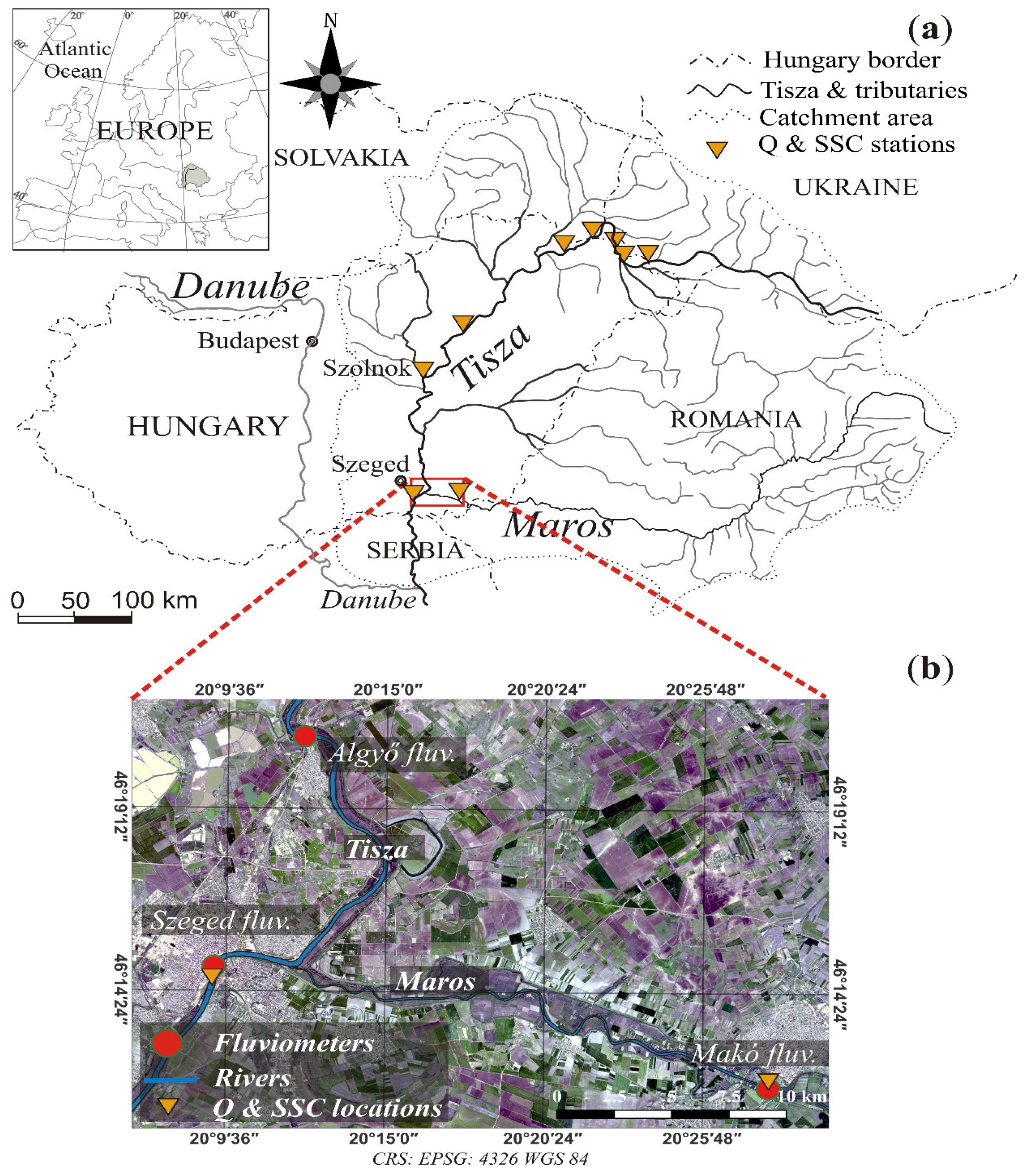
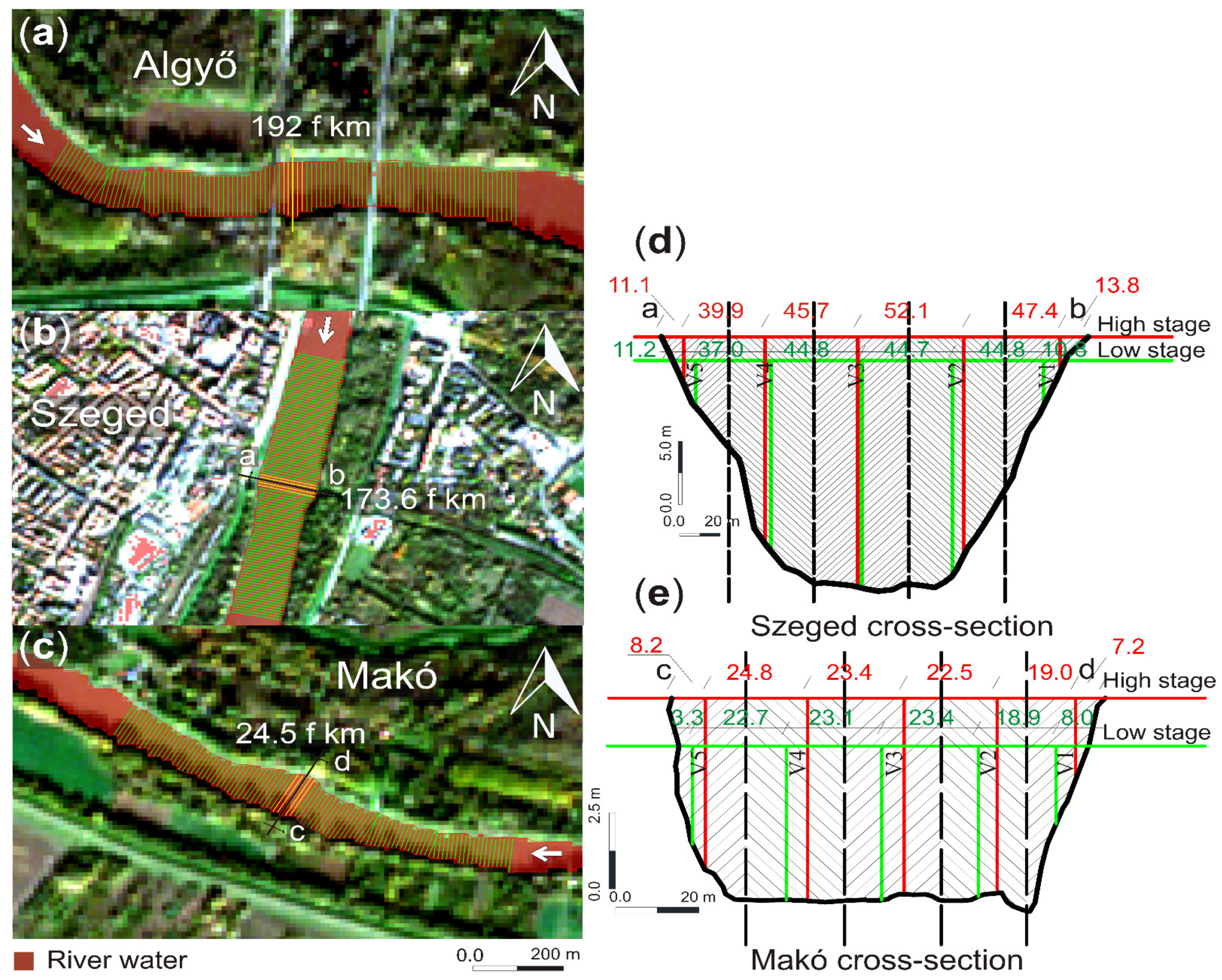
2.1. Study Area

The presented research studied the suspended sediment transport of the Tisza and Maros Rivers in the eastern part of the Carpathian Basin, central Europe. The Tisza River is the longest tributary (962 km) of the Danube [16], and its catchment area (157,200 km²) covers 19.5% of the Danube’s catchment area [61]. The Maros/Mures River is the greatest tributary of the Tisza (length: 750 km; catchment area: 30,000 km²) and one of the most dynamic rivers of the Carpathian Basin [62]. The study was performed at their confluence area (Figure 1). The Maros joins the Tisza at 177 fluvial km (f km) of the Tisza, with a confluence angle of 23° [47]. The Lower Tisza is wider (164 m on average) and considerably deeper (14.1 m) than the Lower Maros (width: 126 m; depth: 4.26 m; [18,63]).

The flood of the Maros usually precedes the flood of the Tisza by a few days; however, they could also occur simultaneously during long-lasting floods [64]. As a result of their low slope conditions, they could be impounded by the Danube or each other [47,62]. Usually both rivers have a flood period in early spring (March–April) caused by snowmelt and in early summer (June–July) due to summer rainfall. Usually, the early spring flood conveys more discharge (15% of the annual transported water [65] and sediment) than the early summer flood [16,62]. Sometimes the summer flood superimposes the spring flood (e.g., in 2006) because of the low slope (2.9 cm/km; [16,66]) on the long lowland section of the Tisza River, which results in high flood waves [62]. The floods of the Tisza usually cover the floodplain for 2–3 months; however, they extend for only 1–2 weeks in the Maros River due to its greater slope (Lower Maros: 28 cm/km; [16,66]).

The mean discharge of the Lower Tisza is ca. six times that of the Maros (Tisza at Szeged: 930 m³/s; Maros at Makó: 161 m³/s). On the other hand, the mean water velocities of both rivers are very close (Maros: 0.66 m/s; Tisza: 0.54 m/s; [16]). There is a huge difference between the lowest and highest stages, which is 13.55 m on the Tisza and 7.28 m for the Maros [16].

Both rivers transport a substantial amount of suspended sediment. Based on in situ measurements (1970–2000), the Lower Tisza’s mean annual suspended sediment load is 18.7 million t/y, and its mean concentration is 640 g/m³. However, in the confluence area with the Maros, the sediment conditions change considerably [67], as the Maros transports 8.3 million t/y suspended sediment (mean concentration: 1600 g/m³) into the Tisza [16,47,68].

There are considerable spatio-temporal variations in the amount of transported suspended sediment along the Tisza River (Figure 2). The main reasons for the spatial variations between two subsequent gauging stations are the aggradation of suspended sediment in the channel during low stages, which can be mobilized by small flood waves, and sedimentation on the floodplain [69]. The suspended sediment budget is probably also influenced by deposition in reservoirs and bank erosion, though they were not evaluated. According to the measurements on the Middle Tisza, at Szolnok and Kisköre [69,70], the suspended sediment concentration rapidly grows during the rising limb of the flood waves, and it reaches its maximum before the peak of the flood (Figure 2). However, the suspended sediment transport conditions of even very similar floods are different [70], which makes the predictions difficult.

2.2. In Situ Hydrological Data

The hydrological data were collected at three gauging stations. Daily water stage and discharge data were available from Szeged (173.6 f km) on the Tisza River and from Makó (24.5 f km) on the Maros River for the period between January 2015 and May 2021. Upstream of the confluence of the two rivers at Algyő (192 f km), only daily water stage data (January 2015–January 2020) were available. Therefore, here, the discharge was estimated based on a rating curve. On the Lower Tisza (ca. 1 km downstream of the fluviometer at Szeged (Figure 1; Q and SSC locations)) and the Maros (at Makó), water discharge and suspended sediment concentration (SSC) data were also collected monthly between February 2015 and November 2020. The water discharge was measured by acoustic doppler current profiler (ADCP) and usually used to calibrate the rating curves at the fluviometers. Concurrently, the SSC data were obtained by depth integrated suspended sediment samples collected using a pump. The locations of the SSC sampling points were slightly different from one campaign to another as a result of varying stages. Therefore, the campaigns were grouped into high and low stages, and the average distances between the sampling points (or a sampling point and the riverbank) for every stage condition were considered (Figure 3). All data were obtained from the Lower Tisza Hydrological Directorate (ATIVIZIG).

2.3. Remote-Sensing Data

The Sentinel-2A and 2B satellite images (provided by the Copernicus open-access hub; [71]) acquired between February 2015 and November 2020 covering the study area were applied in the study. Cloudy images were excluded; therefore, altogether, 122 cloud-free images were utilized. As the in situ campaigns were performed monthly, without considering the satellite overpass dates, a time frame of ±three days between the in situ campaigns and the Sentinel-2 acquisition dates was applied, which resulted in 29 images for the Tisza and 27 images for the Maros.

The satellites have four bands with 10 m spatial resolution (B2 = 490 nm, B3 = 560 nm, B4 = 665 nm, and B8 = 842 nm), six bands with 20 m (B5 = 705 nm, B6 = 740 nm, B7 = 783 nm B8a = 865 nm, B11 = 1610 nm, and B12 = 2190 nm), and three bands with 60 m (B1 = 443 nm, B9 = 940 nm, and B10 = 1375 nm) [72,73]. The Tisza River has an average width of 164 m and the Maros of 126 m; therefore, we aimed to select bands with 10 m spatial resolution to measure the river width in order to reduce the error to the lowest available level. Thus, bands B3 and B8 were selected. On the other hand, bands 2, 3, 4, 5, 6, 7, 8, and 8a were employed to retrieve the SSC.

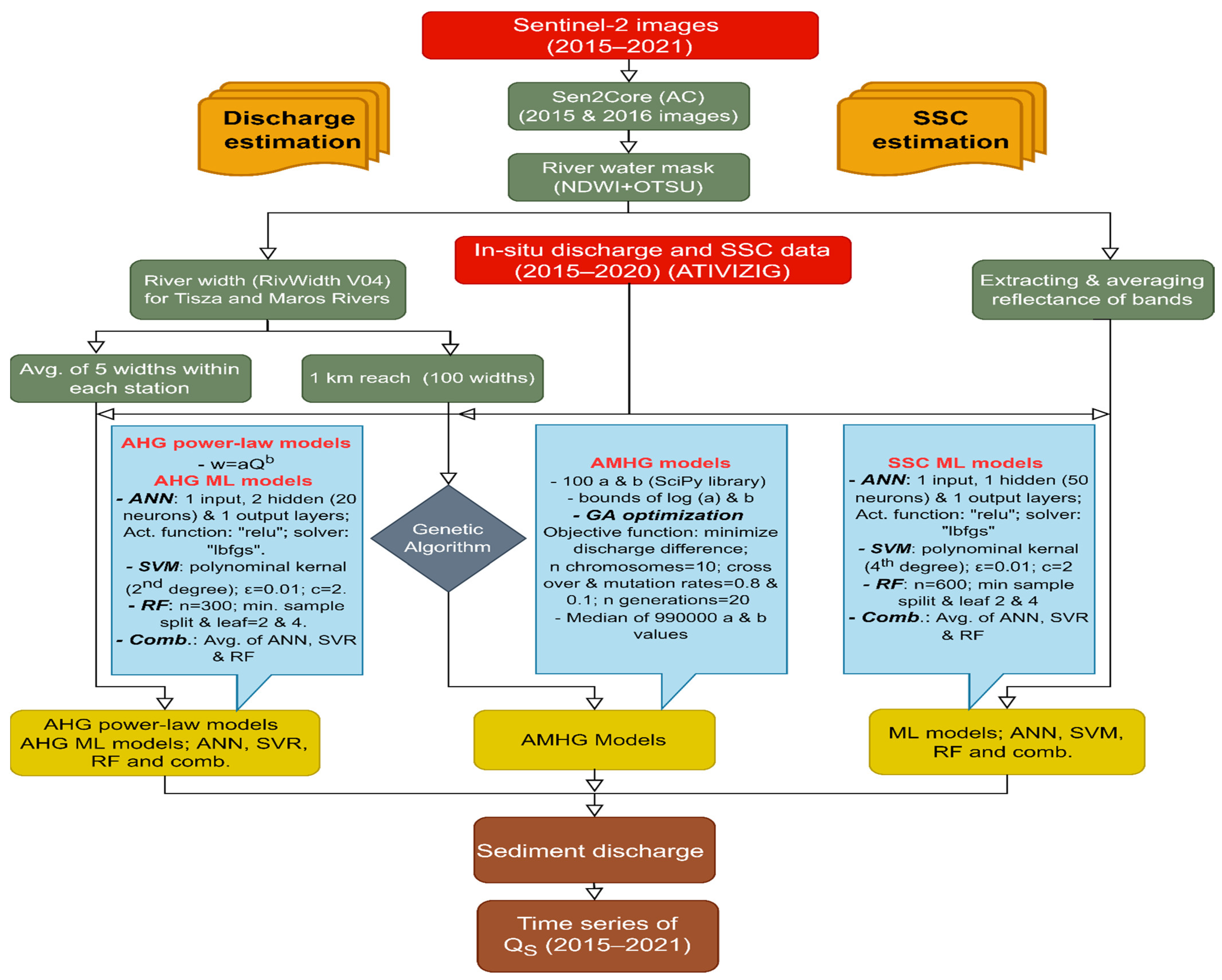
2.4. Pre-Processing of the Satellite Images

All obtained satellite images were available in level 2A (i.e., atmospherically corrected), except those acquired in 2015 and 2016. Thus, the Sen2Core 2.6 plugin, integrated into SNAP 8.0 software [74], converted these images from level 1C to level 2A.

Afterward, all images were resampled into 10 m spatial resolution and clipped within the study area (Figure 1) to reduce the processing time. The water pixels of the rivers were extracted from the images by applying the Normalized Difference Water Index (NDWI; [75]); furthermore, the OTSU thresholding method introduced by Nobuyuki Otsu [76] was applied to obtain the threshold of the NDWI automatically based on the histogram. The scikit-image library in Python was used to apply the OTSU method.

2.5. Water Discharge Estimation

As we aim to estimate sediment discharge from satellite images, various models were built to estimate the water discharge and the suspended sediment concentration based on in situ measurements and Sentinel-2 images. The entire methodology applied in the study to estimate sediment discharge was summarized (Figure 4).

2.5.1. At-a-Station Hydraulic Geometry (AHG), Power–Law, and Machine-Learning Models

At-a-station hydraulic geometry (AHG) is applied at any given cross-section of a natural stream, and it refers to the power–law relationship (Equations (1)–(3)) between water discharge and some hydraulic parameters, such as water depth, width, and velocity (Leopold and Maddock, 1953).

$$w=a{Q}^b; log\left(w\right)= log\left(a\right)+b.log\left(Q\right)$$

(1)

$$d=c{Q}^f; log\left(d\right)= log\left(c\right)+f.log\left(Q\right)$$

(2)

$$v=k{Q}^m; log\left(v\right)= log\left(k\right)+m.log\left(Q\right)$$

(3)

where w is water surface width, d is mean water depth, v is mean water velocity, Q is water discharge, a, c, and k are numerical coefficients, and b, f, and m are exponents of the equations.

The main differences between the derived equations for any cross-section are the values of the coefficients and exponents. It can be noticed that the multiplication of these coefficients $\left(a.c.k\right)$ and the sum of the exponents $\left(b+f+m\right)$ are equal to 1.

This study focuses on the relationship between water width and discharge, as the satellites, with their continuous observation of the ground, can be employed to produce a time series of water width for any river. The selected satellite images for the study area (i.e., Tisza River: 29 images; Maros River: 27 images) were utilized to produce a time series of the river width at the three gauging stations (Figure 1). Five widths spaced at ±10–20 m upstream and downstream of the original cross-section were measured and averaged to reduce the error, which could arise from a single width measurement (Figure 3a–c). The RivWidth V04 software [Pavelsky and Smith [77] (http://uncglobalhydrology.org/rivwidth/; accessed on 2 January 2022)] was used to measure the river width of the Tisza and Maros Rivers (at every 10 m). Afterward, the calculated width and the corresponding discharge at the three stations were fitted by a power–law function in Python using the curve fit function in the SciPy library.

The AHG theory was combined with the machine-learning algorithms; thus, the artificial neural network (ANN), support vector machine (SVM), random forest (RF) algorithms were employed to produce predictive models of water discharge based on the time series of width. The train-test-split function in the Scikit-learn library was used to divide the data into 80% for calibration and 20% for validation.

The artificial neural network (ANN) consists of three layers: input layer, hidden layer, and output layer [78]. Each layer contains several cells (neurons), which receive a signal (impulse) from the preceding neuron to deliver their result after performing some transformations into the subsequent neuron. These neurons are connected by weights, which are randomly selected at the beginning of the training process, and then it updates at every iteration until reaching the optimum weights [79]. The neural network in the scikit-learn library in Python was used to build the discharge model. One input layer containing the width values, two hidden layers with 20 neurons each, and one output layer producing the estimated discharge were applied. The rectified linear unit (relu) activation function, which controls the weighted sum of the inputs to feed it to the subsequent neuron, was applied for the hidden layers. The “relu” function returns the same input value in all cases, except for the values ≤0, as it returns zero [f(x) = max (0, z)], thus it avoids the saturation problem in other activation functions (e.g., sigmoid and tanh). The limited-memory Broyden–Fletcher–Goldfarb–Shanno (lbfgs) solver, which optimizes the weights of every neuron to minimize the cost function, was also applied to the hidden layers. The “lbfgs” updates weights by calculating the inverse of the Hessian matrix. The maximum number of iterations was set to 200.

The support vector machine (SVM) finds the best fit line (hyperplane), which passes through the maximum number of the fitted points [80]. However, the main difference between the SVR and the other regression models is that these models try to find the best fit line, which minimizes the square error between the fitted line and points. Meanwhile, the SVR gives some tolerance to the solution, as it tries to find the best fit line within a threshold value (ε), which increases the chance of obtaining better solutions [81]. The kernel is responsible for finding the hyperplane, especially in problems with higher dimensional space. This study utilized the SVR in the scikit-learn library in Python to produce the discharge model. The polynomial kernel (second degree) was applied; the ε was set to 0.01 and the regularization parameter (c) to 2.

The random forest (RF) was introduced by Breiman [82]. The core of the RF is the decision tree (DT) algorithm, as the RF consists of many DTs working in parallel. The mechanism of the RF is that the input features of data are divided into several DTs. Then, every tree gives its prediction based on the included features, and the final prediction of the RF is the average of all DTs results. The RF avoids overfitting, which could result in a single DT; moreover, it can enhance the accuracy of the model. Many hyperparameters can be tuned to achieve the best performance of the RF model, such as the number of estimators, the maximum feature, minimum sample split, and minimum sample leaf. Our study used the random forest regressor module in the scikit-learn library in Python to build the discharge model. The number of estimators was set to 300, the maximum feature to auto mode, the minimum sample split to 2, and the minimum sample leaf to 4. The criterion used to control the quality of the split was the mean square error (mse).

The machine-learning (ML) models were integrated by averaging their results to produce a combined model. The combination process was implemented in Python. All the settings and parameters implemented in these ML algorithms were applied after fine tuning the hyperparameters until reaching the best available results.

2.5.2. At-Many-Stations Hydraulic Geometry (AMHG) Models

Based on Leopold and Maddock [12], the water width at any river cross-section is correlated with the discharge by a power–law relationship with a specific coefficient a and exponent b (Equation (1)). However, Gleason and Smith [31] discovered that if more than one cross-section is considered, their coefficients a and exponents b are not randomly related to each other; instead, a log-linear relationship could represent their relationship. It was coined as “at-many-stations hydraulic geometry” (AMHG). Suppose coefficient a and exponent b are optimized to minimize the discharge difference between the cross-sections. The reach discharge can be obtained with better accuracy than applying the classical hydraulic geometry AHG, as the estimation is based on several cross-sections [2].

In this study, 1 km long reaches at the three gauging stations were considered, where the stations are located at the middle of the reach (Figure 3). Then, a time series of water width for 100 transects at each gauging station was produced by the RivWidth software (Figure 3a–c). For every transect, a power–law relationship was fitted between the water width and its corresponding discharge at a particular date (which is the same discharge for all cross-sections). The fitting process was performed in Python using the curve fit function in the SciPy library, which produced 100 a and b values for every gauging station. A log-linear relationship was established between the log (a) and b; then, their limits were identified.

The optimization process of a and b values was performed by the genetic algorithm (GA) [83]. The GA depends on biologically inspired operators, including selection, crossover, and mutation, to develop high-quality solutions to optimization problems. The GA has an objective function, which maximizes or minimizes its value by selecting individuals (solutions) from a population. Every solution is called a chromosome, which consists of a number of genes [84]. Initially, random chromosomes are drawn from the population; then, they are passed through selection, cross-over, and mutation for a user-defined number of generations to finally produce the best solution to the problem.

For every station, the GA was applied between every pair of cross-sections (every cross-section is paired with the 100 cross-sections), with an objective function of minimizing the discharge difference between every pair. The population bounds of a and b values were defined based on the log-linear relationship produced previously, and the number of chromosomes was set to 10. Every chromosome contains four genes, which are the a and b values for every cross-section. The GA starts the optimization process by selecting ten chromosomes randomly from the population pool. Then, these chromosomes are combined with the water width to check the validity of the selected chromosome, as it should produce a reasonable discharge value between the minimum and maximum discharge of the river. The chromosome that produces a discharge outside the discharge limit is replaced until reaching ten valid chromosomes. The river discharge bounds can be identified based on the historical discharge values for the river or estimated empirically by Equations (4) and (5) [31]. The minimum and maximum discharge for the Tisza River were set to 50 m³/s and 4000 m³/s, while those for the Maros were 10 m³/s and 850 m³/s, respectively.

$$Q_{min}=w_{min}\times 0.5 \mathrm{m} \left(depth\right)\times 0.1 \mathrm{m}/\mathrm{s}\left(velocity\right)$$

(4)

$$Q_{max}=w_{max}\times 10 \mathrm{m} \left(depth\right)\times 5.0 \mathrm{m}/\mathrm{s}\left(velocity\right)$$

(5)

where $w_{min}$ and $w_{max}$ are the minimum and maximum observed width of the river during the studied period.

The ten chromosomes are then ranked according to their fitness (discharge conservation) in a process called selection. Afterward, each chromosome has a chance to crossover with another chromosome or to mutate. The crossover means that certain genes in the chromosome can exchange their values with genes in another chromosome, while the mutation means that a few genes can be randomly altered to make sure that additional solution is added, which can be helpful in case of bad solutions in the existing chromosomes. The crossover rate is set to 0.8 and the mutation rate to 0.1 [31]. The altered chromosomes are reranked again based on their new fitness, and the least fit five chromosomes are excluded and replaced with another five from the population space. The first generation is passed when the chromosomes pass these previous steps (selection, crossover, and mutation). In our study, we applied 20 generations for every cross-section pair.

The GA was applied to all possible pairs of cross-sections within the 1 km reach, which resulted in 990,000 (Equation (6)) estimates of a and b values for every cross-section.

(n² − n) × 100

(6)

where n is the number of cross-sections (100 in our study).

Then, the median a and b values for every cross-section were calculated and applied as the final optimized constants. The reach discharge was calculated by estimating the discharge for every transect (considering the optimized a and b and the water width); then, the median of the estimated discharges for every transect (100 discharge value) was considered as the reach discharge. The developed GA code in our study in Python is available at this respiratory: AMohsenMetwaly/Genetic-Algorithm (github.com; accessed on 2 January 2022).

2.6. Suspended Sediment Estimation

The ANN, SVM, and RF algorithms and their combination were applied to produce suspended sediment concentration (SSC) models for the Tisza and Maros Rivers. The models for the Tisza were built based on the in situ measurements of suspended sediment at Szeged and the corresponding 29 Sentinel-2 satellite images. Similarly, the Maros models were built based on the suspended sediment measurements at Makó and the corresponding 27 satellite images. The suspended sediment concentrations were available at five verticals (red or green lines; Figure 3). The whole cross-section was divided into five segments, in such a way that the location of the suspended sediment vertical (the midpoint between the high (red vertical) and low (green vertical) stages) lies approximately at the middle of every segment (Figure 3). Then, the average of the reflectance values of the images at these five segments was extracted and correlated with its corresponding suspended sediment concentration using ANN, SVM, and RF algorithms. Bands 2, 3, 4, 5, 6, 7, 8, and 8a of the Sentinel-2 images were considered as independent variables. The reflectance and SSC data were divided; 80% of the data were selected for calibration and 20% for validation by the train-test-split function in the scikit-learn library.

Concerning the selected hyperparameters for every model, in the artificial neural network (ANN) model, one input layer containing the eight selected bands (8 neurons), one hidden layer containing 50 neurons, and one output layer were considered. The “relu” activation function and the “lbfgs” solver were applied for the hidden layer, and the maximum iterations were set to 20. For the support vector machine (SVM) model, the polynomial (fourth degree) kernel was applied; moreover, the ε was set to 0.1 and the regularization parameter (c) to 0.7. In the random forest (RF) model, the number of estimators was set to 600, the maximum feature to auto mode, the minimum sample split to 2, and the minimum sample leaf to 4. The criterion used to control the quality of the split was the mean square error (mse). The average of these ANN, SVM, and RF models was also calculated and considered a combined model.

2.7. Temporal Change of Suspended Sediment Discharge and Performance Evaluation

The suspended sediment discharge can be obtained by multiplying water discharge and SSC [85] (Equation (7)).

$$Q_s=k\times Q\times SSC$$

(7)

where Q_s is the suspended sediment discharge (ton/day), k is a constant referring to units’ conversion (0.0864 SI units), Q is water discharge (m³/s), and SSC is the suspended sediment concentration (mg/L).

The best derived water discharge and SSC models were employed to produce a relatively long time series of the suspended sediment discharge at the three stations (Szeged, Algyő, and Makó). This was performed by applying these models for ungauged dates (122 images) covering the period between July 2015 and May 2021. The daily water discharge data (estimated by rating curves produced by the Lower Tisza Hydrological Directorate (ATIVIZIG) based on daily water stage measurements) at the three stations were used to evaluate the estimated discharge produced by the best discharge model.

The evaluation process between the predicted and measured datasets was performed by three statistical indicators: the coefficient of determination (R²), root mean square error (RMSE), and average distance (AD) from the regression line (Equations (8)–(10)).

$$R^2=1-\frac{{{\displaystyle \sum }}_{i=1}^N{\left(y_i-{\widehat{y}}_i\right)}^2}{{{\displaystyle \sum }}_{i=1}^N{\left(y_i-\overline{y}\right)}^2}$$

(8)

$$RMSE=\sqrt{\frac{{{\displaystyle \sum }}_{i=1}^N{\left(y_i-{\widehat{y}}_i\right)}^2}{N}}$$

(9)

$$AD=\frac{\left|y_i-{\widehat{y}}_i\right|}{N}$$

(10)

where $y_i$ is the observed value, ${\widehat{y}}_i$ is the predicted value by a given model, $\overline{y}$ is the mean of the observed values, and N is the total number of observations.

3. Results

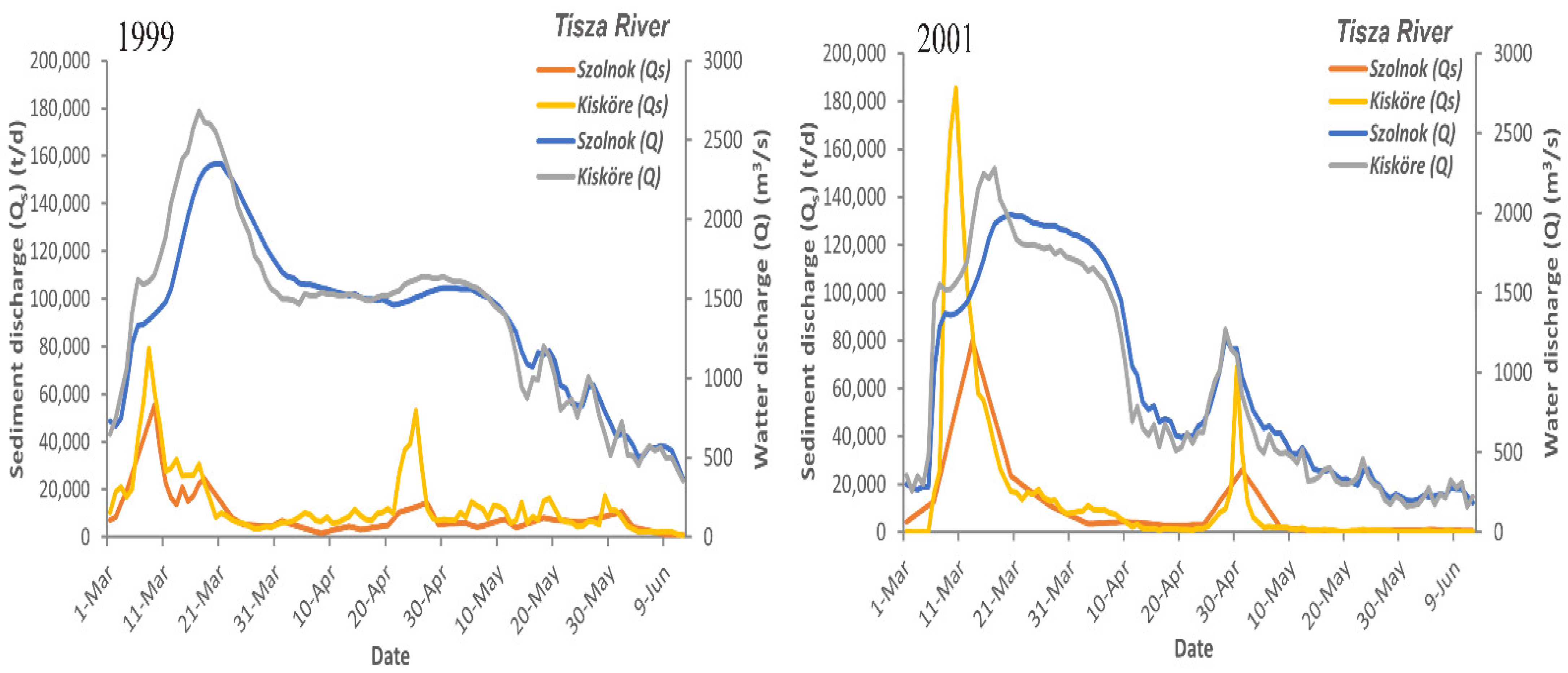
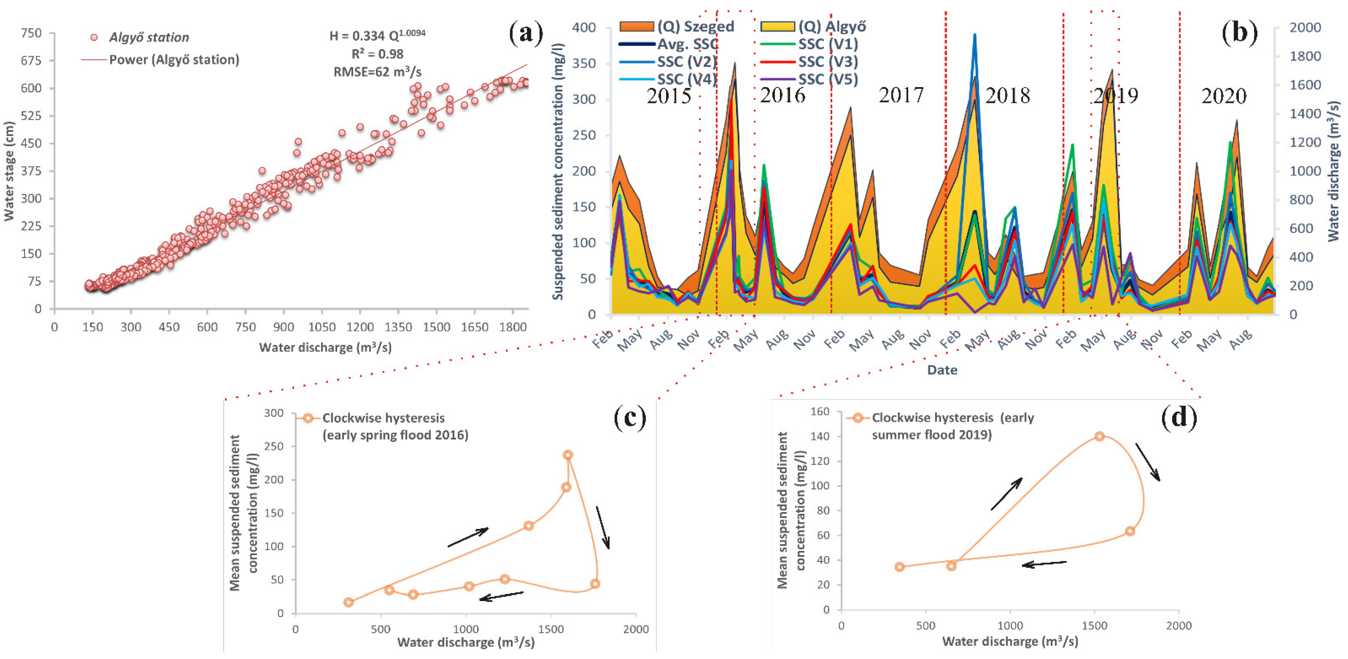
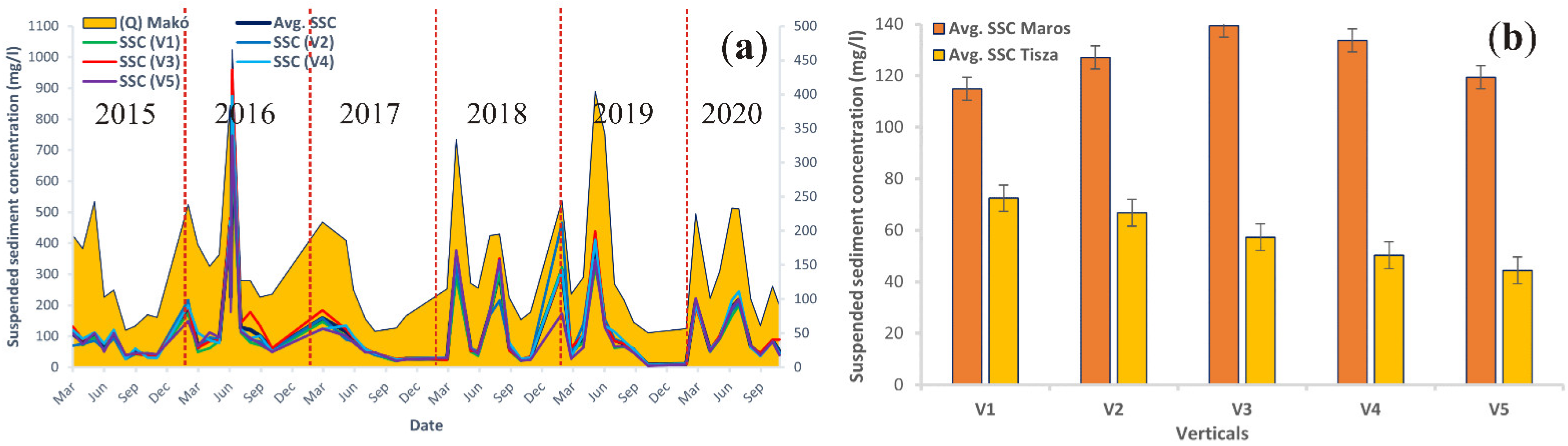
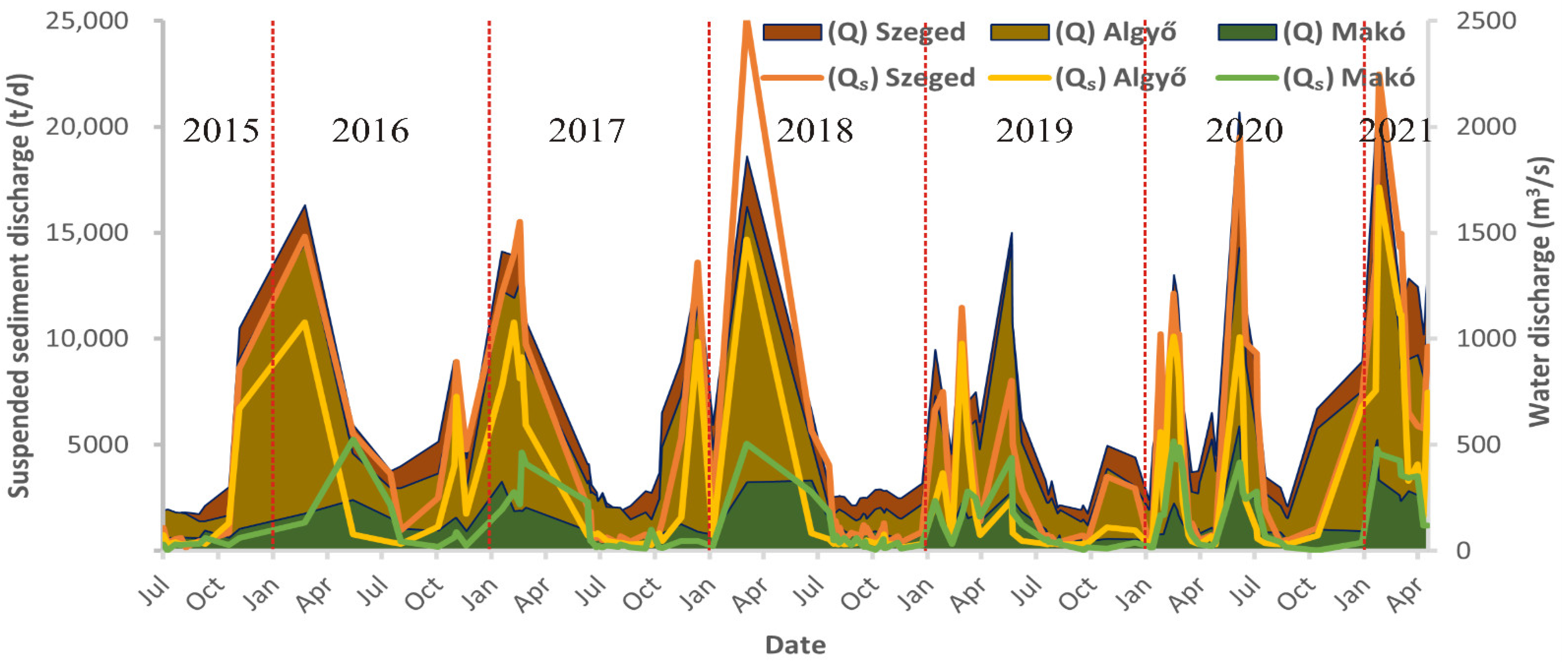
3.1. Temporal Change of Water Discharge and Suspended Sediment Concentration

The rating curve for the Algyő fluviometer (Tisza) was produced based on the daily water stage and discharge data between January 2020 and May 2021, with a coefficient of determination (R²) of 0.98 and RMSE of 62 m³/s (Figure 5a). The derived power–law equation was employed to estimate the discharge at Algyő for the ungauged periods (February 2015–December 2019) based on the measured daily water stages. The temporal change of the water discharge and the SSC (2015–2020) based on the monthly in situ measurements is depicted for the Tisza (Figure 5b) and Maros Rivers (Figure 6a). The average discharge of the Tisza at Algyő (575.2 m³/s) is always lower than at Szeged (702.6 m³/s), as the Szeged gauging station is located downstream of the confluence of the Tisza and the Maros. These discharge values are approximately four times greater than the mean discharge of the Maros River (Makó:157.3 m³/s). However, the average SSC of the Maros River (129.14 mg/L) was approximately two-fold the that of the Tisza River (58.5 mg/L).

The largest flood during the studied period occurred in 2016. The Tisza had its peak discharge in March (Algyő: 1640 m³/s; Szeged:1760 m³/s), but the peak on the Maros (465 m³/s) was recorded in June. Usually, the early spring and summer floods are accompanied by high suspended sediment concentrations; however, their amount can be very different. In addition, the SSC peak in the rivers may lag before or after the discharge peak. On the Tisza, for example, during the early spring flood in 2016, the SSC peak was 248 mg/L (Szeged), but during the early summer flood in 2019, it was only 138.4 mg/L. Another typical phenomenon is that the highest SSC is not necessarily concurrent with the discharge peak. For instance, during the early spring flood of 2016, the SSC reached its peak in February, though the discharge peak was measured in March (Figure 5c,d). A similar temporal pattern (hysteresis) was observed in the early summer flood of 2019. On the other hand, on the Maros River, the highest SSC and the discharge peak are likely to occur simultaneously (Figure 6a), as it occurred in the June 2016 flood. This was also confirmed by the Pearson correlation test, as the correlation coefficient (r) between the average SSC and the discharge was 0.88 for the Maros River, and it was only 0.72 for the Tisza River.

Usually, both rivers have low stages and discharge between August and December. In the Tisza River, the lowest water discharge of the studied period was 141 m³/s (Szeged, August 2015), and it was only 50.6 m³/s in the Maros (Makó, October 2019). In low-stage periods, the SSC usually drops significantly, reaching its lowest values in both rivers, as in October 2019, the Tisza carried only 8.28 mg/L suspended sediment, which was very similar to the data of the Maros (8.19 mg/L).

The in situ SCC measurements were carried out along cross-sections (Figure 3); thus, they provide data on the spatio-temporal changes of the SSC distribution within the channel (Figure 5b and Figure 6a). The data reflect that in the cross-section of the Maros at Makó, the SSC had a more homogeneous distribution than the Tisza River at Szeged. In the case of the Maros, the suspended sediment concentrations at the five verticals were usually more similar than in the Tisza River. However, in the Maros, slight differences could be observed during floods (e.g., June 2016, March 2017, and February 2019) but without any dominant pattern. For instance, sometimes, along the right bank, there were higher SSC than along the left bank (e.g., February 2019) or vice versa (e.g., April 2018). However, the highest SSC concentrations usually occur in the middle, which is related to the highest velocity and stream power. On the other hand, along the cross-section of the Tisza River, a moderate to significant contrast was found in the SSC, especially during floods (e.g., March 2016, March 2017, and April 2018). Unlike the Maros River, the Tisza River showed a dominant SSC pattern: along the left bank, usually a higher SSC was measured than along the right bank. This is related to the confluence location upstream of the Szeged gauging station. This was well presented by the average SSC values of the five verticals (Figure 6b), as they decreased gradually from the left bank (average V1: 72.4 mg/L) to the right bank (average V5: 44.4 mg/L). Meanwhile the highest concentration in the Maros River (Makó station) was observed in the middle (V3: 139.4 mg/L), and both the right and left banks had had similar concentrations (right bank (V1: 115 mg/L and V2: 127.1 mg/L); left bank (V4: 133.8 mg/L and V5: 119.4 mg/L) (Figure 6b)).

3.2. Estimating Water Discharge

To predict water discharge based on the width measured by Sentinel-2 images, the AHG power–law, AHG machine-learning (ML), and AMHG water discharge models were developed; additionally, their results were compared to define the most suitable method for estimating sediment discharge.

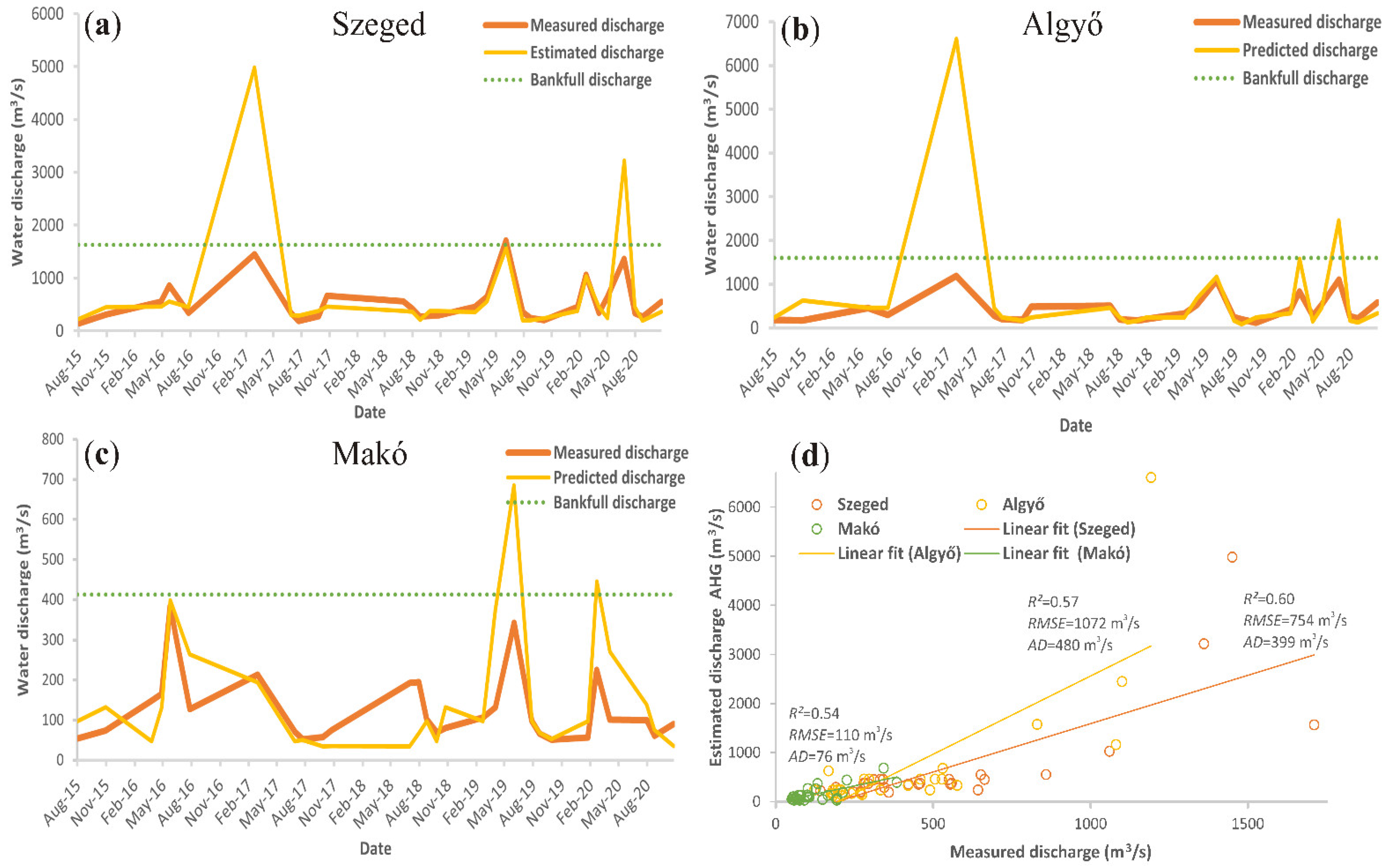
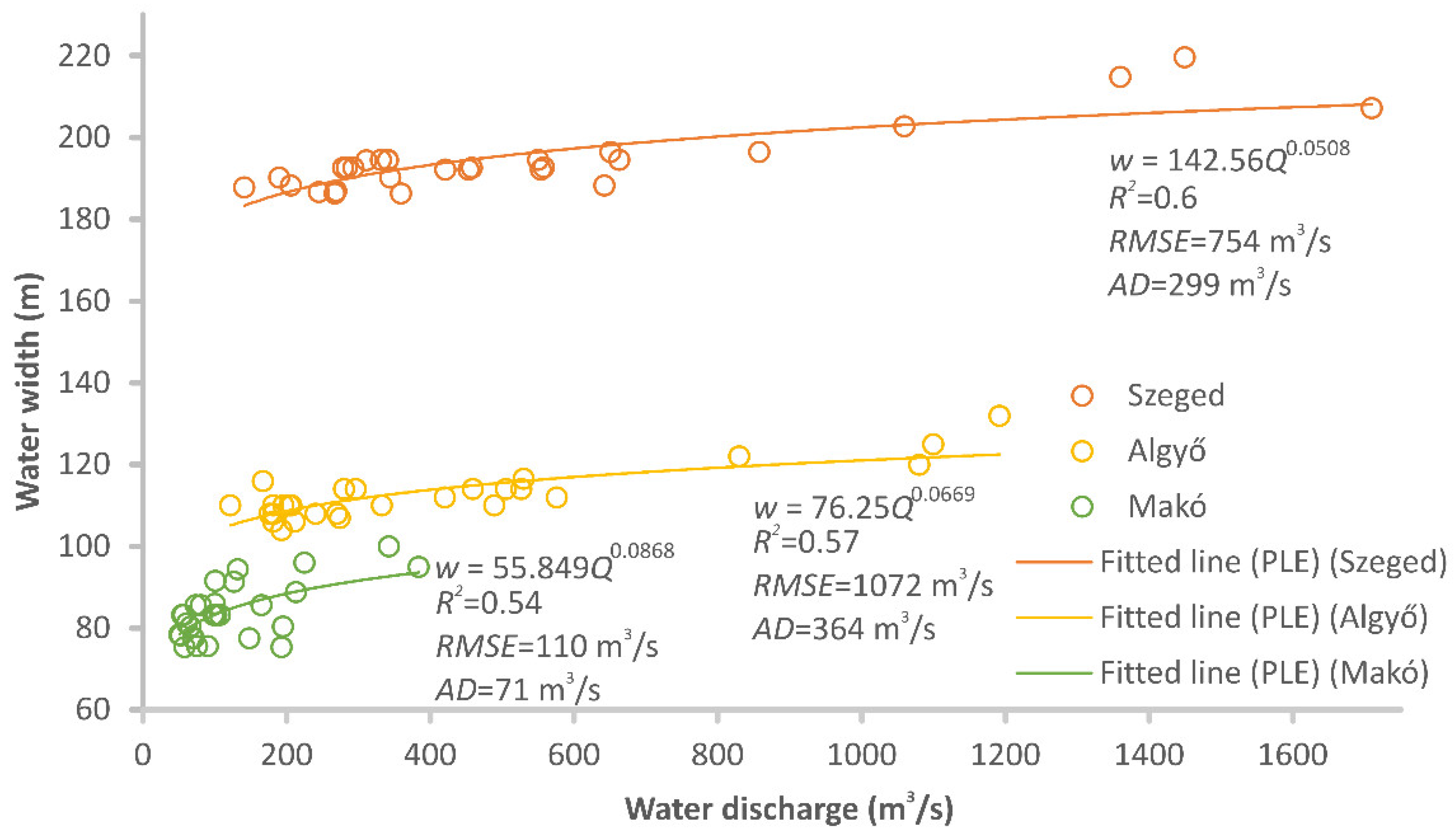
3.2.1. AHG Power–Law Models

The average width of the five transects (Figure 3) at a particular date and the corresponding measured water discharge were fitted by power–law equations for Szeged, Algyő, and Makó gauging stations (see Appendix A, Figure A1). The estimated discharges by the AHG power–law models were compared to the measured discharges, and the R², RMSE, and AD values were calculated (Figure 7). The performance of the AHG power–law model at the three stations was similar; however, it had a slightly better performance at the Szeged station (R² = 0.6) than at Algyő (R² = 0.57) or Makó (R² = 0.54) stations. Usually, the models gave good predictions for the discharges below the bankfull (Szeged: 1628 m³/s, Algyő: 1600 m³/s, and Makó: 412 m³/s). However, worse predictions were obtained for discharges close or exceeding the bankfull discharge (e.g., floods in March 2017 at Szeged and Algyő, and in June 2019 at Makó), where the models significantly overestimated the discharges. Although the AHG power–law models of Szeged and Algyő stations had the highest R², they produced high RMSE (Szeged: 754 m³/s; RMSE/mean observed: 1.07; Algyő: 1072 m³/s; RMSE/mean observed: 1.8) due to their significant overestimation of high discharges (e.g., March 2017 and July 2020).

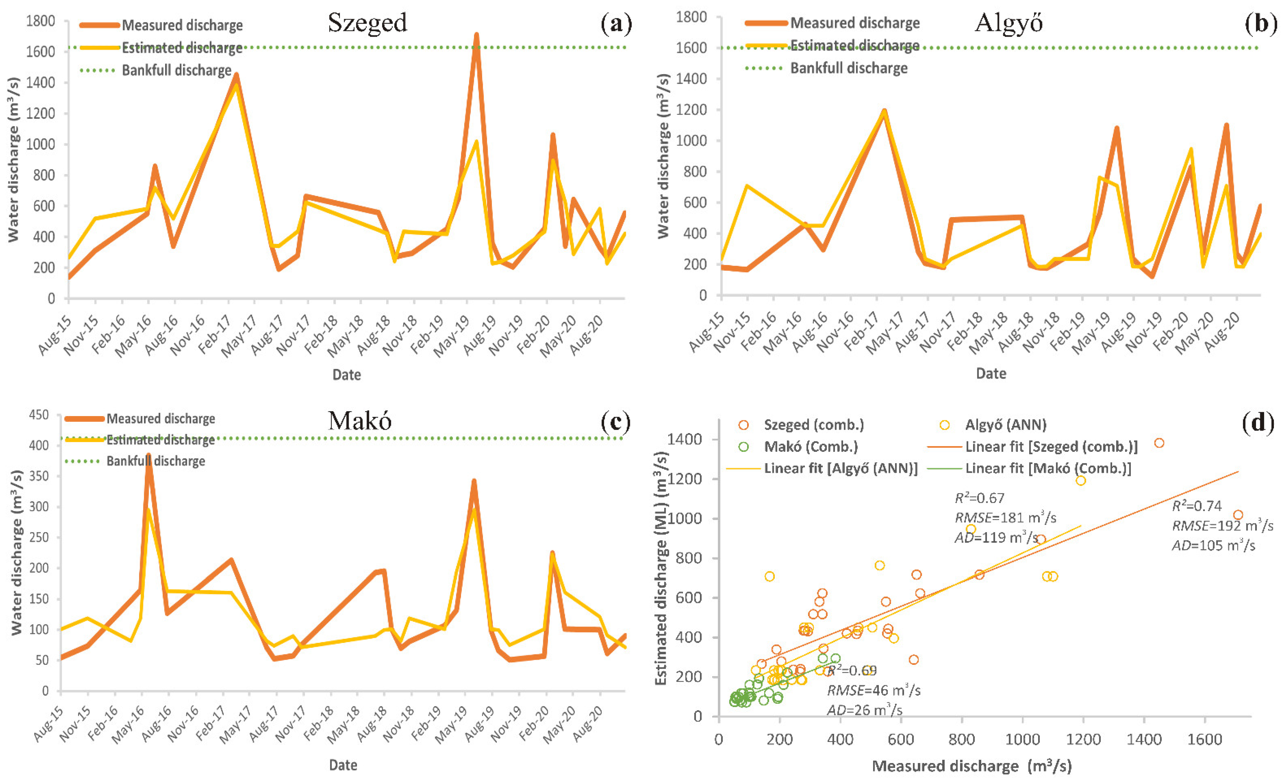
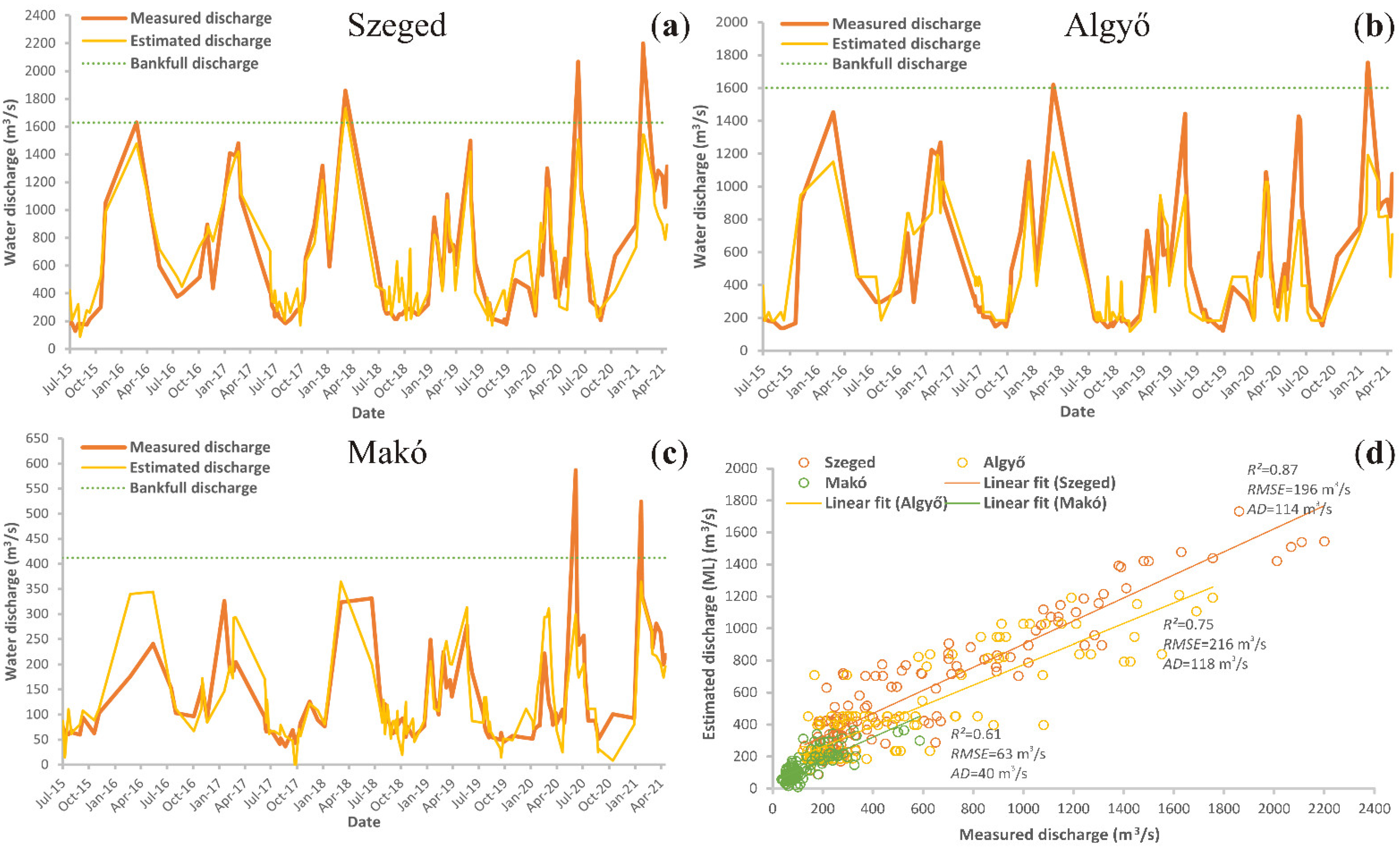
3.2.2. AHG Machine-Learning Models

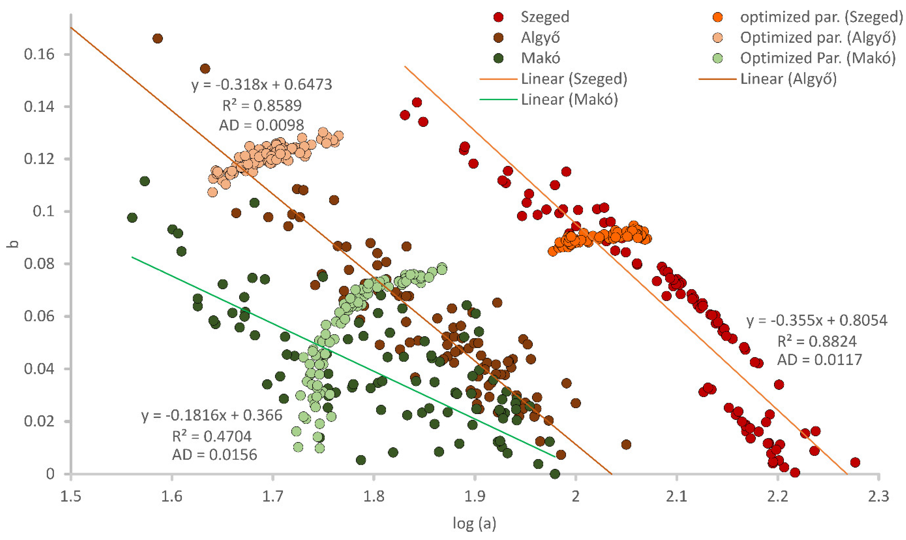
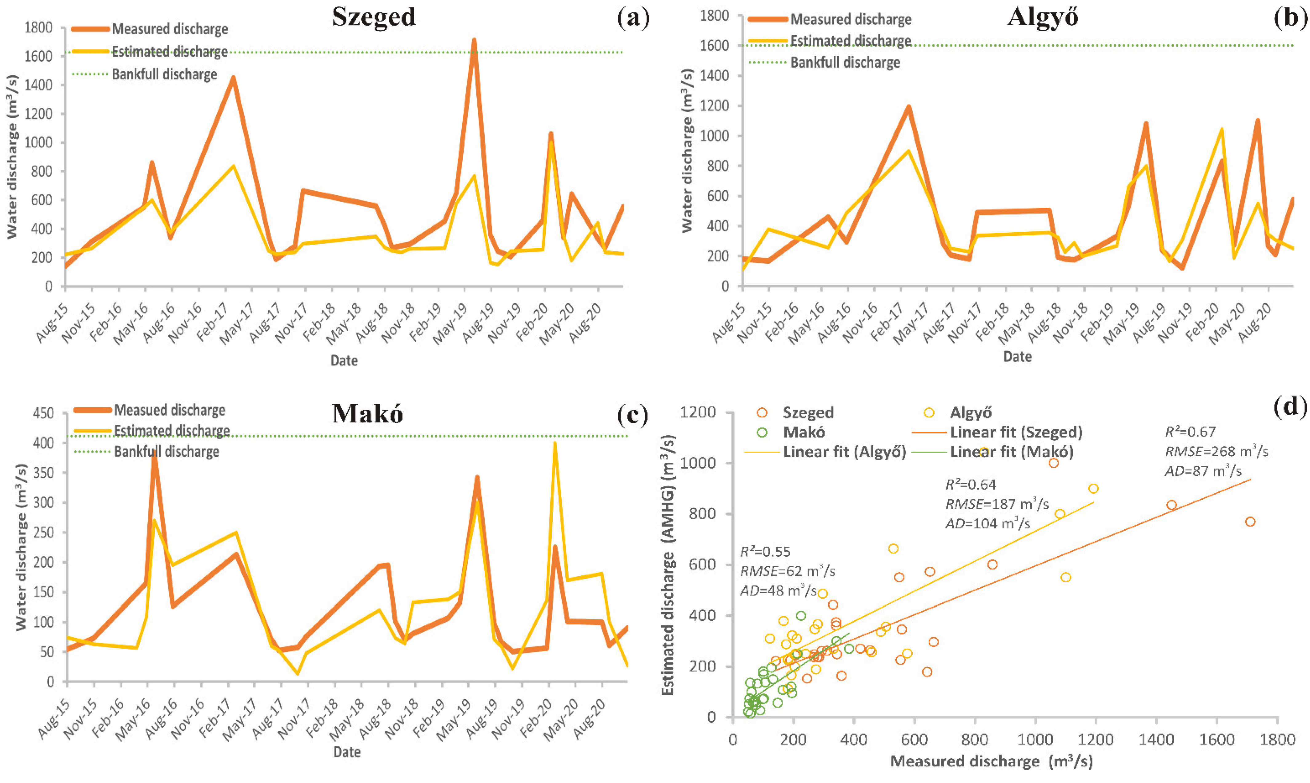
The SVR, RF, and ANN algorithms were calibrated by 80% of the data and validated by 20%. A combined model considering the average of their predictions was also derived. The R² and RMSE for every model at the three stations were produced based on the validation dataset (

Table 1. The results of the evaluation metrics (R² and RMSE) for estimating water discharge using support vector regression (SVR), random forest (RF), artificial neural network (ANN) algorithms and their combined model based on the validation dataset (20%) for Szeged, Algyő, and Makó stations. The models in bold refer to the best AHG machine-learning model at every station based on the R² values. The R² and RMSE of the AHG power–law and AMHG methods were added for the purpose of comparison.

Station	AHG Machine-Learning			AHG Power–Law		AMHG
	Algorithm	R2	RMSE (m3/s)	R2	RMSE (m3/s)	R2	RMSE (m3/s)
Szeged	Support Vector Regression (SVR)	0.65	131.97	0.6	754	0.67	268
	Random Forest (RF)	0.71	154.12
	Artificial Neural Network (ANN)	0.76	119.94
	Combined model	0.83	99.9
Algyő	Support Vector Regression (SVR)	0.72	98.92	0.57	1072	0.64	187
	Random Forest (RF)	0.68	123.55
	Artificial Neural Network (ANN)	0.79	123.28
	Combined model	0.77	107.84
Makó	Support Vector Regression (SVR)	0.85	33.65	0.54	110	0.55	62
	Random Forest (RF)	0.81	25.37
	Artificial Neural Network (ANN)	0.85	30.98
	Combined model	0.88	25.93

). The performance of the machine-learning models (SVR, RF, and ANN) was promising, as the R² ranged between 0.65 (SVR model—Szeged station) and 0.88 (combined model—Makó station); moreover, the RMSE for Tisza models ranged between 154.12 m³/s (RF model—Szeged station) and 98.92 m³/s (SVR model—Algyő station), and for Maros models between 33.65 m³/s (SVR model—Makó station) and 25.37 m³/s (RF model—Makó station). The models with the highest R² were considered the best performing models for every gauging station; thus, the combined model was considered the best model for Szeged (R² = 0.83) and Makó (R² = 0.88) stations, and the ANN for Algyő (R² = 0.79) station.

The best performing models were applied to predict the discharge for the entire dataset (including the calibration and validation data) at every gauging station (Szeged and Algyő: 29 images; Makó: 27 images). This enabled the comparison of the various adopted methods (i.e., AHG power–law, AHG machine-learning (ML), and AMHG methods) to retrieve water discharge. The predicted and actually measured discharges, in addition to the R², RMSE, and AD data, are depicted in Figure 8. The estimated discharges by the AHG ML models were more consistent with the measured discharges than the AHG power–law models. This was especially the case with high discharges, which were usually overestimated by the AHG power–law models; meanwhile, the AHG ML models gave closer estimations to the measured discharges. This was also reflected in the RMSE results, as in the case of Algyő station it dropped by 80% (from 1072 m³/s to 181 m³/s), at Szeged by 75% (from 754 m³/s to 192 m³/s), and by 58% (from 110 m³/s to 46 m³/s) in case of Makó station compared to the AHG power–law models. Based on the evaluation metrices (Figure 8d), it can be noted that the AHG ML models performed best at Szeged station, followed by Makó and Algyő stations.

3.2.3. AMHG Models

The “at-many-stations hydraulic geometry” (AMHG) method was also tested based on the 100 transects at every gauging station to estimate water discharge. The relationship between the logarithm of the coefficient log (a) and the exponent b based on the 100 transects at every gauging station, and their optimized values by the genetic algorithm (GA), are depicted (Figure 9). All the gauging stations showed a log-linear relationship between log (a) and b. However, the best relationship was achieved at Szeged (R² = 0.88), followed by Algyő (R² = 0.86) stations, and the worst was for the Makó station (R² = 0.47). The optimized coefficients and exponents of the 100 transects at every station seem to be clustered around approximately the middle of the log-linear regression line.

For the Szeged station, the ranges of log (a): 1.83–2.27 and b: 0–0.141 were used as an input for the genetic algorithm, which resulted in optimized coefficients and exponent ranges of log (a): 1.98–2.07 and b: 0.085 and 0.095, which were very convergent and close to the regression line. Similarly, the ranges of log (a): 1.47–2.05 and b: 0–0.209 were used as an input for the GA in Algyő station, and the optimized coefficients and exponents ranges were log (a): 1.64–1.77 and b: 0.107–0.13. On the other hand, the optimized ranges of the coefficients and exponents at Makó (log (a): 1.56–1.98 and b:0–0.111) were wider than the produced ranges in Szeged and Algyő stations (log (a): 1.72–1.87 and b: 0–0.079) due to the decreased log-linear correlations at Makó station.

The estimated discharges by the AMHG method were compared to the measured discharges, and the R² and RMSE for every station were represented (Figure 10). The performance of the AMHG models outweighed the AHG power–law models, as the R² was improved by ≈5%, on average, and the RMSE was declined by ≈65%, on average. Meanwhile, their performance was closer or slightly lower than the AHG ML models, as the R² was 8% (on average) lower than that in the AHG ML models (average R² = 0.7), and the RMSE was 19% higher (AHG ML: average RMSE: 139.67 m³/s). Although the AMHG models overcame the significant overestimation of the AHG power–law models for high discharges, they usually underestimated the real discharges (e.g., March 2017 and June 2019 at Szeged and Algyő stations; June 2016 and June 2019 at Makó station) but with lower rates. The AMHG gave good predictions for low and medium discharges. The AMHG model at the Szeged station was the best (R² = 0.67), followed by Algyő (R² = 0.67) and Makó (R² = 0.55) stations. The same order was observed in the case of the AHG power–law models.

Based on the performance in terms of R², RMSE, and AD of the AHG power–law, AHG ML, and AMHG models at the three gauging stations, it can be noticed that the AHG ML and AMHG were the most reliable methods to retrieve the discharge, while the AHG power–law was the least accurate method. Usually, the water discharge estimations at Szeged were better than at Algyő, and they had the lowest quality at Makó. This could be inferred from the gradient of R² and AD, as they showed the best values at Szeged and the worst at Makó (Figure 7, Figure 8, Figure 9 and Figure 10). It reveals the significant role of the river channel size and cross-sectional shape in the applied water discharge estimation methods.

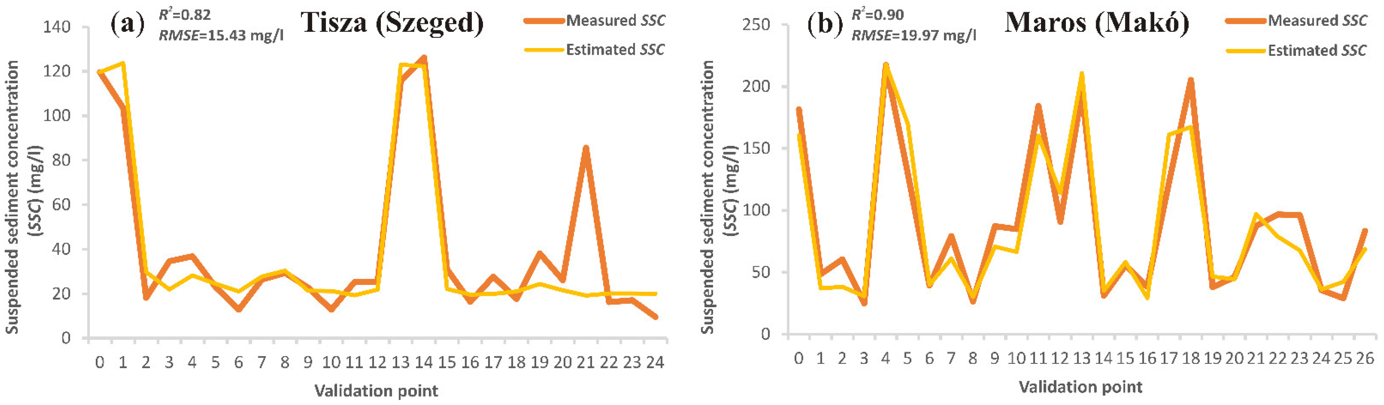
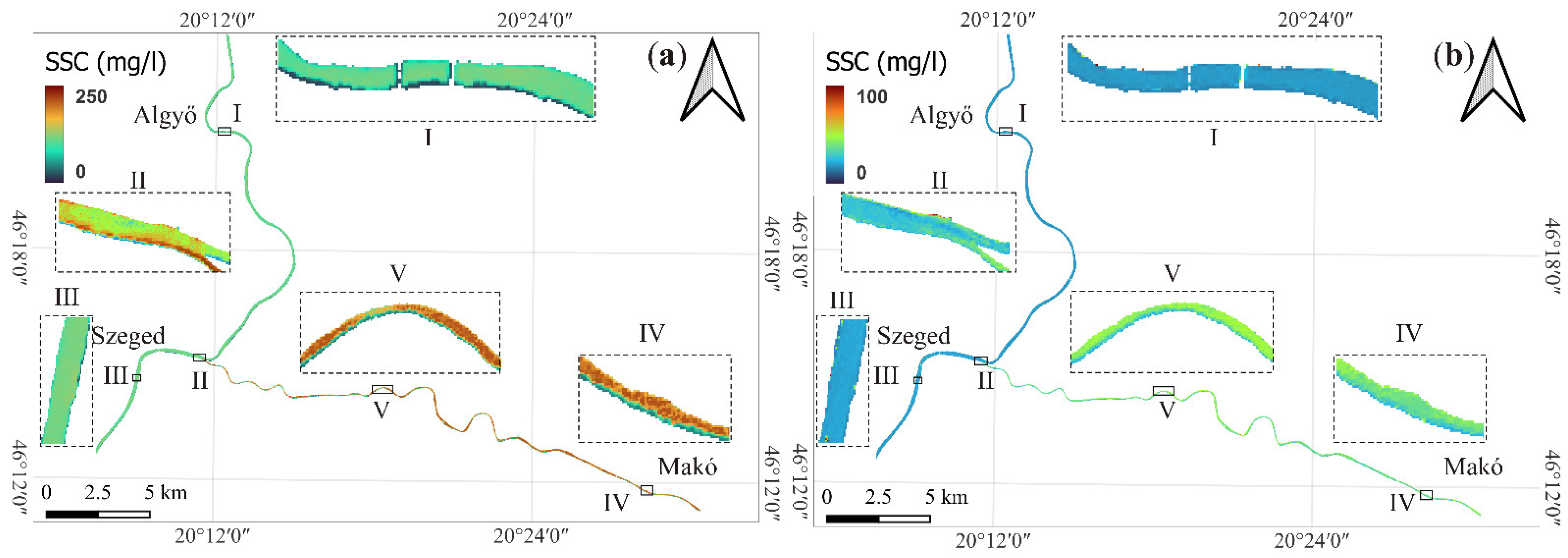
3.3. Estimating Suspended Sediment Concentration

The spectral signatures of water in the Tisza (Szeged station) and Maros (Makó station) Rivers were analyzed to estimate their suspended sediment concentrations. The spectral signature based on the average of reflectance during low and high stages is depicted (Figure 11a). Furthermore, it was also represented for low and high stages separately for both rivers, as it is expected that they would produce different signatures due to the significant variations in SSC during these hydrological situations (Figure 11b). Generally, the reflectance of the Maros River was higher than the Tisza River; furthermore, the reflectance at high stages in both rivers was higher than at low stages (Figure 11a,b). Both rivers showed low reflectance at the blue band (B2), which refers to the turbidity of water, as clear water has high reflectance at this band [2]. Furthermore, a decreasing trend in the reflectance can be noticed between the red edge 2 (B6) and SWIR 2 (B12) bands. The highest reflectance occurred between the green (B3) and red edge 1 (B5) bands. The Tisza River showed the highest reflectance at the green (B3) band, while that in the Maros River was at the red edge 1 (B5) band (Figure 11a). Similarly, the green (B3) band had had the highest reflectance at the low stages, and the red edge 1 (B5) at the high stages of both rivers, which indicates the usefulness of the green (B3) band for detecting low SSC and red edge 1 (B5) for high SSC.

The R², RMSE, and RMSE/mean observed of the SVR, RF, ANN, and combined SSC models for the Tisza and Maros Rivers were tabulated (

Table 2. The R², RMSE, and RMSE/mean observed for the applied machine-learning models at the Tisza and Maros Rivers for estimating suspended sediment concentration (SSC) by support vector regression (SVR), random forest (RF), artificial neural network (ANN) algorithms based on the validation dataset (20%). The bold fonts refer to the best performing model for a given river based on the R² value of the applied model.

Station	Algorithm	R2	RMSE (mg/L)	RMSE/Mean Observed
Tisza River (Szeged)	Support Vector Regression (SVR)	0.78	17.28	0.42
	Random Forest (RF)	0.76	15.23	0.37
	Artificial Neural Network (ANN)	0.82	17.96	0.44
	Combined model	0.82	15.43	0.38
Maros River (Makó)	Support Vector Regression (SVR)	0.78	24.9	0.28
	Random Forest (RF)	0.90	19.97	0.22
	Artificial Neural Network (ANN)	0.85	22.72	0.25
	Combined model	0.88	19.75	0.22

). Generally, all the derived models showed good results, as the R² ranged between 0.76 and 0.9, and the RMSE was between 24.9 mg/L and 15.23 mg/L. However, the SSC models of the Tisza River showed slightly lower accuracies than the Maros models, as the average R² of the Tisza models (0.8) was lower than the Maros models (0.85) by 5% (based on the average of all derived models). However, as the Maros River had greater SSC, the average RMSE of the Maros (21.8 mg/L) was slightly higher than the Tisza (16.47 mg/L). The best derived SSC model for the Tisza River was the combined model, followed by the ANN, SVR, and RF models. Meanwhile, the RF was the best in the Maros River, followed by the combined model, ANN, and SVR models. Hence, the combined SSC model in the Tisza and the RF model in the Maros were used to predict the sediment discharge (Q_s).

The measured and predicted SSC by the best models were compared for both rivers based on the validation dataset (Figure 12). The predicted SSC was quite consistent with the measured one for both rivers, especially for the Maros River, as the R² in the Maros was higher than the Tisza by 8% (based on the best derived models for both rivers). Despite the accurate estimations of the derived models, both models tended to slightly underestimate the actual measured SSC, as the mean estimated SSC based on the validation dataset in the Tisza was 38.5 mg/L, contrary to 40.7 mg/L mean measured SSC (percent bias: −5.31%). Similarly, the mean estimated SSC in the Maros was 86.6 mg/L, contrary to the 89.5 mg/L mean measured SSC (percent bias: −3.18%).

Based on the best performing models, the SSC for ca. 20 km long sections of the Tisza and Maros Rivers were calculated. As an example, the spatial distributions of the SSC during high (5 March 2020) and low stages (6 September 2020) were presented (Figure 13a,b). During the high-stage situation (Figure 13a), the average SSC of the Tisza (106.22 mg/L) was 6.3 times greater than at the low stage (16.96 mg/L) (Figure 13b). Similarly, the average SSC of the Maros at the high stage (211 mg/L) was 5.2 times greater than at the low stage (40.8 mg/L). In both hydrological situations, the Maros River had higher SSC than the Tisza River; however, the concentration difference decreased during the high stages, as on the given days, the Maros (211 mg/L) had 2 times higher concentrations than the Tisza (106.22 mg/L), and their difference increased to 2.4 times at low stage (Maros: 40.8 mg/L; Tisza: 16.96 mg/L).

The spatial distribution of the SSC was more homogeneous along the Tisza River’s cross-sections during low stages than the high stages. For instance, during high stages, the highest SSC could be noticed at the middle of the Algyő gauging station (Figure 13(aI)), and it decreased gradually toward the riverbanks; in the meantime, it had almost the same concentrations along the entire cross-section during low stages (Figure 13(bI)). Concerning the Maros River, the SSC was almost the same along the cross-sections during high or low stages (Figure 13(aIV,aV)), Figure 13(bIV,bV); however, the SSC of some pixels along the riverbanks were underestimated due to the tree shadow, which had a drastic impact on this river due to its limited width (average width 126 m). The SSC spatial distribution at the confluence area showed a more complicated spatial distribution than the rivers themselves, as, during high stages, the Maros is usually impounded by the Tisza due to higher momentum of the Tisza. Thus, it extended longitudinally with limited width (Figure 13(aII,aIII); meanwhile, during low stages, the Maros water extended laterally wider than at the high stages (Figure 13(bII,bIII)). However, it mixed faster, as it showed a very limited longitudinal extent compared to the high stages.

3.4. Estimated Suspended Sediment Discharge of the Tisza and Maros Rivers Based on the Derived Models

After evaluating the performance of the three applied methods (i.e., AHG power–law, AHG ML, and AMHG) to estimate the water discharge from the Sentinel-2 satellite images, the best performing AHG ML models were applied to predict the water discharge at Szeged, Algyő, and Makó gauging stations between July 2015 and May 2021. Similarly, the combined SSC model was utilized to predict the SSC in the Tisza River (Algyő and Szeged stations), whereas the RF was applied to estimate the SSC of the Maros River (Makó station).

A time series of the suspended sediment discharge (Q_s) at Algyő, Szeged, and Makó stations between July 2015 and May 2021 based on 122 Sentinel-2 images was created (Figure 14). Although the SSC in the Maros River was usually 2–3 times greater than in the Tisza River, the suspended sediment discharge of the Tisza River was 2–3.5 times greater than that of the Maros River. This is because of the elevated discharge of the Tisza River (four-fold) compared to the Maros River. Usually, the suspended sediment discharge of the Tisza upstream of the confluence (at Algyő average Q_s= 2584 t/d) was greater than that of the Maros (at Makó average Q_s = 1264 t/d). However, downstream of their confluence, the suspended sediment discharge at Szeged increased considerably (Q_s= 4385 t/d). On the other hand, in some hydrological situations, the Q_s at Makó was greater than the Q_s at Algyő (e.g., June and August 2016, July 2017, July–August 2018, June–July 2019). This usually occurs during low stages, when the SSC in the Maros River increases due to small flood waves compared to the very low SSC in the Tisza River.

Usually, the temporal changes in suspended sediment discharge followed a similar pattern as water discharge; thus, the sediment discharge peaks were observed during floods and the lowest values during low stages. Usually, the Q_s peak at the Maros River was concurrent with that in the Tisza River; however, in some cases, it preceded (e.g., February 2019 and February 2021) or followed (e.g., June 2016 and March 2017) the peak Q_s of the Tisza. As the Szeged station is located on the Tisza River downstream of the confluence of the Tisza and the Maros, here, sediment discharge differed significantly compared to the upstream sections. As a result, sometimes, the Q_s peak at Szeged station shifted forward (e.g., March 2017) or backward (e.g., February 2021), the Q_s at Algyő following the Q_s of the Maros River.

4. Discussion

Although sediment discharge monitoring in rivers is an important issue from several aspects (hydrology, geomorphology, ecology, contamination control), many rivers are still ungauged, and the number of gauged rivers is being decreased because these measurements are labor intensive and expensive [19]. In the meantime, remote sensing with its large-scale coverage and frequent revisiting could be employed to monitor rivers effectively. Therefore, this study aimed to estimate suspended sediment discharge by Sentinel-2 images, considering the medium-sized Tisza River and its tributary Maros River in central Europe as a case study. Therefore, various methods were applied to estimate the water discharge and the suspended sediment concentration (SSC); thus, the suspended sediment discharge could be calculated.

4.1. Suspended Sediment and Water Discharge Conditions in the Rivers Based on In Situ Measurements

The measured SSC in the Maros was twice as much as that in the Tisza River upstream of their confluence because the catchment of the Maros consists of highly erodible rocks, and there are intensive mining activities in Transylvania [86]. The temporal change of the SSC was in good agreement with the water discharge (Tisza River: r = 0.88; Maros River: r = 0.72), as the highest SSC were detected during floods and the lowest during low stages (Figure 5b and Figure 6a). However, a hysteretic behavior in the relationship between the SSC and Q was observed in both rivers, especially in the Tisza River; the SSC peak usually precedes the water discharge peak (clockwise hysteresis). This was also observed at the Middle Tisza (Szolnok and Kisköre) based on five years (1998–2002) of measurements of the SSC and water discharge conducted by Csépes et al. [69]. A similar phenomenon was reported in many rivers, such as the Save River, France [87], Rybárik Basin, Slovakia [88], Chabagou Creek, China [89], and Holbeck Basin, England [90]. This clockwise (positive) hysteresis could develop due to the availability of sediments in the channel and in the neighboring areas at the beginning of the flood wave [87], which can be reflected in a higher SSC in the rising limb of the storm hydrograph than the falling limb.

The lateral distribution of the measured SSC at the cross-section of the rivers usually corresponds to the velocity distribution [91]. This was the case for the Makó and Algyő gauging stations, thus upstream of the confluence. However, downstream of the confluence of the Tisza and Maros Rivers (at Szeged), the SSC was the highest at the low velocity left bank, and it decreased toward the right (concave) bank. This unusual situation occurred due to the special spatial configuration of the gauging station just 4.1 km far from the confluence. As the Maros joins from the left side, usually with higher SSC, at the gauging station, the waters of both rivers are still mixing, as the complete mixing requires a much longer distance (e.g., 15–150 km, according to Jirka [92]). This result is consistent with Mohsen et al. [47], who investigated the spatio-temporal dynamism of the mixing process in the confluence of the Tisza and Maros Rivers, reporting that the water of the Maros could be extended to the Szeged gauging station in certain hydrological situations (i.e., Q_Makó/Q_Szeged = 0.28–0.51; and their slope difference is ΔS_Tisza-Maros = −17.7–8.2).

4.2. Performance of the Water Discharge Models

According to our study, the combination of the hydraulic geometry theory and remote sensing was very useful, as following the best described method, the water discharge could be estimated with an accuracy of Tisza: 186.5 m³/s (RMSE/mean observed = 0.29) and Maros: 46 m³/s (RMSE/mean observed = 0.29). Thus, it could be a useful tool to estimate the water discharge along ungauged sections. However, selecting the appropriate reach is critical for obtaining representative discharges. This was also reported by Flores et al. [2], as they applied the Bayesian AMHG method to obtain water discharge at various reaches (i.e., braided, relatively straight, and low sinuosity); the accuracy varied, but the best accuracy was reached at relatively straight and low sinuosity reaches. Although the three tested reaches in our study were relatively straight (Figure 3), the accuracy varied too, as Szeged (RMSE = 192 m³/s; RMSE/mean observed =0.27; R² = 0.67; AD = 197 m³/s) and Algyő (RMSE = 181 m³/s; RMSE/mean observed = 0.31; R² = 0.62; AD = 234 m³/s) gauging stations in the Tisza River gave the highest accuracy, while the lowest was recorded at Makó (RMSE = 46 m³/s; RMSE/mean observed = 0.29; R² = 0.59; AD = 50 m³/s) gauging station in the Maros River. This could be related to the channel size and the hydraulic geometry of the selected reach, as the estimated width by remote sensing of the narrow Maros (average width at Makó: 93.8 m) had a greater error than of the wider Tisza (average width at Szeged: 203.1 m; and at Algyő: 113 m). In addition, the Tisza has V-shape-like cross-sections, whereas the Maros has a trapezoidal or a near rectangular shape (Figure 3). From the point of view of the width–discharge relationship, the V shape channels provide better hydraulic geometry than rectangular channels [12]; therefore, the water discharge estimation could be more precise. On the other hand, the bankfull level is considered one of the main limits of the hydraulic geometry theory (discharge–width relationship), as the geometrical characteristics of the cross-section of the channel change above this level due to covering the floodplains. Therefore, the derived models usually underestimate (e.g., AHG ML and AMHG method) or overestimate (e.g., AHG power–law method) its actual value, regardless of the selected cross-section, due to losing the hydraulic geometry of the original cross-section.

The performance of the AMHG method outweighed the AHG power–law method, as the average R² for the AMHG models was 0.62 in contrast to 0.57 of the AHG power–law models (based on the three tested reaches). Similarly, the RMSE dropped from 172 m³/s in cased of AMHG models to 645 m³/s in case of AHG power–law models (73% difference). Similar results were reported by Durga Rao et al. [35], who applied the AHG power–law and AMHG methods to estimate water discharge for four main rivers in India using Landsat and Indian remote sensing satellites (IRS) images. According to their data, the Nash coefficients for the AHG power–law and AMHG models were 0.696 and 0.803, respectively. This difference could be explained by the usage of the hydraulic geometry of many cross-sections along the reach in the case of the AMHG method, while only one cross-section was considered in the AHG power–law method. In addition, the AHG method is considered an inherent part of the AMHG method. We developed a novel method by combining the AHG method with machine-learning algorithms, and it gave promising results on water discharge estimation. The results of the AHG ML models were comparable or even better than the AMHG models, as the average R² for the three gauging stations based on the AHG ML method was 0.7 in comparison to 0.62 in the case of the AMHG method; moreover, the RMSE dropped from 172 m³/s (AMHG) to 140 m³/s (AHG ML). The AHG ML models were very stable, as they showed good estimations when they were applied to estimate water discharge for the time series of 122 images (2015–2021), which were totally new data or unseen during the training process (see Appendix A, Figure A2).

The superiority of the AHG ML method can be interpreted by the nature of machine learning itself, as it was mainly developed to give the best possible predictions by employing general-purpose learning algorithms to uncover patterns in data that are frequently large and unmanageable [93]. Unlike the conventional statical regression methods, such as the AHG power–law method, the ML algorithms usually give ambiguous structures, as they learn from the provided dataset [93]. Based on this finding, the AHG ML method can substitute the hydraulic geometry of the multiple cross-sections in the AMHG method; thus, it can avoid the complex optimization process of the coefficients and components in the AMHG, and consequently, larger cross-sections along the river can be monitored.

It is important to note that the accuracy of the derived water width from the satellite images affects the estimated water discharge by the hydraulic geometry method significantly. This mainly depends on the spatial resolution of the images and the extraction method of water pixels. The automatic thresholding of the NDWI using the OTSU method proved its ability as a good tool to extract the river water pixels effectively, as the RMSE for the estimated water width by the satellite images at Szeged gauging station was 8.17 m and 9.9 at Makó gauging station, which was very close to the actual pixel size of the Sentinel-2 images. Thus, applying this method to finer spatial resolution images would produce good estimates for the water width of a river.

4.3. Performance of the Suspended Sediment Models

Based on the spectral signatures of water of the studied rivers, the green (B3), red (B4), and red edge 1 (B5) bands seem to be the most appropriate bands for retrieving SSC from Sentinel-2 images, as they showed the greatest reflectance throughout the spectrum. Similar results were reported by many studies [46,50,94,95,96]. Machine-learning algorithms produced good SSC models, as the combined model of the Tisza gave R² of 0.82, and the RF gave R² of 0.9 in the Maros River. The accuracy of the developed models in our study was comparable to other machine-learning-based SSC models developed in other studies. For instance, the extreme learning machine SSC model in the Missouri–Mississippi Rivers system showed an R² of 0.9 [56]. Umar et al. [97] developed an SSC model based on an RF algorithm for the confluence of the Missouri–Mississippi Rivers with an R² of 0.72. On the other hand, the performance of the machine-learning-based SSC models outweighed the statistical regression models, which reveals the usefulness of machine learning for dealing with complex regression models. For example, Larson et al. [98] produced an SSC linear regression model for the Maumee River with an R² of 0.56, and a similar SSC linear regression model was produced for the Mississippi with an R² of 0.62.

Although the three tested ML algorithms gave satisfactory results, which was also reported in previous studies [99,100,101], the RF algorithm produced the best SSC models, followed by the ANN and SVR. This finding was consistent with Larson et al. [95]. The superiority of RF and ANN algorithms over the SVR algorithm arises from the nature of these algorithms, as both the RF and ANN approaches compute several models and then average them to create a single model, but the SVR requires extensive parameter adjustment before producing a model [95]. Our study also indicated that the aggregation of more than one algorithm could enhance the estimation accuracy significantly.

Despite the significant temporal dynamism of the hydrological condition and the SSC in the rivers, especially during floods, the selected timeframe of three days between the in situ campaigns and the acquisition data of the images did not affect the accuracy of the derived models significantly. Additionally, averaging the surface reflectance of the pixels within each segment for the five segments at the cross-sections at Szeged and Makó gauging stations could also improve the accuracy of the models by mitigating the effects of sun glint, surface wave, and the slight shifts of the location of the verticals away from the actual sampling location [56].

4.4. Suspended Sediment Concentration and Discharge Conditions of the Studied Rivers Based on Sentinel-2 Images

The 3–5 days temporal resolution of the Sentinel-2 images allowed more frequent monitoring (122 images; 2015–2021) of the rivers than the monthly in situ monitoring (59 in situ campaigns); however, cloud cover is the main limitation of this space-based alternative. On the other hand, the availability of the large-scale coverage of the SSC provided by the space-based alternative, which could cover the entire river, is a great advantage, which is unobtainable through the in situ campaigns. The temporal change of the estimated SSC and water discharge was consistent with the measured one. During floods, in most cases (Tisza: 66%; Maros: 66%), the SSC peak is concurrent with the water discharge peak; however, clockwise (Tisza: 22%; Maros: 16%) and anticlockwise (Tisza: 11%; Maros: 16%) hysteresis was also observed. Usually, the SSC peak of both rivers occurs simultaneously. Although the spatial resolution of the Sentinel-2 images is 10 m, thus the Maros was covered by 12 pixels on average and the Tisza by 16 pixels, it was very useful to reveal the spatial dynamism of the SSC along the studied area. Based on these SSC estimations, we disclosed that both rivers have more SSC spatial variability along the rivers’ cross-section during floods than at low stages due to the significant amount of the transported suspended load and the elevated stream power. Thus, the highest concentrations were usually found along with the fastest stream current and decreased gradually apart from this line. In the meantime, several mixing patterns were observed in the confluence area, which was studied in detail by Mohsen et al. [47].

Based on our findings, we offer a combination of remote-sensing and machine-learning algorithms to monitor the suspended sediment discharge in rivers. It is a useful tool to capture the spatio-temporal dynamism of the Q_s. Although this study was applied on a medium-sized river (Tisza River) and its tributary (Maros River), the derived models produced good estimations of Q_s, thus better estimations would be expected with larger-sized rivers.

5. Conclusions

Sediment discharge is affected by various parameters of the catchment. However, under the climate change and human impact, the changes in the spatial and temporal pattern of the sediment household could negatively affect the fluvial system and the environment. Sediment discharge is usually monitored by in situ measurements of water discharge and SSC; however, their spatio-temporal limits hinder efficient monitoring. Therefore, in this study, a remote-sensing alternative for sediment discharge monitoring was offered using Sentinel-2 images. The water discharge was estimated by AHG power–law, AHG machine-learning, and AMHG methods; additionally, the SSC was estimated by SVC, RF, ANN, and combined models, and their performance was compared. The best performing models were employed to estimate the suspended sediment discharge of two medium-sized rivers (2015–2021).

Based on the results of this study, we concluded that:

• The hydraulic geometry of the river channel in terms of the discharge–width relationship is very useful for estimating water discharge from space; however, the morphology of the selected reach (i.e., the shape of the cross-sectional profile) significantly affects the accuracy of the estimation.
• The automatic thresholding of the NDWI using the OTSU method was very useful, as it estimated the river width with an accuracy close to the pixel size. Thus, good channel width estimations could be obtained by applying this method on finer spatial resolution images, which would enhance the accuracy of water discharge estimations.
• Applied in a traditional way, the performance of the AMHG method outweighs the AHG power–law method, as was also reported in the former literature; however, our novel AHG machine-learning method performed as well as the AMHG method due to the capability of machine-learning algorithms for deriving complex regression models.
• Among the three tested algorithms for obtaining suspended sediment concentration based on Sentinel-2 images, the RF and ANN algorithms gave the best SSC estimations; thus, they are highly recommended for further studies. We also recommend combining algorithms to enhance the estimation accuracy significantly.
• The accuracy of the estimated Q_s by this space-based alternative is limited by: (a) river width and the spatial resolution of the utilized images; (b) selected cross-section shape, as some shapes have more suitable hydraulic geometry than others; (c) bankfull discharge, as the models usually under- or overestimate the real discharge above this level due to losing the hydraulic geometry of the original cross-section; (d) shadow, sun glint, and surface wave in water pixels affecting the reflectance significantly, and consequently, the predicted SSC.

The combination of remote-sensing images and machine-learning techniques could efficiently monitor the suspended sediment concentration and discharge of rivers, as it could produce robust regression models applied on large-scale and frequent images. Although Sentinel-2 images have a spatial resolution of 10 m, they could provide good estimations on suspended sediment discharge, though finer spatial resolution images could achieve better estimations. Applying this method to many rivers worldwide could improve our understanding not only of the spatio-temporal variations of suspended sediment discharge but also of the transport of suspended contaminants (e.g., microplastic and mining waste), as their transport might be related to the natural sediment load.

References

1. Curtis, W.F.; Culbertson, J.; Chase, E.B. Fluvial-Sediment Discharge to the Oceans from the Conterminous United States, 1st ed.; US Geological Survey: Reston, VA, USA, 1973; Volume 670, pp. 1–17. [Google Scholar]
2. Flores, J.; Wu, J.; Stöckle, C.; Ewing, R.; Yang, X. Estimating river sediment discharge in the Upper Mississippi River using Landsat Imagery. Remote Sens. 2020, 12, 2370. [Google Scholar] [CrossRef]
3. Mouyen, M.; Longuevergne, L.; Steer, P.; Crave, A.; Lemoine, J.-M.; Save, H.; Robin, C. Assessing modern river sediment discharge to the ocean using satellite gravimetry. Nat. Commun. 2018, 9, 1–9. [Google Scholar] [CrossRef] [PubMed] [Green Version]
4. Fryirs, K.; Brierley, G. Variability in sediment delivery and storage along river courses in Bega catchment, NSW, Australia: Implications for geomorphic river recovery. Geomorphology 2001, 38, 237–265. [Google Scholar] [CrossRef]
5. Martinez, J.-M.; Guyot, J.-L.; Filizola, N.; Sondag, F. Increase in suspended sediment discharge of the Amazon River assessed by monitoring network and satellite data. Catena 2009, 79, 257–264. [Google Scholar] [CrossRef] [Green Version]
6. Meade, R.H.; Moody, J.A. Causes for the decline of suspended-sediment discharge in the Mississippi River system, 1940–2007. Hydrol. Process. Int. J. 2010, 24, 35–49. [Google Scholar] [CrossRef]
7. Wang, S.; Fu, B.; Piao, S.; Lü, Y.; Ciais, P.; Feng, X.; Wang, Y. Reduced sediment transport in the Yellow River due to anthropogenic changes. Nat. Geosci. 2016, 9, 38–41. [Google Scholar] [CrossRef]
8. Walling, D. The changing sediment loads of the world’s rivers. Ann. Wars. Univ. Life Sci. SGGW Land Reclam. 2008, 39, 1–18. [Google Scholar] [CrossRef]
9. Cook, S.; Chan, H.-L.; Abolfathi, S.; Bending, G.D.; Schäfer, H.; Pearson, J.M. Longitudinal dispersion of microplastics in aquatic flows using fluorometric techniques. Water Res. 2020, 170, 115337. [Google Scholar] [CrossRef]
10. Milliman, J.D.; Giosan, L. River inputs. In Encyclopedia of Ocean Sciences, 3rd ed.; Cochran, J.K., Bokuniewicz, H.J., Yager, P.L., Eds.; Academic Press: Oxford, UK, 2019; Volume 1, pp. 100–107. [Google Scholar]
11. Stonevičius, E.; Valiuškevičius, G.; Rimkus, E.; Kažys, J. Climate induced changes of Lithuanian rivers runoff in 1960–2009. Water Res. 2014, 41, 592–603. [Google Scholar] [CrossRef]
12. Leopold, L.B.; Maddock, T. The Hydraulic Geometry of Stream Channels and Some Physiographic Implications, 1st ed.; US Government Printing Office: Washington, DC, USA, 1953; Volume 252, pp. 1–53. [Google Scholar]
13. Gleason, C.J.; Durand, M.T. Remote Sensing of River Discharge: A Review and a Framing for the Discipline. Remote Sens. 2020, 12, 1107. [Google Scholar] [CrossRef] [Green Version]
14. Kiss, T.; Fiala, K.; Sipos, G.; Szatmári, G. Long-term hydrological changes after various river regulation measures: Are we responsible for flow extremes? Hydrol. Res. 2019, 50, 417–430. [Google Scholar] [CrossRef] [Green Version]
15. Zakwan, M. Spreadsheet-based modelling of hysteresis-affected curves. Appl. Water Sci. 2018, 8, 101. [Google Scholar] [CrossRef] [Green Version]
16. Sipos, G.; Kiss, T.; Fiala, K. Morphological alterations due to channelization along the lower Tisza and Maros Rivers (Hungary). Geogr. Fiscica Din. Quat. 2007, 30, 239–247. [Google Scholar]
17. Kiss, T.; Andrási, G. Hydro-morphological responses of the Drava river on various engineering works. Ekono. Ekohist. Čas. Gospod. Povij. Povij. Okoliš. 2017, 13, 14–24. [Google Scholar]
18. Amissah, J.; Kiss, T.; Fiala, K. Morphological evolution of the lower Tisza River (Hungary) in the 20th century in response to human interventions. Water 2018, 10, 884. [Google Scholar] [CrossRef] [Green Version]
19. Pavelsky, T.M. Using width-based rating curves from spatially discontinuous satellite imagery to monitor river discharge. Hydrol. Process. 2014, 28, 3035–3040. [Google Scholar] [CrossRef]
20. Group, A.H.; Vörösmarty, C.; Askew, A.; Grabs, W.; Barry, R.; Birkett, C.; Döll, P.; Goodison, B.; Hall, A.; Jenne, R. Global water data: A newly endangered species. Eos Trans. Am. Geophys. Union 2001, 82, 54–58. [Google Scholar] [CrossRef]
21. Mohsen, A.; Elshemy, M.; Zeidan, B.A. Change detection for Lake Burullus, Egypt using remote sensing and GIS approaches. Environ. Sci. Pollut. Res. 2018, 25, 30763–30771. [Google Scholar] [CrossRef]
22. Stisen, S.; Jensen, K.H.; Sandholt, I.; Grimes, D.I.F. A remote sensing driven distributed hydrological model of the Senegal River basin. J. Hydrol. 2008, 354, 131–148. [Google Scholar] [CrossRef]
23. Chen, J.; Wilson, C.; Chambers, D.; Nerem, R.; Tapley, B. Seasonal global water mass budget and mean sea level variations. Geophys. Res. Lett. 1998, 25, 3555–3558. [Google Scholar] [CrossRef] [Green Version]
24. Hartanto, I.M.; van der Kwast, J.; Alexandridis, T.K.; Almeida, W.; Song, Y.; van Andel, S.J.; Solomatine, D.P. Data assimilation of satellite-based actual evapotranspiration in a distributed hydrological model of a controlled water system. Int. J. Appl. Earth Obs. Geoinf. 2017, 57, 123–135. [Google Scholar] [CrossRef]
25. Li, Y.; Grimaldi, S.; Pauwels, V.R.N.; Walker, J.P. Hydrologic model calibration using remotely sensed soil moisture and discharge measurements: The impact on predictions at gauged and ungauged locations. J. Hydrol. 2018, 557, 897–909. [Google Scholar] [CrossRef]
26. Laiolo, P.; Gabellani, S.; Campo, L.; Silvestro, F.; Delogu, F.; Rudari, R.; Pulvirenti, L.; Boni, G.; Fascetti, F.; Pierdicca, N.; et al. Impact of different satellite soil moisture products on the predictions of a continuous distributed hydrological model. Int. J. Appl. Earth Obs. Geoinf. 2016, 48, 131–145. [Google Scholar] [CrossRef]
27. Bjerklie, D.M.; Lawrence Dingman, S.; Vorosmarty, C.J.; Bolster, C.H.; Congalton, R.G. Evaluating the potential for measuring river discharge from space. J. Hydrol. 2003, 278, 17–38. [Google Scholar] [CrossRef]
28. Bates, P.; Horritt, M.; Smith, C.; Mason, D. Integrating remote sensing observations of flood hydrology and hydraulic modelling. Hydrol. Process. 1997, 11, 1777–1795. [Google Scholar] [CrossRef]
29. Neal, J.; Schumann, G.; Bates, P.; Buytaert, W.; Matgen, P.; Pappenberger, F. A data assimilation approach to discharge estimation from space. Hydrol. Process. Int. J. 2009, 23, 3641–3649. [Google Scholar] [CrossRef]
30. Temimi, M.; Lacava, T.; Lakhankar, T.; Tramutoli, V.; Ghedira, H.; Ata, R.; Khanbilvardi, R. A multi-temporal analysis of AMSR-E data for flood and discharge monitoring during the 2008 flood in Iowa. Hydrol. Process. 2011, 25, 2623–2634. [Google Scholar] [CrossRef] [Green Version]
31. Gleason, C.J.; Smith, L.C. Toward global mapping of river discharge using satellite images and at-many-stations hydraulic geometry. Proc. Nat. Acad. Sci. USA 2014, 111, 4788–4791. [Google Scholar] [CrossRef] [Green Version]
32. Mengen, D.; Ottinger, M.; Leinenkugel, P.; Ribbe, L. Modeling River Discharge Using Automated River Width Measurements Derived from Sentinel-1 Time Series. Remote Sens. 2020, 12, 3236. [Google Scholar] [CrossRef]
33. Elmi, O.; Tourian, M.J.; Sneeuw, N. River discharge estimation using channel width from satellite imagery. In Proceedings of the 2015 IEEE International Geoscience and Remote Sensing Symposium (IGARSS), Milan, Italy, 26–31 July 2015; pp. 727–730. [Google Scholar]
34. Gleason, C.J.; Smith, L.C.; Lee, J. Retrieval of river discharge solely from satellite imagery and at-many-stations hydraulic geometry: Sensitivity to river form and optimization parameters. Water Resour. Res. 2014, 50, 9604–9619. [Google Scholar] [CrossRef]
35. Durga Rao, K.H.V.; Shravya, A.; Dadhwal, V.K. A novel method of satellite based river discharge estimation using river hydraulic geometry through genetic algorithm technique. J. Hydrol. 2020, 589, 125361. [Google Scholar] [CrossRef]
36. Birkinshaw, S.J.; O’Donnell, G.M.; Moore, P.; Kilsby, C.G.; Fowler, H.J.; Berry, P.A.M. Using satellite altimetry data to augment flow estimation techniques on the Mekong River. Hydrol. Process. 2010, 24, 3811–3825. [Google Scholar] [CrossRef]
37. Michailovsky, C.I.; McEnnis, S.; Berry, P.A.M.; Smith, R.; Bauer-Gottwein, P. River monitoring from satellite radar altimetry in the Zambezi River basin. Hydrol. Earth Syst. Sci. 2012, 16, 2181–2192. [Google Scholar] [CrossRef] [Green Version]
38. Durand, M.; Gleason, C.J.; Garambois, P.A.; Bjerklie, D.; Smith, L.C.; Roux, H.; Rodriguez, E.; Bates, P.D.; Pavelsky, T.M.; Monnier, J.; et al. An intercomparison of remote sensing river discharge estimation algorithms from measurements of river height, width, and slope. Water Resour. Res. 2016, 52, 4527–4549. [Google Scholar] [CrossRef] [Green Version]
39. Kouraev, A.V.; Zakharova, E.A.; Samain, O.; Mognard, N.M.; Cazenave, A. Ob’ river discharge from TOPEX/Poseidon satellite altimetry (1992–2002). Remote Sens. Environ. 2004, 93, 238–245. [Google Scholar] [CrossRef] [Green Version]
40. Perks, M.T. Suspended sediment sampling. In Geomorphological Techniques (Online Edition); Cook, S.J., Clarke, L.E., Nield, J.M., Eds.; British Society for Geomorphology: London, UK, 2014; pp. 1–7. [Google Scholar]
41. Bogárdi, J.L. Fluvial sediment transport. In Advances in Hydroscience; Chow, V.T., Ed.; Elsevier: Amsterdam, The Netherlands, 1972; Volume 8, pp. 183–259. [Google Scholar]
42. Bouchez, J.; Métivier, F.; Lupker, M.; Maurice, L.; Perez, M.; Gaillardet, J.; France-Lanord, C. Prediction of depth-integrated fluxes of suspended sediment in the Amazon River: Particle aggregation as a complicating factor. Hydrol. Process. 2011, 25, 778–794. [Google Scholar] [CrossRef]
43. Shah-Fairbank Seema, C.; Julien Pierre, Y.; Baird Drew, C. Total Sediment Load from SEMEP Using Depth-Integrated Concentration Measurements. J. Hydraul. Eng. 2011, 137, 1606–1614. [Google Scholar] [CrossRef] [Green Version]
44. Davis, B.E. A Guide to the Proper Selection and Use of Federally Approved Sediment and Water-Quality Samplers; US Department of the Interior, US Geological Survey: Washington, DC, USA, 2005; pp. 1–26. [Google Scholar]
45. Pham, Q.V.; Ha, N.T.; Pahlevan, N.; Oanh, L.T.; Nguyen, T.B.; Nguyen, N.T. Using Landsat-8 Images for Quantifying Suspended Sediment Concentration in Red River (Northern Vietnam). Remote Sens. 2018, 10, 1841. [Google Scholar] [CrossRef] [Green Version]
46. Mohsen, A.; Elshemy, M.; Zeidan, B. Water quality monitoring of Lake Burullus (Egypt) using Landsat satellite imageries. Environ. Sci. Pollut. Res. 2020, 28, 1–14. [Google Scholar] [CrossRef]
47. Mohsen, A.; Kovács, F.; Mezősi, G.; Kiss, T. Sediment Transport Dynamism in the Confluence Area of Two Rivers Transporting Mainly Suspended Sediment Based on Sentinel-2 Satellite Images. Water 2021, 13, 3132. [Google Scholar] [CrossRef]
48. Zhan, C.; Yu, J.; Wang, Q.; Li, Y.; Zhou, D.; Xing, Q.; Chu, X. Remote sensing retrieval of surface suspended sediment concentration in the Yellow River Estuary. Chin. Geogr. Sci. 2017, 27, 934–947. [Google Scholar] [CrossRef] [Green Version]
49. Pereira, F.J.S.; Costa, C.A.G.; Foerster, S.; Brosinsky, A.; de Araújo, J.C. Estimation of suspended sediment concentration in an intermittent river using multi-temporal high-resolution satellite imagery. Int. J. Appl. Earth Obs. Geoinf. 2019, 79, 153–161. [Google Scholar] [CrossRef]
50. Marinho, R.R.; Harmel, T.; Martinez, J.-M.; Filizola Junior, N.P. Spatiotemporal Dynamics of Suspended Sediments in the Negro River, Amazon Basin, from In Situ and Sentinel-2 Remote Sensing Data. ISPRS Int. J. Geoinf. 2021, 10, 86. [Google Scholar] [CrossRef]
51. Duan, H.; Ma, R.; Xu, J.; Zhang, Y.; Zhang, B. Comparison of different semi-empirical algorithms to estimate chlorophyll-a concentration in inland lake water. Environ. Monit. Assess. 2010, 170, 231–244. [Google Scholar] [CrossRef] [PubMed]
52. Yu, Y.; Chen, S.; Qin, W.; Lu, T.; Li, J.; Cao, Y. A Semi-Empirical Chlorophyll-a Retrieval Algorithm Considering the Effects of Sun Glint, Bottom Reflectance, and Non-Algal Particles in the Optically Shallow Water Zones of Sanya Bay Using SPOT6 Data. Remote Sens. 2020, 12, 2765. [Google Scholar] [CrossRef]
53. Ammenberg, P.; Flink, P.; Lindell, T.; Pierson, D.; Strombeck, N. Bio-optical modelling combined with remote sensing to assess water quality. Int. J. Remote Sens. 2002, 23, 1621–1638. [Google Scholar] [CrossRef]
54. Manuel, A.; Blanco, A.C.; Tamondong, A.M.; Jalbuena, R.; Cabrera, O.; Gege, P. Optmization of bio-optical model parameters for turbid lake water quality estimation using Landsat 8 and wasi-2D. Int. Arch. Photogramm. Remote Sens. Spat. Inf. Sci. 2020, 42, 67–72. [Google Scholar] [CrossRef] [Green Version]
55. Silveira Kupssinskü, L.; Thomassim Guimarães, T.; Menezes de Souza, E.; Zanotta, D.C.; Roberto Veronez, M.; Gonzaga, L., Jr.; Mauad, F.F. A Method for Chlorophyll-a and Suspended Solids Prediction through Remote Sensing and Machine Learning. Sensors 2020, 20, 2125. [Google Scholar] [CrossRef] [Green Version]
56. Peterson, K.T.; Sagan, V.; Sidike, P.; Cox, A.L.; Martinez, M. Suspended Sediment Concentration Estimation from Landsat Imagery along the Lower Missouri and Middle Mississippi Rivers Using an Extreme Learning Machine. Remote Sens. 2018, 10, 1503. [Google Scholar] [CrossRef] [Green Version]
57. Mohamed, I.; Shah, I. Suspended sediment concentration modeling using conventional and machine learning approaches in the Thames River, London Ontario. J. Water Manag. Model. 2018, 26, 1–12. [Google Scholar] [CrossRef] [Green Version]
58. Stumpf, R.P.; Goldschmidt, P.M. Remote sensing of suspended sediment discharge into the western Gulf of Maine during the April 1987 100-year flood. J. Coast. Res. 1992, 8, 218–225. [Google Scholar]
59. Mangiarotti, S.; Martinez, J.M.; Bonnet, M.P.; Buarque, D.C.; Filizola, N.; Mazzega, P. Discharge and suspended sediment flux estimated along the mainstream of the Amazon and the Madeira Rivers (from in situ and MODIS Satellite Data). Int. J. Appl. Earth Obs. Geoinf. 2013, 21, 341–355. [Google Scholar] [CrossRef] [Green Version]
60. Gallay, M.; Martinez, J.-M.; Mora, A.; Castellano, B.; Yépez, S.; Cochonneau, G.; Alfonso, J.A.; Carrera, J.M.; López, J.L.; Laraque, A. Assessing Orinoco river sediment discharge trend using MODIS satellite images. J. S. Am. Earth Sci. 2019, 91, 320–331. [Google Scholar] [CrossRef]
61. Lászlóffy, W. A Tisza: Vízi Munkálatok és Vízgazdálkodás a Tiszai Vízrendszerben; Akadémiai Kiadó: Budapest, Hungary, 1982; p. 609. [Google Scholar]
62. Amissah, G.J. Channel Processes of a Large Alluvial River under Human Impacts. Ph.D. Thesis, University of Szeged, Szeged, Hungary, 2020. [Google Scholar]
63. Sipos, G.; Kiss, T.; Oroszi, V. Geomorphological Process along the lowland sections of the maros/mures and Kôrôs/CRIS rivers. In Ecological Socio-Economic Relations in the Valleys of River KÔRÔS/Cris River Maros/Mures; Körmöczi, L., Ed.; Depatment of Ecology, University of Szeged: Szeged-Arad, Hungary, 2011; Volume 9, pp. 35–96. [Google Scholar]
64. Kiss, T.; Oroszi, V.G.; Sipos, G.; Fiala, K.; Benyhe, B. Accelerated overbank accumulation after nineteenth century river regulation works: A case study on the Maros River, Hungary. Geomorphology 2011, 135, 191–202. [Google Scholar] [CrossRef]
65. Boga, L.; Nováky, B. Magyarország Vizeinek Műszaki-Hidrológiai Jellemzése, Maros; Vízgazdálkodási Intézet: Budapest, Hungary, 1986; Volume 32, p. 80. (In Hungarian) [Google Scholar]
66. Török, I. A Maros Alföldi Szakaszának Szabályozási Terve (0–51, 33 fkm); Regulation Plan of the Lowland Section of River Maros; ATIVIZIG: Szeged, Hungary, 1977. [Google Scholar]
67. Lóczy, D.; Kis, É.; Schweitzer, F. Local flood hazards assessed from channel morphometry along the Tisza River in Hungary. Geomorphology 2009, 113, 200–209. [Google Scholar] [CrossRef]
68. Bogárdi, J. Sediment. Transport in Alluvial Streams; Akademiai Kiado: Budapest, Hungary, 1974; p. 826. [Google Scholar]
69. Csépes, E.; Bancsi, I.; Végvári, P.; Aranyné Rózsavári, A. Sediment transport study on the Middle Tisza (between Kisköre and Szolnok). MHT Szolnok (CD) 2003, 2, 1–10. (In Hungarian) [Google Scholar]
70. Csépes, E.; Nagy, M.; Bancsi, I.; Végvári, P.; Kovács, P.; Szilágyi, E. The phases of water quality characteristics in the middle section of river Tisza in the light of the greatest flood of the century. Hidrol. Közlöny 2000, 80, 285–287. (In Hungarian) [Google Scholar]
71. ESA. Available online: https://scihub.copernicus.eu/ (accessed on 6 June 2021).
72. Revel, C.; Lonjou, V.; Marcq, S.; Desjardins, C.; Fougnie, B.; Coppolani-Delle Luche, C.; Guilleminot, N.; Lacamp, A.-S.; Lourme, E.; Miquel, C.; et al. Sentinel-2A and 2B absolute calibration monitoring. Eur. J. Remote Sens. 2019, 52, 122–137. [Google Scholar] [CrossRef] [Green Version]
73. Wang, Q.; Atkinson, P.M. Spatio-temporal fusion for daily Sentinel-2 images. Remote Sens. Environ. 2018, 204, 31–42. [Google Scholar] [CrossRef] [Green Version]
74. ESA. Available online: https://step.esa.int/main/download/snap-download/ (accessed on 20 June 2021).
75. McFeeters, S.K. The use of the Normalized Difference Water Index (NDWI) in the delineation of open water features. Int. J. Remote Sens. 1996, 17, 1425–1432. [Google Scholar] [CrossRef]
76. Otsu, N. A threshold selection method from gray-level histograms. IEEE Trans. Syst. Man Cybern. 1979, 9, 62–66. [Google Scholar] [CrossRef] [Green Version]
77. Pavelsky, T.M.; Smith, L.C. RivWidth: A Software Tool for the Calculation of River Widths From Remotely Sensed Imagery. IEEE Geosci. Remote Sens. Lett. 2008, 5, 70–73. [Google Scholar] [CrossRef]
78. McCulloch, W.S.; Pitts, W. A logical calculus of the ideas immanent in nervous activity. Bull. Math. Biophys. 1943, 5, 115–133. [Google Scholar] [CrossRef]
79. Youshen, X. A new neural network for solving linear and quadratic programming problems. IEEE Trans. Neural Netw. 1996, 7, 1544–1548. [Google Scholar] [CrossRef] [PubMed]
80. Cortes, C.; Vapnik, V. Support-vector networks. Mach. Learn. 1995, 20, 273–297. [Google Scholar] [CrossRef]
81. Smola, A.J.; Schölkopf, B. A tutorial on support vector regression. Stat. Comput. 2004, 14, 199–222. [Google Scholar] [CrossRef] [Green Version]
82. Breiman, L. Random forests. Mach. Learn. 2001, 45, 5–32. [Google Scholar] [CrossRef] [Green Version]
83. Holland, J.H. Genetic Algorithms. Sci. Am. 1992, 267, 66–73. [Google Scholar] [CrossRef]
84. Sivanandam, S.; Deepa, S. Genetic algorithms. In Introduction to Genetic Algorithms; Sivanandam, S.N., Deepa, S.N., Eds.; Springer: Berlin/Heidelberg, Germany, 2008; pp. 15–37. [Google Scholar]
85. Porterfield, G. Computation of fluvial-sediment discharge. In Techniques of Water-Resources Investigations of the United States Geological Survey; US Government Printing Office: Washington, DC, USA, 1972; p. 66. [Google Scholar]
86. Kiss, T.; Balogh, M.; Fiala, K.; Sipos, G. Morphology of fluvial levee series along a river under human influence, Maros River, Hungary. Geomorphology 2018, 303, 309–321. [Google Scholar] [CrossRef] [Green Version]
87. Oeurng, C.; Sauvage, S.; Sánchez-Pérez, J.-M. Dynamics of suspended sediment transport and yield in a large agricultural catchment, southwest France. Earth Surf. Process. Landf. 2010, 35, 1289–1301. [Google Scholar] [CrossRef] [Green Version]
88. Bača, P. Hysteresis effect in suspended sediment concentration in the Rybárik basin, Slovakia/Effet d’hystérèse dans la concentration des sédiments en suspension dans le bassin versant de Rybárik (Slovaquie). Hydrol. Sci. J. 2008, 53, 224–235. [Google Scholar] [CrossRef]
89. Fang, H.Y.; Cai, Q.G.; Chen, H.; Li, Q.Y. Temporal changes in suspended sediment transport in a gullied loess basin: The lower Chabagou Creek on the Loess Plateau in China. Earth Surf. Process. Landf. 2008, 33, 1977–1992. [Google Scholar] [CrossRef]
90. Klein, M. Anti clockwise hysteresis in suspended sediment concentration during individual storms: Holbeck catchment; Yorkshire, England. Catena 1984, 11, 251–257. [Google Scholar] [CrossRef]
91. Hashiba, M.; Kai, T.; Yorozuya, A.; Motonaga, Y. Field observation of the river flood flow and suspended sediment distribution using ADCP. In Proceedings of the 9th International Symposium on Ultrasonic Doppler Methods for Fluid Mechanics and Fluid Engineering, Strasbourg, France, 27–29 August 2014; pp. 125–128. [Google Scholar]
92. Jirka, G.H. Mixing and dispersion in rivers. In Proceedings of the Second International Conference on Fluvial Hyraulics, Napoli, Italy, 23–25 June 2004; pp. 13–27. [Google Scholar]
93. Bzdok, D.; Altman, N.; Krzywinski, M. Statistics versus machine learning. Nat. Methods 2018, 15, 233–234. [Google Scholar] [CrossRef]
94. Liu, H.; Li, Q.; Shi, T.; Hu, S.; Wu, G.; Zhou, Q. Application of Sentinel 2 MSI Images to Retrieve Suspended Particulate Matter Concentrations in Poyang Lake. Remote Sens. 2017, 9, 761. [Google Scholar] [CrossRef] [Green Version]
95. Larson, M.D.; Simic Milas, A.; Vincent, R.K.; Evans, J.E. Landsat 8 monitoring of multi-depth suspended sediment concentrations in Lake Erie’s Maumee River using machine learning. Int. J. Remote Sens. 2021, 42, 4064–4086. [Google Scholar] [CrossRef]
96. Premkumar, R.; Venkatachalapathy, R.; Visweswaran, S. Mapping of total suspended matter based on sentinel-2 data on the Hooghly River, India. Indian J. Ecol. 2021, 48, 159–165. [Google Scholar]
97. Umar, M.; Rhoads, B.L.; Greenberg, J. Use of multispectral satellite remote sensing to assess mixing of suspended sediment downstream of large river confluences. J. Hydrol. 2018, 556, 325–338. [Google Scholar] [CrossRef]
98. Larson, M.D.; Simic Milas, A.; Vincent, R.K.; Evans, J.E. Multi-depth suspended sediment estimation using high-resolution remote-sensing UAV in Maumee River, Ohio. Int. J. Remote Sens. 2018, 39, 5472–5489. [Google Scholar] [CrossRef]
99. Liaw, A.; Wiener, M. Classification and regression by randomForest. R News 2002, 2, 18–22. [Google Scholar]
100. Immitzer, M.; Atzberger, C.; Koukal, T. Tree Species Classification with Random Forest Using Very High Spatial Resolution 8-Band WorldView-2 Satellite Data. Remote Sens. 2012, 4, 2661–2693. [Google Scholar] [CrossRef] [Green Version]
101. Zhang, H.K.; Roy, D.P. Using the 500 m MODIS land cover product to derive a consistent continental scale 30 m Landsat land cover classification. Remote Sens. Environ. 2017, 197, 15–34. [Google Scholar] [CrossRef]
Figure 1. Discharge and sediment measurement points in the fluvial system of the Tisza River (a). The study focuses on the lower reaches of both rivers at their confluence area: the reach of the Tisza between Algyő and Szeged (201.5–172.8 f km) and the lower section of the Maros between Makó and the confluence (24.5–0 f km) (b). At the fluviometers (red circle), water stage and discharge (Q) data are collected daily, while suspended sediment concentrations (SSC) are measured monthly (yellow triangles). The water discharge and SSC measurement points are at the same place at the Makó fluviometer, while at Szeged, they are spaced ca. 1 km from each other.
Hydrology 09 00088 g001
Figure 2. The suspended sediment discharge of the Tisza (measured at Szolnok and Kisköre) can be very dissimilar even during two similar flood waves in the same period (between 1 March and 12 June 1999 and 2001) (Data source: [69,70]).
Hydrology 09 00088 g002
Figure 3. Locations of the 100 transects, which were used to develop the AMHG models at the vicinity of Algyő (a), Szeged (b), and Makó stations (c). The suspended sediment concentration was measured at Szeged (d) and Makó (e). The five yellow transects at three stations were averaged to develop the AHG power–law and AHG ML models. The red and green horizontal lines on the cross-sectional profiles indicate the high and low stages; the red and green vertical lines (V1–V5) refer to the suspended sediment sampling locations during high and low stages.
Hydrology 09 00088 g003
Figure 4. Flowchart summarizing the entire methodology followed in the study to produce water discharge, suspended sediment concentration, and sediment discharge data.
Hydrology 09 00088 g004
Figure 5. Rating curve for Algyő fluviometer (Tisza) based on the daily water stage (H) and discharge (Q) data between January 2020 and May 2021, fitted by power–law equation (PLE) (a). Temporal change in water discharge of the Tisza measured at Szeged and estimated by rating curve at Algyő, and the suspended sediment concentration (SSC) measured at Szeged (2015–2020) along (V1–V5) verticals (b). Examples on the hysteresis of the SSC-Q relationship (c,d).
Hydrology 09 00088 g005
Figure 6. Temporal change in suspended sediment concentration (SSC) and water discharge of the Maros River at Makó (2015–2020) (a). The average of the suspended sediment concentrations at the five measured verticals along cross-sections of the Tisza (Szeged) and the Maros (Makó) Rivers (b).
Hydrology 09 00088 g006
Figure 7. The actually measured and estimated water discharges at Szeged (a), Algyő (b), and Makó (c) gauging stations based on the AHG power–law model applied on the entire dataset. The R2, RMSE, AD values and the linear fitting line are also indicated for every station (d).
Hydrology 09 00088 g007
Figure 8. The actually measured and estimated water discharges at Szeged (a), Algyő (b), and Makó (c) gauging stations based on the best performing AHG machine-learning models in Table 1 applied on the calibration and validation dataset. The R2, RMSE, AD values and the linear fitting line are also indicated for every station (d).
Hydrology 09 00088 g008
Figure 9. The AHG coefficients log (a) and exponents b of the 100 transects at Szeged, Algyő, and Makó gauging stations fitted by linear equation, and the optimized coefficients and exponents by the genetic algorithm (GA).
Hydrology 09 00088 g009
Figure 10. The actually measured and estimated water discharges at Szeged (a), Algyő (b), and Makó (c) gauging stations based on the AMHG models applied on the entire dataset. The R2, RMSE, AD values and the linear fitting line are also indicated for every station (d).
Hydrology 09 00088 g010
Figure 11. Average of surface reflectance of the Tisza (Szeged station) and Maros (Makó station) Rivers, considering all hydrological situations (a) and considering the low and high stages separately (b).
Hydrology 09 00088 g011
Figure 12. The measured and estimated suspended sediment concentration (SSC) values applying the combined model for the Tisza River (a) and the RF model for the Maros River (b). The comparison was performed based on the validation dataset (20%).
Hydrology 09 00088 g012
Figure 13. Maps of estimated suspended sediment concentrations on the Tisza River (based on the combined model) and on the Maros River (based on the RF model). Suspended sediment concentration pattern (a) during high stage (5 March 2020) and (b) during low stage (6 September 2020) upstream of the confluence on the Tisza at Algyő (I), at the confluence (II), downstream of the confluence at Szeged (III), on the Maros at Makó (IV) and downstream at a bend (V).
Hydrology 09 00088 g013
Figure 14. Estimated suspended sediment discharge (Qs) at Szeged, Algyő, and Makó stations based on the acquisition of 122 Sentinel-2 images covering the period between July 2015 and May 2021. The actually measured water discharges at the three stations are also indicated.
Hydrology 09 00088 g014