1. Introduction
Oxygen (
18O and
16O) and hydrogen isotopes (
2H and
1H) of water are commonly used in surface and subsurface hydrology [
1,
2,
3]. They are considered environmental tracers in the form of δ
18O and δ
2H, where
and
R is the corresponding isotopic ratio (
18O/
16O or
2H/
1H) in the water sample or in the standard (usually V-SMOW, i.e., the Vienna Standard Mean Oceanic Water). If a multitude of water samples is collected from the same source (a rain gauge, a river, a spring, or a well), the corresponding δ
18O–δ
2H pairs in a Cartesian graph will be aligned along a regression line in the form of y = mx + q, where y is δ
2H, x is δ
18O, m is the slope, and q the intercept. This fact was first noted by [
4] when reporting several δ
18O and δ
2H values from precipitation waters worldwide, which allowed definition of the so-called “global meteorological water line” (GMWL) equal to δ
2H(‰) = 8.0 · δ
18O + 10.0. The authors of [
5] have substantially confirmed this slope and intercept by processing more recent data. Although this relationship is valid everywhere, more accurate regression lines (with different slope and intercept) can be obtained by selecting δ
18O and δ
2H values from restricted areas. This is due to the specific isotopic fractionation processes (i.e., vapour pressure and temperature conditions) controlling precipitation over each area. Moreover, since further post-condensation and temperature-driven processes such as evaporation and evapotranspiration could act prior to infiltration and/or during runoff, δ
18O–δ
2H regressions from rivers (river water lines, RWLs) and groundwater (groundwater lines, GWLs) may also differ from that of the precipitation occurring in their recharge areas (meteoric water lines, MWLs). In fact, evaporation and evapotranspiration lead to a fractionation between the different isotopologues of water, with lighter water molecules (
1H
216O) vaporising faster than heavier ones (
2H
218O) and inducing an enrichment of the latter into the liquid residual. In this case, as a water parcel evaporates, its isotopic composition usually evolves with a δ
18O–δ
2H regression line whose slope is lower than those of MWLs.
It is evident that such changes in slopes from RWLs and GWLs concerning those of MWLs can be used to infer information on the hydrological processes occurring at the slope and the catchment scales. As an example, and without claiming to be exhaustive, the following studies highlighted that a change in slope from RWLs and GWLs concerning those of MWL can be used to:
Display the role of the riparian zone in feeding base flow in low-relief and forested catchments [
6];
Highlight pre-infiltrative evaporation/evapotranspiration that acted by modifying the waters before their infiltration towards the aquifer and, subsequently, to the base flow of rivers [
7];
Demonstrate that groundwater may be fossil (related to other climate recharge condition) or actually recharged by losses from the streambed or even a mixing among these two components [
8];
Reveal instream or lake evaporation in a nonarid environment [
9,
10];
Elucidate which component (precipitation or losses from the streambeds) is exclusive or prevalent in recharging alluvial aquifers [
11].
Starting with the pioneering works by [
4,
12] regarding meteoric water and up to this day, δ
18O–δ
2H regression lines are usually carried out by means of the ordinary least squares (OLS) method, i.e., an approach that minimises the sum of the squared vertical distances between the y data values and the corresponding y values on the fitted line (the predictions). Thus, the OLS design assumes that there is no variation in the independent variable (x) and is considered as the simplest method among the several available linear regression models. By focusing on the aforementioned isotopes of water, we should also take care of the variations associated with variable (x) as the same or different isotopic fractionation processes, which may have developed even at different rates and may have affected both δ-values.
For this reason, [
13] proposed a more complex linear regression approach for obtaining MWLs lines that consider associated errors with both dependent (y) and independent variables (x), such as the reduced major axis (RMA) and the major axis (MA). In the end, it is found that MA approaches usually led to the smallest discrepancies between the estimated and predicted values (a measure of goodness of fit usually described with the well-known coefficient of determination R
2, i.e., smallest discrepancies are identified by higher values of R
2) and larger slopes in MWLs calculation than those obtained with RMA and OLS [
14]. The recent attempt made by [
15] on several water types (river water, groundwater, soil water) confirmed that RWLs and GWLs were also characterised by larger slopes in the case of MA regression while the lowest values were noted when using OLS. The same authors found that in all cases (MWLs, RWLs, GWLs), the higher the R
2 between δ
18O and δ
2H values, the smaller were the differences in the slopes obtained by MA, RMA, and OLS. This was due to the different sensitiveness of the linear regression approaches to outliers and large measurement errors rather than temperature-driven post-condensation processes.
This study aims to verify whether such discrepancies in slopes and intercepts from different regression methods are present (thus significant) or not in four water types (precipitation, surface water, groundwater collected in wells from the lowlands, groundwater from low-yield springs) from the northern Italian Apennines. For this reason, we exploited datasets already published in the literature, e.g., [
7,
11,
16,
17,
18], and we carried out visual inspection (heat maps) and statistical comparison of results from the three aforementioned approaches (OLS, RMA, MA) already tested in [
15]. With reference to OLS approach, we further verified whether preliminary weighting of the isotopic data to the corresponding values of discharge or precipitation may have induced changes to our results or not. In addition, we tested two methods, namely, Prais–Winsten (PW) and robust (R), to investigate possible influence on the final δ
18O–δ
2H alignments of nonstationary processes (here, we recall that the OLS, RMA, and MA approaches are based on the assumption that data are not serially correlated, thus a δ
18O–δ
2H pair from a determined time period is not correlated with the earlier one, while properties as mean, variance, and autocorrelation are constant over time, i.e., stationary, while recent papers in the literature highlighted the possible nonstationary behaviour of such series of isotopic data [
19]) or even outliers (i.e., anomalous isotopic values) within the series of isotopes.
Furthermore, we provided a possible explanation for the geographic and climatic factors (i.e., catchment descriptors) influencing the several regressions and finally we made some considerations concerning their applicability in the context of mountainous areas such as the northern Italian Apennines.
2. Overview of the Climatic, Geomorphological, and Hydrogeological Features of the Study Area
The study area is located in the northern Italian Apennines and belongs to the Emilia–Romagna Region (
Figure 1). It includes nine catchments between the Trebbia River and the Savio River, with river gauges (in which the samples were collected) located close to the foothills of the mountain chain. The area has an overall extension of 6261 km
2. Maximum altitudes are in the southern sectors, where the main watershed divide lies (with main peaks showing elevations higher than 2000 m a.s.l., such as Mt. Cimone with its 2165 m a.s.l.) is the southern border of the Emilia–Romagna Region. Elevation decreases towards the NE direction to approximately 40 m a.s.l. at the Savio River gauge.
All the nine rivers originate from the main watershed divide and flow towards the NE. Six rivers (namely, Trebbia, Nure, Taro, Enza, Secchia, and Panaro) are tributaries of the Po River while the other three (Reno, Lamone, and Savio) enter the Adriatic Sea. Catchment areas are between 193 km2 (Lamone) and 1300 km2 (Secchia), while flow lengths range from 28 km (Enza) to 85.2 km (Secchia). Mean annual discharges during the period 2006–2016 are included between 8.4 m3 s−1 (Savio) and 30.4 m3 s−1 (Secchia).
From a hydrogeological point of view, a report [
20] grouped bedrock outcrops in the aforementioned catchments into six main classes (or hydrogeological complexes, namely: clay, marl, flysch, foreland flysch, ophiolite, and limestone). Those composed of poorly permeable or impermeable materials (clay, marl, and flysch hydrogeological complexes; see
Figure 1) are the most represented in terms of areal coverage, leading to a runoff response of rivers that closely follows the rainfall distribution during the year (pluvial discharge regime). Rivers originating from the most elevated parts of the main watershed divide (Secchia, Panaro) are characterised by a nival–pluvial discharge regime as they are influenced by the melting of snow cover accumulated during the winter months in the upper parts of their catchments [
21].
In the vicinity of the foothills (therefore close to the corresponding river gauges), several wells drilled in the alluvial fans of the Trebbia, Taro, Enza, and Secchia rivers continuously pump groundwater for both agricultural and drinking purposes. As previously highlighted by [
11], by exploiting water stable isotopes, wells pumping water from confined aquifers in Trebbia and Taro alluvial fans are also likely to be recharged by zenithal precipitation infiltrating through gravels and sands that outcrop at the foothills of the northern Apennines (i.e., apical part of the alluvial fans). On the contrary, an important quota of recharge also occurs from streambed dispersion (focused on the apical part of their alluvial fans, see [
22]) seems to affect wells located in the alluvial fans of the Enza and Secchia rivers. Two groups of low-yield springs from the Secchia River catchment (namely, Pietra di Bismantova and Montecagno) were also considered. These springs should be considered as representative of the common ones in the northern Italian Apennines, whose discharges are closely related to the rainfall pattern while outflows are strongly reduced (often in the order of 1 L·s
–1 or less) at the end of the summer periods (shallow groundwater flow paths; for more details see [
20,
23,
24]).
From the climatic point of view, and as already reported in [
25], the mean annual rainfall distribution during the period 1990–2015 exceeds 2200 mm/y near the main watershed divide and progressively decreases to about 900 mm/y in the foothills. The rainfall distribution during the year is characterised by a marked minimum in the summer season and two maxima during autumn (the main one) and spring. Close to the main watershed divide, the cumulative annual snow cover can reach 2–3 m at the end of the winter season [
21]. Potential evapotranspiration ranges from about 500 up to 650 mm/y in the lowlands and is mainly active during the summer months [
25].
3. Methodology
The methodology used in this study consists of five steps involving data inspection and statistical comparison on datasets, including rainfall (4 rain gauges, namely: Parma, Lodesana, Langhirano, Berceto), surface water (9 rivers, namely: Trebbia, Nure, Taro, Enza, Secchia, Panaro, Reno, Lamone, Savio) groundwater from wells (aggregated isotopic values from wells belonging to 4 alluvial fans, namely: Trebbia—4 wells, Taro—5 wells, Enza—3 wells, and Secchia—5 wells), and groundwater from springs (aggregated isotopic values from springs belonging to 2 areas from the Secchia catchment, namely: Pietra di Bismantova and Montecagno). Firstly, a check on the assumption of stationary behaviour of each series of stable isotopes was carried out by means of conventional statistical tests coupled with inspection of standardised residuals.
Secondly, slopes and intercepts from δ2H–δ18O alignments were obtained by using 5 different regression approaches. Moreover, we further considered 2 different regressions applied to δ-values from rain gauges and rivers that had been preliminary weighted to the corresponding quota of precipitation and discharge, respectively. Thirdly, slopes and intercepts were visually inspected by means of heat maps to identify discrepancies among the several regression methods. Fourthly, slopes and intercepts were compared through bivariate (correlation matrices) and multivariate analyses (hierarchic clustering, i.e., dendrograms) to identify linear correlations and similarities. Fifthly, and with reference to the only surface water, we made a comparison between differences in slopes and intercepts with some selected catchments to verify linear or nonlinear correlations among these variables.
For convenience (see
Figure 1 for location of the sampling points and
Table 1 for further details), we report below rain gauges signified by letters (from a to d: “a”—Parma, “b”—Lodesana, “c”—Langhirano, “d”—Berceto); surface water locations as numbers (from 1 to 9: “1”—Trebbia, “2”—Nure, “3”—Taro, “4”—Enza, “5”—Secchia, “6”—Panaro, “7”—Reno, “8”—Lamone, “9”—Savio); groundwater from wells as capital letters (“A”—Trebbia, “B”—Taro, “C”—Enza, “D”—Secchia); and groundwater from springs as Greek letters (“α”—Pietra di Bismantova, “β”—Montecagno).
3.1. Isotopic Datasets
The dataset from 4 rain gauges and 9 rivers consists of monthly isotopic data while 17 water wells were characterised by grabbed four-monthly samples. All the data are derived from [
7,
16]. With reference to rain gauges, isotopic datasets lasted over the period from January 2003 to December 2006. Isotopic data from surface water and groundwater covered the period from January 2004 to December 2007. Further monthly, two-monthly, and three-monthly isotopic data from 2 groups of nearby low-yield springs were considered. These data were published in [
17,
18] and included the period January 2014 to December 2016.
The final dataset consists of 553 isotopic values, of which 91 are from precipitation, 264 from surface water, 145 from groundwater collected in wells, and 53 from groundwater collected in springs. Precipitation and river discharge that were used for further weighting procedures (see
Section 3.3, “Linear Regression Types”) come from [
26].
As reported in the previous works of [
7,
11,
16], the isotopic analyses were carried out by using isotope ratio mass spectrometry (IRMS) while instrument precision (1σ) was on the order of ±0.05‰ for δ
18O and ±0.7‰ for δ
2H. With reference to groundwater from springs [
17,
18], the corresponding isotopic analyses were carried out by mixed technique involving IRMS for δ
18O and cavity ring-down spectroscopy (CRDS) for δ
2H. Instrument precision (1σ) was assessed as ±0.1‰ for δ
18O and ±1.0‰ for δ
2H.
3.2. Verifying the Stationary Behaviour of Isotopic Data Series
As anticipated in the introduction, three of the five linear regression approaches are considered in this study, namely, ordinary least squares (OLS), reduced major axis (RMA) and major axis (MA), which are based on the assumption that a series of stable isotopes are stationary [
27,
28]. This means that statistical properties as mean and variance remain constant along each δ
18O–δ
2H alignment, i.e., modelling errors are normally distributed and homoscedastic. Moreover, the closest pairs of δ
18O–δ
2H must not be affected by autocorrelation phenomena as the modelling errors (i.e., residuals) from the regressions must be independent [
27].
The presence of outliers or heteroscedasticity (i.e., modelling errors have not the same variance over the alignment) or autocorrelation lead the assumption of stationarity to be violated, thus slopes and intercepts from the abovementioned regression may not be meaningful. In this work, we exploited conventional statistical tests for verifying multivariate normality (i.e., presence of outliers inducing non-normality; Doornik–Hansen test [
28,
29]) heteroscedasticity (Breusch–Pagan test [
30]), and autocorrelation (Durbin–Watson [
31]).
All of the abovementioned tests are based on a comparison of the corresponding statistics’ p-value results with a threshold value (level of significance α set at 0.01) to decide whether the null hypotheses have to be rejected (p < 0.01) or not (p > 0.01). The following null hypotheses were selected: multivariate normality (Doornik–Hansen), homoscedasticity (Breusch–Pagan), no autocorrelation (at a lag of 1) in the residuals (Durbin–Watson). With reference to the Durbin–Watson test, it must be specified that values are included between 0 and 4. Values close to 0 indicate almost total positive autocorrelation while results in the proximity of 4 indicate a total negative autocorrelation. Values between 1.5 and 2.5 show there is no autocorrelation in the data.
As suggested by [
27], in the case of rejection of the null hypothesis of multivariate normality or homoscedasticity, we further verified the standardised residuals for identifying outliers (i.e., those values for which standardised residuals fall outside the interval from −4 to 4). Moreover and always following [
27], if residuals were found to be serially correlated, we made autocorrelation functions of the standardised residuals to further confirm the lag length of autocorrelation.
3.3. Linear Regression Types
In this work, 5 types of linear regressions were tested, namely, ordinary least squares (OLS), reduced major axis (RMA), major axis (MA), robust (R), and Prais–Winsten (PW). To avoid excessive mathematical details, we provide a cursory examination of the methods and the reader is referred to more specific literature [
14,
15,
27,
32]. For convenience, we report all the corresponding equations by replacing δ
18O with x and δ
2H with y, while n is the number of samples and r is the Pearson correlation coefficient.
The OLS regression assumes that the x values are fixed (i.e., it is commonly used when
x values have very few associated errors) and finds the line that minimises the squared errors in the y values. The slope of the linear regression (slope
OLS) is calculated as follows:
where
sd represents standard deviations calculated for
x variables (
sdx) and
y variables (
sdy). Unlike OLS, RMA and MA try to minimise both the
x and the
y errors [
33]. In the case of RMA, the corresponding slope
RMA can be obtained with:
where
sign[r] is the algebraic sign of the Pearson coefficient. The slope
MA is calculated by:
where
A can be obtained as:
As anticipated in introduction, the PW regression [
34] has never been used for developing δ
18O–δ
2H alignments, as series of isotopic data have always been considered to the present as time-invariant (i.e., stationary). Recently, [
19,
35] highlighted that multiannual series of such isotopic data may be affected by nonstationary processes (such as, for example, trends in the means or presence of far-off values). In this case (nonstationary multiannual series of δ
18O–δ
2H pairs), the use of common regression methods such as OLS, RMA, and MA could induce residuals to be larger and characterised by stronger serial correlations. PW is commonly used for data with serially correlated residuals of the estimates [
36]. As a matter of fact, this approach takes into account AR1 (i.e., autoregression of the first order) serial correlation of the errors in a linear regression model. The procedure recursively estimates the coefficients and the error autocorrelation of the model until sufficient convergence is reached. All the estimates are obtained by the abovementioned OLS.
As in the case of PW approach, the R method has also never been tested for δ
18O–δ
2H regressions. This method is an advanced Model I (in which x is always the independent variable) regression which is less sensitive to outliers than OLS estimates. Having less restrictive assumptions, R is recognised to provide much better regression coefficient estimates than OLS when outliers are present in the data. In particular, this approach has proven to be successful in the case of “almost” normally distributed errors but with some far-off values. This happens as outliers usually violate the assumption of normally distributed residual in OLS method. The algorithm is “least trimmed squares” reported by [
37], in which the method consists of finding that subset of x–y pairs whose deletion from the entire dataset would lead to the regression having the smallest residual sum of squares. As in the case of PW approach, estimates of each subset are calculated owing to the OLS method. It must be added that, depending on the size and number of outliers, R regression conducts its own residual analysis and downweight or even these x–y pairs; this fact deserves an accurate inspection of the outliers made by the operator prior to any removal in order to decide whether these x–y pairs have to be considered or not.
For all 5 different regression approaches, the corresponding intercept is obtained with the following:
In all the abovementioned linear regressions, each observation has an equal influence of the orientation of the fitted line. As a matter of fact, it is well recognised that some isotopic data may be more important than others as related to a higher amount of water (for example, a flood in the case of a river or a high discharge event of a spring or high rainfall amount during a storm event). In this case, greater influence in the regression should be given to these isotopic data. In order to also take this effect into account, OLS were applied to isotopic datasets that had been previously weighted on the corresponding monthly amount of precipitation (rainwater) and discharge (freshwater and river water) by means of two different methods, i.e., the classical one that simply involves multiplying each
yi by the water amount (see [
28] for further details; hereafter called W) and as reported in [
38] (see [
7] for the formulation; hereafter called B).
3.4. Comparison among Regressions
Initially, slopes and intercepts from all the regressions were compared by means of heat maps. The heat maps are matrices of fixed cell size showing the magnitude of difference among values with a selected binary colour ramp (in our case from red to green, respectively, indicating the lowest value and highest value within the isotopic dataset), in which the colour intensities provide visual cues to the reader about discrepancies between the data. The goal was to verify any presence of clusters to be further investigated by means of bivariate and hierarchical cluster analyses.
As a bivariate analysis, we carried out scatterplot matrices to determine if linear correlation between multiple variables (slopes and intercepts obtained by the different regression approaches) were present or not. Tests were carried out highlighting the level of significance, which was set as p < 0.01.
Furthermore, a hierarchical cluster analysis was performed to identify similarities among the series of slopes and intercepts from the whole datasets. Clustering was done according to the unweighted pair–group average (or centroid) method, in which each group consisted of slopes (or intercepts) from a determined regression approach. The method was based on a step-by-step procedure in which series of slopes (or intercepts) were grouped into branched clusters (dendrogram) based on their similarities to one another. As a result, the two most similar series of slopes (or intercepts) were selected and linked based on the smallest average distance among the values of all slopes (or intercepts). Progressively more dissimilar series were linked at greater distances; in the end, they all were joined to one single cluster. The cophenetic coefficient was used as a measure of similarity between each pair of clusters; more than 2 time series being analysed, the dendrogram was supported by a cophenetic distance matrix. Further details on this method can be found in [
28].
3.5. A Focus on the Differences among Regression Approach from River Water: Comparison with Catchment Characteristics
As suggested by [
15], we investigated whether some selected catchment characteristics (also called descriptors) could have affected differences among values of slopes and intercepts as obtained by the different approaches reported in
Section 3.3. In order to make all slopes and intercepts comparable, we followed the approach proposed by [
15] that consisted of prior computed differences in the slopes (as slope
OLS–slope
RMA/MA/R/PW/W/B) and intercepts (as intercept
OLS–intercept
RMA/MA/R/PW/W/B). Then, and following again the procedure reported in [
15], we applied the Spearman ranking correlation matrix in which the abovementioned differences in slopes and intercepts were compared with 9 catchment characteristics. It should be added that this approach is a nonparametric measure of rank correlation that provides a statistical dependence between the rankings of two variables at a time. Unlike the Pearson coefficient, the Spearman ranking assesses how well the relationship between two variables can be described using a monotonic function, even if their relationship is not linear [
27]. In particular, several authors have highlighted that many hydrological processing occurring at both slope and catchment scales are nonlinear (see for instance [
38,
39]) and such behaviour was in turn seen in some descriptors calculated by means of time series of stable isotopes of water [
7,
40,
41,
42].
In order to take into account the linearity among the variables, we also considered the linear correlation by providing the Pearson correlation coefficients. Here, we recall that Pearson and Spearman matrices reflect the magnitude of similarity among the parameters by means of r (the Pearson correlation coefficient described in
Section 3.3) and r
s coefficients, respectively. Both correlation coefficients (r and r
s) describe the strength and direction between the two variables and return a closer value to 1 (or −1) when the two different datasets have a strong positive (or negative) relationship. The significance probability (
p-value) for both the Spearman and Pearson correlation coefficients calculated in this study was set at 0.01, meaning that
p-values lower than 0.01 represented statistically significant relationships. Readers are referred to [
28] for further details on statistical formulations.
The 9 catchment characteristics (or descriptors, see
Table 2 and
Supplementary Materials Table S1 for further details) were those already considered by [
7], namely: catchment area (A); elevation (H); precipitation (P); flow length (F); specific mean annual runoff (q); specific river runoff exceeded for 95% of the observation period (q95; this is a well-known low flow index that is used worldwide for the regionalisation procedure and can be estimated even from a relatively short time series of daily runoffs [
43]); and the young water fraction (F
yw proposed by [
42]; this is considered the percentage proportion of catchment outflow younger than approximately 2–3 months and was estimated from the amplitudes of seasonal cycles of stable water isotopes in precipitation and stream flow that had been already calculated in [
7]).
It should be noted that 4 descriptors (P, q, q95, Fyw) were obtained by processing daily precipitation (42 rain gauges homogeneously distributed over the study area for P), discharges (for both q and q95), and water isotopes time series (for Fyw) lasting over the same time period. Moreover, flow length (F) was derived from a 5 × 5 m gridded digital terrain model created by the digitalisation and linear interpolation of contour lines represented in the regional topography map at a scale of 1:5000.
5. Discussion
We did not find significant discrepancies in the slopes and intercepts computed by the different regression methods in the case of precipitation data. On the contrary, marked variations were detected in the case of river water and groundwater (both from springs and wells in lowland aquifers) obtained using specific methods. Among others, such discrepancies were somehow reduced in the case of OLS, RMA, and PW. Because of different values of river and spring discharges and the corresponding changes in isotopic content of water during the year, weighting procedures (W, B) were characterised by diverse values of slopes and intercepts rather than the aforementioned OLS, RMA, and PW. Moreover, and as highlighted by both heat maps (
Figure S3 in Supplementary Materials) and correlation matrices (
Table 4 and
Table 5) and dendrograms (
Figure S5 in Supplementary Materials), slopes and intercepts from the MA and R approaches were not comparable to others (nonsignificant statistical associations). Regardless of water type, the aforementioned discrepancies were promoted when δ
18O–δ
2H regressions were characterised by weak statistical performances (low values of R
2 and larger values of standard deviations of the estimates). With reference to rivers, the weak statistical performances were linked to the presence of outliers and/or serial correlation of the residuals violating the stationary assumption of OLS, MA, and RMA approaches.
The investigation carried out on the data solely from rivers highlighted that the magnitude of the differences in the slopes and intercepts was related in all cases (with the exception of R and PW) to the coefficient of determination R
2 characterising δ
18O–δ
2H linear regressions. The largest values of Pearson coefficients (see
Table 6 and
Table 7) led us to consider R
2 as the main causal factor for such differences in slopes and intercepts.
In particular, the larger the correlations between δ
18O and δ
2H, the smaller the differences among slopes and intercepts detected by RMA, MA, W, and B within the specific sampling point (river, well, or spring). This is in agreement with the results reported by [
15] and corroborated the hypothesis that statistical performance of the regression was the main driver of these slope and intercept variations. In any case, despite finding highly statistical significance with R
2 in our investigated dataset, no relations between differences of slopes (and intercepts) and the ranges in δ
18O (and δ
2H) along with the number of samples composing the dataset were noticed, thus indicating that extreme values of δ
18O (and δ
2H) were not significant causal factors.
With reference to RMA and MA, the Spearman rank correlation matrices involving differences in slopes and intercepts and catchment descriptors allowed us to find a significant nonlinear association with F
yw (we recall here that F
yw is the percentage of water younger than 2–3 months). In both cases (RMA and MA) the association (reported also as plots in
Figure 2) indicated that the magnitude of the differences in the slopes and in the intercepts decreased along with the quota of young water.
This means that rivers showing low values of F
yw are likely to be more affected by differences in slopes and intercepts computed by different regression approaches. By examining the plots reported in
Figure 2, it can be evidenced that nonlinearity is driven by two catchments (namely, the Secchia River “5” and Panaro River “6”). As already anticipated in
Section 2, these two rivers (“5,6”) were the only ones characterised by nival–pluvial discharges due to the melting of the snow cover in the upper part of the catchments during the spring months. Moreover, [
7] stated that there were evidences of sublimation in several water samples collected in rivers “5,6” from January 2017 to April 2017. This was further confirmed by the remarkable number of snowfall events that occurred between December 2013 and April 2014 over the highest part of the catchments “5,6”. Such events have allowed the consequent snowpack development alternating with partial snowmelt for a snow water equivalent higher than 600 mm [
21].
There, we recall that sublimation occurring during sunny days can modify the former isotopic composition of the superficial snow layers, allowing the release of a vapour phase from the solid skeleton to the atmosphere. In this case, the final snow cover does not preserve the isotopic composition of the original snowfall from which it was derived [
44,
45], a fact that also led differences in slopes and intercepts from δ
18O–δ
2H regressions to be enhanced. In detail, sublimation acting on a snow cover can lead to an enrichment of heaviest isotopes (such as
18O and
2H) within the solid skeleton and can induce a similar δ
18O–δ
2H pattern of that charactering the residual liquid subjected to evaporation (slope decrease of the δ
18O–δ
2H alignments for snowpack samples if compared to the water meteoric line (see for field and experimental studies: [
46,
47])). In particular, the slope decrease can be much more intense if the only late-season snowpack samples are considered (a value of 3.7 was found by [
48]).
In case the two rivers “5,6” are removed from the analysis, it is still possible to confirm such alignments, although linear, between y F
yw and differences in slope and intercept pairs. In this sense, such relations, still identifying an inverse association between differences in the slopes (and in the intercepts) and quotas of young water, may also be related to other hydrological processes taking place at the catchment scale. As already pointed out by [
7], by checking both slopes (river water showed slightly lower values than those characterising rainwater; see
Figure S6 in Supplementary Materials) and intercepts (that were negative compared to those from rainwater), all the river water considered underwent evaporation/evapotranspiration processes prior to their infiltration towards the aquifer.
Albeit to a lesser extent, these variations also affected groundwater from wells (which were also fed by streambed dispersion and therefore by water isotopes already modified in the river water; see [
11] and low-yield springs (these potentially characterised by pre-infiltrative modification as slopes from δ
18O–δ
2H alignments were slightly lower than those obtained from precipitation water; see
Figure S7 in Supplementary Materials)). On the contrary, the nonvariability of slopes and intercepts observed in the different δ
18O–δ
2H alignments from precipitation was somehow expected, as these waters were unlikely to be affected by evaporative/sublimation processes once they had entered the rain gauges.
With reference to the effective role of young water fraction F
yw in influencing the differences in intercepts and slopes, we believe that further efforts have to be made for such catchments from the hilly part of the northern Italian Apennines and dominated by higher quotas of young water (i.e., F
yw > 25%; not analysed in this study for lack of isotopic data). The latter are characterised by intermittent discharge and wide outcrops of low permeable soils and bedrocks (prevailing clayey and marls materials; G
C and G
M in
Figure 1). Further investigations should be isotopic-based in order to verify also the role of pre-infiltrative evaporation in isotopic deviation and, above all, in the change of slopes and intercepts.
Following [
7], these processes were likely to be promoted in the clay-rich bedrock, where water molecules composing the soil moisture were slowed in percolation and thus kinetic fractionation processes were enhanced.
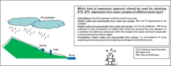
However, we can provide some preliminary recommendations for use of the different regression approaches for the four water types (precipitation, surface water, groundwater from wells, and low-yield springs) from the northern Italian Apennines:
- (i)
In the case of δ18O–δ2H alignments from precipitation, and as no remarkable discrepancies were detected among the several investigated methods, the OLS approach should be preferred.
- (ii)
For precipitation and surface water, slopes and intercepts from the two weighting procedures W and B were similar. Moreover, there was no evidence of remarkable changes among results obtained from such weighting procedures with those from unweighted OLS. The latter confirms the convenience of using the OLS approach even if, during the year, rainfall or discharge amounts (and isotopic content too) are different between the seasons.
- (iii)
For surface water and groundwater, the MA and R approaches should not be used in any case as they seem to provide unrealistic values for both slopes and intercepts. The reason has to be searched in the fact that these two approaches are more sensitive to the statistical performance of the regressions (i.e., standard deviations), especially if outliers are present. MA demonstrated to be more sensitive to the statistical performance of the regressions (i.e., standard deviations), especially if outliers are present. Although the R approach was selected to verify its behaviour in the case of outliers, it did not induce improvements in standardised residuals. Moreover, it was also demonstrated that kinetic fractionation processes acting on these water types lead to increase the differences in slopes and intercepts (see, for instance, relationships between differences in intercepts and slopes with young water fraction Fyw). Slopes and intercepts from OLS and PW were the closest, with lower standard deviations sometimes associated to PW regressions. In addition, and with reference to the surface water, PW results were not affected by the kinetic fractionation processes (see
Table 6 and
Table 7).
- (iv)
Surface water may be affected by nonstationary processes induced by both nonmultivariate normality and serial correlations of the residuals. Thus, prior to carrying out OLS regression on δ18O–δ2H data from surface water (and groundwater), the presences of outliers, heteroscedasticity, and autocorrelation must be carefully detected by means of both conventional statistical tests and inspections of standardised residuals. In the case of outliers, their importance on the whole data series composing the regression should be evaluated (as an instance, in the case of δ18O–δ2H pairs from surface water collected during the late summer through the beginning of the autumn period, the strong reduction in discharges may induce their removal from the dataset prior to carrying out the regression). In the event of dealing with time series of stable isotopes affected by autocorrelation, we believe it is convenient to use the PW approach, which, in our case, has proven to solve the serial correlations of residuals.
6. Conclusions
We presented the comparison of five different regression approaches applied to δ18O–δ2H data from four different water types collected in the northern Italian Apennines. We found that all the tested approaches converged towards similar values of slopes and intercepts for only stable water isotopes from precipitation. Conversely, differences in slopes and intercepts from surface water and groundwater (collected from wells and low-yield springs) were often significant and related to the robustness of the regressions (i.e., standard deviations of the estimates) and their sensitiveness to outliers and autocorrelation. Moreover, and with reference to surface water, we found evidence of a relationship between young water fraction and the magnitudes in differences of slopes and intercepts, suggesting the control of kinetic fractionation processes (mainly related to sublimation acting on snow cover and, secondary, to active pre-infiltrative evaporation and evapotranspiration processes) on such discrepancies. These results allowed us to provide some recommendations for hydrological and hydrogeological studies involving δ18O–δ2H from the abovementioned water types collected in the northern Italian Apennines. Firstly, as no discrepancies were noticed between slopes and intercepts from all the methods applied to precipitation, the OLS approach is preferred. Secondly, and with reference to the other water types (surface water and groundwater from wells and springs), we warmly suggest carrying out conventional statistical tests coupled with inspection of standardised residuals for a preliminary check on the presence of outliers and autocorrelation phenomena. In the case of managing outliers, the MA and R approaches should be avoided as they are more sensitive to the statistical performance of the regressions and often provide unrealistic values of both slopes and intercepts. Thirdly, for surface water and groundwater, the OLS and PW approaches still showed the highest degree of robustness and produced the closest values of slopes and intercepts, thus resulting as the methods preferable for δ18O–δ2H regressions. PW would be more reliable in the presence of serial correlations of the residuals (which, in our case, often affected surface water). In the case of managing outliers, the possibility of removing them will have to be considered (as an example in the case of δ18O–δ2H pairs from marked low-flow periods).
Lastly, despite the presence of marked differences in the amounts of rainfall and their isotopic contents during the year, the convenience of using weighing approaches before applying OLS was not found.


