Article

A Near Real-Time Hydrological Information System for the Upper Danube Basin

Institute for Hydrology and Water Management, University of Natural Resources and Life Sciences, Vienna (BOKU), Muthgasse 18, 1190 Vienna, Austria
*
Author to whom correspondence should be addressed.
Hydrology 2021, 8(4), 144; https://doi.org/10.3390/hydrology8040144
Submission received: 21 July 2021 / Revised: 15 September 2021 / Accepted: 19 September 2021 / Published: 23 September 2021
(This article belongs to the Special Issue Observations in Water Resources)

Abstract

:
The multi-national catchment of the Upper Danube covers an area of more than 100,000 km2 and is of great ecological and economic value. Its hydrological states (e.g., runoff conditions, snow cover states or groundwater levels) affect fresh-water supply, agriculture, hydropower, transport and many other sectors. The timely knowledge of the current status is therefore of importance to decision makers from administration or practice but also the interested public. Therefore, a web-based, near real-time hydrological information system was conceptualized and developed for the Upper Danube upstream of Vienna (Upper Danube HIS), utilizing ERA5 reanalysis data (ERA5) and hydrological simulations provided by the semi-distributed hydrological model COSERO. The ERA5 reanalysis data led to comparatively high simulation performance for a total of 65 subbasins with a median NSE and KGE of 0.69 and 0.81 in the parameter calibration and 0.63 and 0.75 in the validation period. The Upper Danube HIS was implemented within the R programming environment as a web application based on the Shiny framework. This enables an intuitive, interactive access to the system. It offers various capabilities for a hydrometeorological analysis of the 65 subbasins of the Upper Danube basin, inter alia, a method for the identification of hydrometeorological droughts. This proof of concept and system underlines how valuable information can be obtained from freely accessible data and by the means of open source software and is made available to the hydrological community, water managers and the public.

1. Introduction

The way in which environmental information is collected, processed and communicated is changing [1]. The World Wide Web facilitates access to published environmental datasets from remote resources through web-based application programming interfaces (APIs). Geospatial web APIs enable dynamic subsetting, and published datasets give data consumers confidence to access these public sources [1]. The visualization and communication of data and research results are important but at the same time can be challenging. Today, various methods of statistical computing and the graphical visualization of environmental data are open access and feasible by means of free software. However, certain programming skills are still a prerequisite for handling and analyzing geospatial data. Hence, modern methods of statistical and graphical computing are often inaccessible for many researchers [2]. At the same time, advances in data science allow even unexperienced users to interactively explore environmental information [3]. By the use of web-based data visualization techniques, researchers are able to share scientific insight in a way that enables stakeholders to explore the data themselves. These visualization techniques can be especially valuable when data, which cover longer time periods and are spatially distributed, are to be shared. Hydrometeorological datasets can have such characteristics, as they can range over decades, containing millions of observations for several geospatially distributed variables.
Available information systems can offer an opportunity for users without programming skills to explore and visualize hydrometeorological data. “eHYD,” for instance, provides hydrometeorological station data of Austria [4], and “Hydris Online” of the federal state of Salzburg presents data on different hydrometeorological variables [5]. In Germany, the UFZ Drought Monitor offers daily information on drought and soil moisture [6], and the HYPE of the Swedish Meteorological and Hydrological Institute provides information on water quantity and quality on different scales (i.e., world, Europe, Arctic and Niger) [7]. The EU Joint Research Centre (JRC) facilitates the European Flood Awareness System, which utilizes various data sources for hydrological modelling and forecasting [8]. The JRC furthermore developed, together with the European Centre for Medium-Range Weather Forecasts (ECMWF), the Global Flood Awareness System. This system combines weather forecasts with hydrological simulations to provide worldwide flood forecasts [9]. The aforementioned systems are examples of hydrometeorological information systems of different scales covering different regions. These systems produce and distribute valuable hydrological, meteorological and climatical information, and many more are accessible on the Internet (e.g., the US National Oceanic and Atmospheric Administration’s Global Drought Monitor). A hydrological information system (HIS), which focuses on the Upper Danube basin, is in contrast unavailable at the present moment. The Upper Danube basin upstream of Vienna, Austria in Central Europe covers an area of around one hundred thousand square kilometers, with parts in several European countries. Multi-national stakeholders of the Upper Danube and its tributaries depend on topical information on local waterbodies. A hydrological information system for the Upper Danube basin can therefore be a valuable tool for the monitoring of the hydrological states of this diverse and extensive region. It can support researchers in the investigation and visualization of the spatiotemporal interrelationships of different hydrometeorological variables. Water resource and hydropower managers can benefit from a system that offers historical and actual information on the discharge and water levels of local water bodies. Meteorological aggregations and runoff simulations of catchments in the Upper Danube basin can serve as a benchmark for modelers of various fields, e.g., meteorology, climatology or hydrology. Therefore, the aim of the present study is to conceptualize and develop a web-based, near-real-time hydrological information system and thereby provide topical information on the hydrometeorological states of the Upper Danube basin to the hydrological community, water managers and the public.
We present the Upper Danube HIS, which provides various possibilities for the exploration and visualization of hydrometeorological data of the Upper Danube basin, which is available at: https://boku-hywa.shinyapps.io/UpperDanube-HIS/, accessed on 21 September 2021.
The HIS accesses meteorological data from the ERA5 reanalysis data group [10] for simulating runoff in the Upper Danube basin with the conceptual, semi-distributed rainfall-runoff model COSERO [11]. Since the ERA5 data is five days behind present time, the HIS cannot be applied for flood monitoring [12]. On the contrary, droughts commonly develop slower and are even often unnoticed [12], and they can have diverse and severe economic, ecological and societal impacts. Projections of the impact of climate change on the hydrological regime of the Upper Danube basin show a reduced summer runoff, which is most distinct in the Alps [13], and an extended hydrological dry season [14]. Therefore, a 30 day variable threshold [15] was implemented in the Upper Danube HIS, which allows for an identification of the hydrometeorological deficits of different variables, e.g., precipitation, discharge or water stored in the soil reservoir. Besides providing hydrometeorological information on a catchment scale, the HIS furthermore provides real-time hydrological data for Austrian waterbodies. These discharge and water level data are accessed through a Web Feature Service (WFS) of the Central Hydrographical Office of Austria [16].
The paper is organized as follows: Section 2 offers a description of the study area and the utilized data, the preprocessing of the data and the calibration and validation of the COSERO model. Section 3 first describes the calibration and validation of the COSERO model and afterwards focuses on the presentation of the Upper Danube HIS. In this chapter, the implementation of the system, user interface, system capabilities and potential use cases are described. Section 4 provides a discussion of the developed hydrological information system, and Section 5 provides a conclusion.

2. Materials and Methods

2.1. Study Area

The Danube River basin covers a total area of around 801,463 km2 and is, draining (parts of) 19 countries, considered the most international river basin in the world. It is of great ecological, social and economic value, as it provides water supply for industry, agriculture and a variety of eco-systems. The Danube furthermore plays an essential role for transport, power generation, recreation, tourism, fishing and biodiversity [17]. Upstream of Vienna, an area of 102,502 km2, constitutes the basin of the Upper Danube, which is shown in Figure 1. The river originates from a mountain range ‘Schwarzwald’ in southwestern Germany and subsequently travels around 900 km until it reaches Korneuburg, the outlet of the Upper Danube basin, right before Vienna. Besides the main areas of the basin being in Germany and Austria, areas in Switzerland, Italy and the Czech Republic are also within the catchment divide. Two contrary regions dominate the basin area. The northern half predominately consist of low land areas, whereas the mountain range of the Eastern Alps predominates in the south. The elevation ranges from 174 up to 3378 m a.s.l. Due to high elevations and high precipitation sums in the alpine region compared to its northern opponent, the south strongly influences the hydrological regime in the Upper Danube basin. Alpine features such as low winter temperatures, snow accumulation and melt processes especially dominate the runoff characteristics. It has been shown that although the alpine region is solely around 10% of the total area, it is responsible for 26% of the observed discharge of the Upper Danube [18]. The main tributaries in the south of the Upper Danube are from west to east: Lech, Isar, Inn, Salzach, Traun and Enns. The Naab river in the north originates in the Bavarian forest and travels south into the Upper Danube. The land cover in the Upper Danube basin is diverse. However, approximately half of the area is dominated by coniferous forest, meadows and pastures [19]. On the contrary, glaciers and wetlands represent less than one percent. Regarding soil texture distribution in the study area, ‘medium’ texture (i.e., 18% < clay < 35% and sand > 15%) is predominant, with a share of more than 50% in this area. Around the Upper Danube, ‘coarse’ (i.e., clay < 18% and sand > 65%) and ‘medium fine’ (i.e., clay < 35% and sand < 15%) are the dominant texture classes [19].

2.2. Data

Land cover and elevation data were downloaded from the Copernicus Land Monitoring Service [19]. Soil information was retrieved from the soil map of the European Food Safety Authority Data and EU Joint Research Centre [22]. The spatial division of the catchment into subbasins and Hydrological Response Units (HRUs), as well as the discharge data that were used for the parameter calibration of the rainfall-runoff model COSERO, was obtained from the Clim2Power (C2P) project [23]. The numbers in Figure 1 refer to Table A1, which lists all subbasins, the according river and its runoff gauge. Runoff observations were downloaded from the website eHYD of the Central Hydrographical Office of Austria (Hydrographisches Zentralbüro) [4] and from the Bavarian state office for Environment (Gewässerkundlicher Dienst Bayern) [24] for Germany. The discharge dataset of the Upper Danube basin consists of observational data of 54 hydrological gauges. Eleven subbasins are ungauged because the available runoff data were either insufficient or unavailable. A web feature service (WFS) from the hydrographic service is used to retrieve near real-time data of the discharge gauges of Austrian waterbodies since mid-August 2020 [16]. The WFS structure and functionalities comply with the Open Geospatial Consortium (OGC) framework. If an HTTP request is sent to the WFS, information in the Geography Markup Language (GML) data format is returned. The GML data is updated on a half-hourly basis and stores information of hydrological gauges in Austria regarding current water levels, discharge and further information (e.g., gauge name, ID and coordinates). These half-hourly discharge observations are aggregated in order to obtain daily values. A total of 19 gauges from the WFS can be used as observed discharge data for the subbasin gauges of the Upper Danube basin.
The ERA5 data group was used to retrieve the meteorological data of the Upper Danube basin. ERA5 assimilates a large amount of satellite and in-situ data of the near surface and the upper air by atmospheric model, which is coupled with a land surface and a wave model [25] and provides spatially distributed information on several meteorological fields, including temperature and precipitation. It is a world-spanning gridded dataset with a spatial resolution of 31 km and an hourly temporal resolution on 137 levels from the surface up to around 80 km, spanning from 1981 to two to three months before present time [25]. Also being part of the ERA5 data group is the ERA5-Land dataset. The ERA5-Land dataset offers an enhanced spatial resolution of around 9 km and thereby increases the data accuracy for land applications [10]. The data can be requested from the Climate Data Store (CDS) through a web interface, a toolbox or an API [26]. Since the ERA5-Land data is only available until three months before present time, the ERA5 data, which continue to be extended forward near real-time [25], are used to close this three-month gap of ERA5-Land data. Daily updates of the ERA5 data enable a near real-time application of the Upper Danube HIS, and monthly updates of the ERA5-Land data enhance the geospatial resolution and thus provide more accurate meteorological input data for the hydrological modelling procedure. The CDS API is utilized for the daily and monthly data retrieval of the ERA5 and ERA5-Land datasets.

2.3. COSERO Model

Hydrological measurement techniques are limited in space and time. These limitations can be addressed by the extrapolation and prediction from available data through the modeling of hydrological processes [27]. Rainfall-runoff (RR) modelling is widely considered an important tool for water and environment resource management [28]. Its use and advancements of rainfall-runoff models can enhance system and process understanding and improve decision making [27]. The RR model COSERO (Continuous Semi-distributed RunOff) was initially developed for a runoff forecasting model for the Enns river in Austria in the 1990s [29]. Since its development, the COSERO model has continuously been improved. It was applied to assess impacts of climate change on hydrological systems and anthropogenic influence on flooding [28,29]. Various commercial and scientific studies comparing different spatial and temporal scales have proven its robust and versatile applicability (e.g., [11,30,31,32,33,34,35]). Therefore, COSERO was used in this study for the simulation of the runoff in the Upper Danube catchment based on gridded ERA5 and ERA5-Land data. The COSERO model accounts for the accumulation and melting of snow, actual evapotranspiration, soil water storage, separation of runoff in its components surface flow, inter flow and base flow and routing by the use of a cascade of linear and non-linear reservoirs. A schematic representation of COSERO’s structure of reservoirs, states and fluxes, including the relevant model parameters, is shown in Figure A1, and a detailed list of all variables can be found in [11]. Comprehensive and detailed descriptions of the COSERO model can be found in different publications [11,36,37,38].

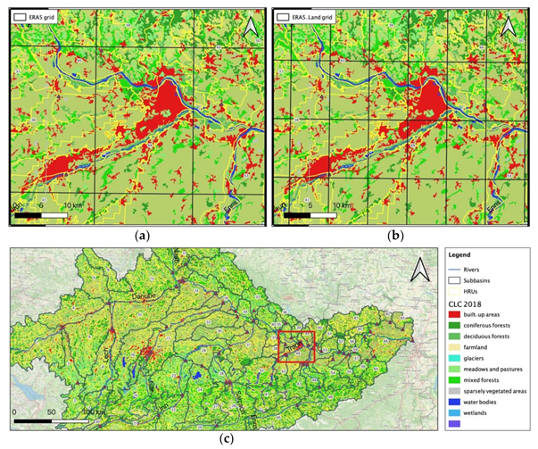
2.3.1. Data Requirements and Preprocessing

COSERO utilizes precipitation, temperature and observed discharge to simulate runoff. Evapotranspiration can optionally be added as input or, as was the case for this study, estimated by temperature after Thornthwaite [11]. COSERO is spatially distributed and therefore all inputs, outputs and model parameters have, besides their time dimension, a spatial dimension. The 65 subbasins of the Upper Danube basin were spatially divided into 3377 HRUs. The model expects meteorological time series for every HRU of the basin. To obtain HRU values for temperature and precipitation, the areal weighted means were calculated by the use of the corresponding data grids. Figure 2 exemplarily shows the ERA5 (a) and ERA5-Land grid (b) for an extent in Upper Austria around the city of Linz. The HRU delineation is indicated in yellow.
Since the ERA5 datasets are either available as hourly or monthly averages and COSERO in the current case is run on a daily timescale, the meteorological inputs precipitation and temperature were aggregated to daily levels in a preprocessing step.

2.3.2. Parameter Calibration and Model Evaluation

Environmental models simulate the response of a system to some input data. Model parameters, initial states and boundary conditions frame the space of possibilities for such modelling exercises. To fit the behavior of system components and their effect on the output, model parameters need to be adjusted to effectively meet each model’s individual purpose [27]. For rainfall-runoff models, system components represent flows (fluxes) and states of reservoirs, and they influence the responsiveness of the model as a whole. The COSERO model has 67 parameters influencing the behavior of the hydrological model. Numerous of these parameters, e.g., elevation or vegetation related parameters, are defined a priori and are therefore not estimated in the process of model calibration. Table A2 lists the resulting 17 model parameters, which were calibrated in the current project, including the parameter ranges used [36]. Generally, very many optimization algorithms exist. Introduced by Bryan Tolson and Christine Shoemaker in 2007, the global optimization algorithm “Dynamically Dimensioned Search” (DDS) is a robust and computationally effective algorithm, offering comparably fast solutions for time demanding optimization problems [37]. Hence, the DDS was applied for automatic parameter calibration of the COSERO model for the Upper Danube catchment. As a limiting factor of the model calibration through the DDS algorithm, the maximum number of iterations was set to 500.
Widely used for the general performance evaluation of hydrological models are the Nash-Sutcliffe efficiency (NSE) [38], the Kling-Gupta efficiency (KG) [39] and the percentage bias (pbias), which is the relative deviation of runoff simulation and observation. Since different study areas can have a different hydrology, the requirements for the measure of goodness of fit can differ [27]. To address runoff characteristics that are specific to the examined catchment, evaluation criteria which focus on different hydrographic features can be used, such as the Peak Difference Coefficient (PDIFF) [35], which focuses on peak discharges, and the logNSE (logarithmic NSE), which focuses on low flows. Further information on the efficiency criteria for hydrological model assessment and a comparison of these can be found in [40].
A model calibration with a single criterion as the objective function can lead to efficient parameterizations and highlight certain properties of a hydrological system [41]. However, if the model calibration solely focuses on one mathematical relation of observations and predictions—hence, a single-criterion optimization—other relevant information of the data might not be represented adequately by the model [42]. Such potential limitations of a single-criterion optimization can be addressed by optimization with multiple criteria. A classical technique for a multi-criteria calibration is the weighted combination of several optimization criteria, where respective weights are defined by users [43]. Since a single-criterion optimization is unlikely to account for all relevant runoff characteristics [44], a multi-criteria optimization was applied in the present study. The multi-criterion optimization was a weighted combination of the model efficiency criteria NSE, logNSE and PDIFF. Shares of the aforementioned evaluation criteria in the objective function were 70% NSE, 20% logNSE and 10% PDIFF. To evaluate the performance of the parameter sets of the multi-criteria optimization, the scores of certain evaluation criteria were examined. These performance indicators were the evaluation criteria NSE, KGE and pbias. The NSE and KGE are dimensionless, whereas the pbias is given in percent.
Meteorological and hydrological time series data from 1982 until 2010 were used for parameter calibration and data from 2008 until May 2017 for respective validation of the model. The first two years of the time series for calibration and validation were used for the spin-up phase of the model, where the system states, e.g., the water content in the soil reservoir, can consolidate sufficiently before the actual calibration or validation phase starts.

2.4. Identification of Hydrometeorological Deficits: Thirty-Days Moving Window Quantile Threshold

The Upper Danube basin is a large area that covers various types of subbasins. Due to this heterogeneity and the alpine character of many southern catchments, the 30D threshold level method is used to identify deficits by means of the HIS. The 30D threshold level can be formulated as shown in Equation (1) [15]:
τ 30 D m = quantile m 14   day   m + 15
The quantiles are calculated from a thirty day window around each day of the year. That means that flow values of 14 days before each day and 15 days after it in all years of the time series constitute the individual distribution of each day of the year. Thereby, each day has an individual threshold level, which results from the quantile of this thirty day long term flow distribution. The 30D variable threshold used by Van Loon and Laaha in their study ‘Hydrological drought severity explained by climate and catchment’ in 2016 was based on the 80th percentile of the flow duration curve of discharge/precipitation of each day [45]. In the present study, the 30D threshold level method is therefore also based on the 80th percentile. This variable threshold method allows for an adaption of low and high flow seasons in Alpine catchments [45] and is implemented in the Upper Danube HIS to support the identification of hydrometeorological deficits.

2.5. Software Implementation

The R programming language is a Free Software, under the terms of the Free Software Foundation’s GNU General Public License, for statistical computing [46]. The programming is object-oriented and functional. R provides a wide range of statistical and graphical data science techniques. It is considered a powerful programming environment for data manipulation, calculation and visualization. Over the last decade, a steep increase in R packages for hydrological sciences has been observed [47]. Several R packages were used for the development of the HIS. The R package ‘ecmwfr’, for instance, is used to gain programmatic access to the CDS in order to retrieve meteorological data from the ERA5 datasets [48]. The ‘Shiny’ package by Winston Chang provides the framework for the developed Upper Danube HIS web-app [49], and the R package ‘lfStat’ is used to calculate the 30 day variable threshold levels [50]. For a complete list of used R packages, see Table A3.

3. Results

First, the performance of the COSERO model with ERA5-Land data in the model calibration and validation period of the multi-criteria optimization is evaluated. Subsequently, the implementation of the hydrological information system, its capabilities and itspotential applications are described.

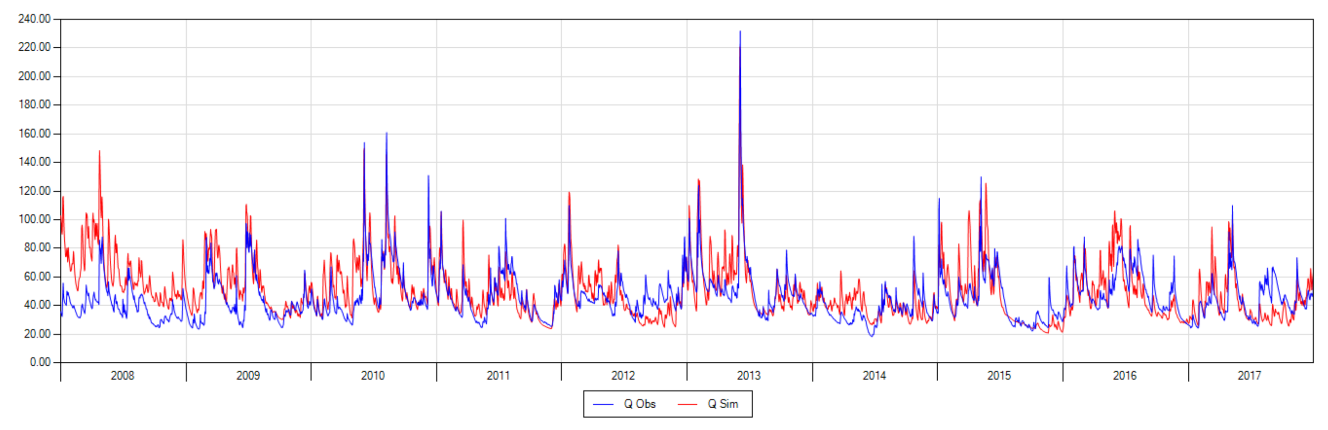
3.1. Calibration and Validation

Table A3 lists resulting evaluation criteria for the multi-criteria optimization for each subbasin. Summary statistics for the listed evaluation criteria are stated at the bottom. In the calibration process, the NSE ranges from a minimum of −0.22 up to 0.83 with a mean of 0.62 and a median of 0.69. The KGE, on the other hand, starts at 0.03 and reaches its maximum at 0.89 with a mean of 0.74 and a median of 0.81. The pbias ranges from −15.56 up to 95.26, with a mean of 13.21 and a median of 9.96. The validation of the parameterization lead to an NSE ranging from −0.56 up to a maximum of 0.79, with a mean of 0.55 and a median of 0.63. The KGE ranges from −0.27 up to 0.88, with a mean of 0.67 and a median of 0.75. The pbias ranges from −44.20 up to 125.03, with a mean of 11.60 and a median of 6.73. The changes of the evaluation criteria from calibration to validation are addressed in the columns ∆ NSE, ∆ KGE and ∆ pbias in Table A3. A negative value in the ∆ column indicates a decrease of the evaluation criteria. For the NSE and KGE, a decrease stands for a loss of predictive power. For the pbias, however, a negative value means a decrease in overestimation or underestimation and therefore an improvement. Both, NSE and KGE show a slight decrease from calibration to validation of −0.08 and −0.07, respectively. Mean pbias stays roughly the same.
Figure 3 shows the spatial distribution of the NSE and KGE scores of the model calibration in the left column and of the validation period in the right column.
Figure 4 shows the cumulative distribution functions (cdf) for the evaluation criteria NSE, KGE, Pearson correlation coefficient (r) and pbias. In each plot, two curves illustrate the cdfs of the respective criterion of the model calibration and validation period of the multi-criteria optimization. A steep function indicates a narrow variance of the distribution. The closer the cdfs of NSE, KGE and r are to 1, the higher the distribution of the evaluation scores. Same goes for the pbias criterion but towards 0%.
In all four plots, the cdfs of the evaluation criteria show similar shapes. The dark cyan curve shows the cumulated frequency of the calibration period whereas the light cyan curve shows the one for the validation. The calibration period yields a superior performance compared to the validation period. The cdfs of the Pearson correlation coefficient of single and multi-objective optimizations are fairly close to each other.

3.2. Upper Danube HIS

3.2.1. Implementation

The Upper Danube basin covers parts of Austria, Germany, Switzerland, Italy and the Czech Republic. The Upper Danube HIS aims to provide an overview on the hydrometeorological conditions for this large area. An operation on the HRU level would result in the handling of 3377 individual spatial units. This would lead to large datafiles and hence slow down the system. The subbasin level offers a reasonable spatial scale for the examination of spatial variability in the Upper Danube basin and is therefore being used.
The Upper Danube HIS is implemented as a sequence of daily and monthly executed R scripts in a specific folder structure on a Windows server. These scripts achieve the required tasks by fetching input data, performing calculations and manipulating data, thereby providing certain outputs, which are further processed (e.g., input datafiles for the COSERO model). A local server is used to request ERA5 and ERA5-Land data from the CDS and hydrological data from the HZB. Table 1 lists the variables that can be visualized in the HIS, including the source of the data.
The HIS preprocesses the retrieved data, runs the COSERO model and updates the web-app with the recent simulations. The web-app can be accessed here: https://boku-hywa.shinyapps.io/UpperDanube-HIS/, accessed on 21 September 2021.

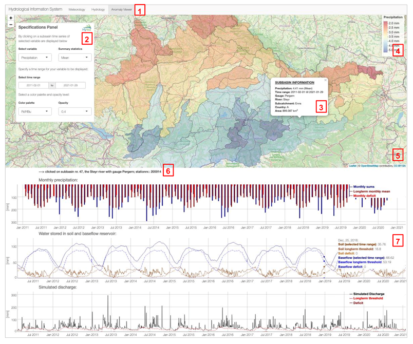
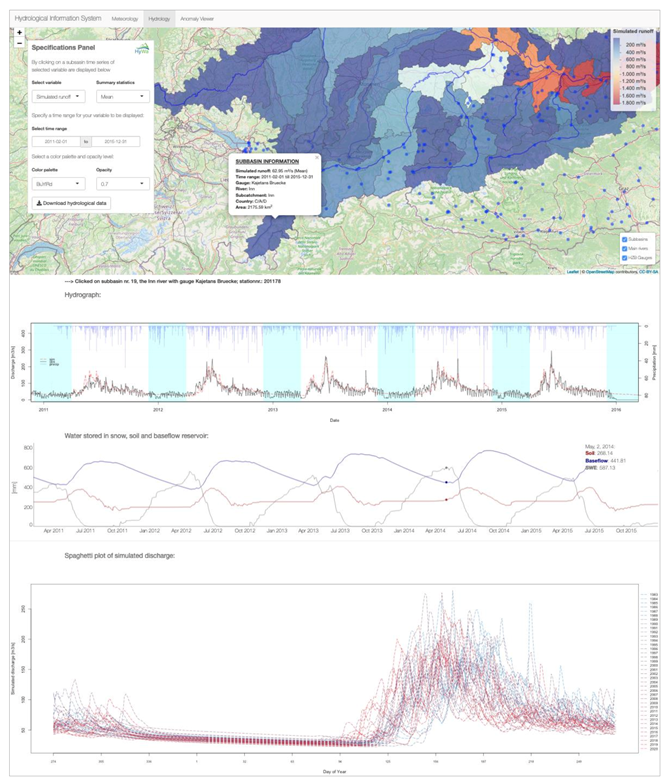
3.2.2. User Interface

The user interface includes three tabs, namely ‘meteorology’, ‘hydrology’ and ‘anomaly viewer,’ which offer information on these three topics. A screenshot of the anomaly viewer tab is shown in Figure 5. The numbers in the parentheses in this subsection refer to the features of the user interface, which are indicated in Figure 5 or in subsequent figures. Figure 5 shows the general structure of the three tabs (1). Each tab shows a map of the Upper Danube basin (5), including a legend for the visualized data (4). The input controls are in the specifications panel (2) on the left side of the map. A pop-up window (3) and a generated text (6) provide further information on the selected subbasin. Depending on the tab, different time series plots (7) are shown below the map. The geospatial visualization of the subbasins and the time series plots depend on the selected input controls. The selection of input controls depends on the respective tab topic.
The meteorology tab provides hydrometeorological information on the subbasins of the Upper Danube region. The variable selection for the map consists of temperature, precipitation, liquid precipitation, solid precipitation, actual evapotranspiration and potential evapotranspiration. Below the map, time series of precipitation, temperature and actual evapotranspiration are plotted.
In the hydrology tab, the observed runoff, the simulated runoff, the water stored in the soil reservoir, the water stored in the baseflow reservoir and the snow water equivalent can be visualized. The plots in the hydrology tab show a hydrograph, containing observed and simulated discharge and precipitation data for the selected subbasin. The second plot shows time series data of COSERO’s system states. These include water stored in the soil reservoir, water stored in the baseflow reservoir and the snow water equivalent. The third and last one are a flow spaghetti plot.
In the anomaly viewer tab, the variables precipitation, water stored in the baseflow reservoir, water stored in the soil reservoir and observed runoff can be visualized. The first plot in this tab shows actual monthly precipitation sums, long-term monthly means and, if occurring, the deficit of the actual monthly precipitation compared to the respective long-term mean value. The middle plot shows time series of the COSERO states ‘water stored in the baseflow reservoir’ and ‘water stored in the soil reservoir,’ whereas the plot at the bottom shows the simulated discharge of the selected subbasin. The middle and the bottom plot show a threshold curve for each variable, which is displayed in the plot.
If the variable undercuts the 30 day window quantile threshold level, a deficit curve is displayed. Figure 6 exemplarily shows the simulated discharge for the years 2017 and 2018 in more detail. The 30 day window quantile threshold, named ‘long-term threshold’ in the legend, is shown as a dashed red line. Additionally, in the legend, the numerical values of simulated discharge, long-term threshold and occurrence are shown. Any day within the selected time range can be examined by maneuvering the cursor along the X axis of the discharge plot. All plots are dynamic and can be zoomed.

3.2.3. System Capabilities

The HIS offers various operations for the analysis of hydrometeorological data in the Upper Danube basin, thereby covering past but also near-real-time periods. The input controls, which determine the specifications of the data and thus the data visualization on the map and by the plots, can be found in the specifications panel on the left side of the map. These input controls are: displayed variable, summary statistics to be shown, time range, color palette and opacity. For the selected time range, the mean, median, minimum or maximum value as well as the sum of the data can be calculated. If input controls are altered, the map and the time series plots are updated accordingly. A pop-up window provides further information with respect to the selected input controls by clicking on a subbasin polygon.
The hydrology map additionally contains the main rivers, the HZB gauges and the impact features layers. The main rivers layer provides information on the corresponding main rivers in headwaters of the Upper Danube, the HZB gauges layer contains additional data of Austrian waterbodies and the impact features layer shows the anthropogenic reservoirs in the Upper Danube basin. This information can be accessed by clicking on a layer feature, as shown for the HZB gauge layer in Figure 7. The pop-up window of a river feature indicates its name and length. The HZB gauge layer displays all hydrological gauges accessed by the WFS. These gauge points display real-time hydrological information of the respective HZB gauge, as the WFS is updated every 15 minutes. Topical information on discharge and water level data can be retrieved from the pop-up window of the HZB gauge. Also shown is the timestamp of the discharge and water level measurement, the name of the gauge and the waterbody and the URL of the corresponding hydrological agency. The impacts layer comprises the main anthropogenic reservoirs in the Upper Danube basin and stems from the LamaH data set [51]. Figure 7 shows the features of the impacts layer around Munich in Germany. By clicking on an impact feature, a pop-up window shows information on the impact type of the feature and, if available, the GRanD (i.e., Global Reservoir and Dam Database [52]) and GOODD (i.e., “global dataset of more than 38,000 georeferenced dams” [53]).

3.2.4. Potential Use Cases

To examine, for instance, the spatiotemporal variability of solid precipitation within the last five years, the respective time range and the maximum statistics could be selected in the specifications panel. Thereby, the spatial distribution of daily solid precipitation and thus the subbasin with the highest daily solid precipitation in this time span can be identified.
If the subbasin with the highest daily solid precipitation is selected, the below time series plots would thus show the temporal patterns of the respective variable (i.e., depending on the selected HIS tab) within the specified time range. Figure 8 shows the visualization of such an inquiry. With the maximum daily solid precipitation of 49.94 mm, the subbasin of the Salzach river with the Bruck gauge yields the highest values in those years. The grey bars in the upper time series plot indicate the solid fraction of the precipitation in the selected subbasin. By the help of the time series plot, the maximum precipitation event can be identified on the 17 November 2019.
For an investigation of hydrological characteristics of the subbasins of the Upper Danube, the hydrology tab can be supportive. Figure 9 shows subbasin 19 (Inn River), with its gauge ‘Kajetan Brücke’ in Tirol. The middle plot indicates that snow is accumulated every season. The SWE goes up to around 540 mm in the examined time range. The hydrograph and the spaghetti plot indicate that the subbasin runoff decreases during winter and increases again with the beginning of the snow melt season, which is a typical characteristic for the alpine catchments.
To investigate the distribution of the water in the soil reservoir, the anomaly viewer tab can be used. Assessing this component of the hydrological cycle can be helpful for examining specific hydrometeorological events, e.g., droughts. Figure 10 shows a screenshot of the anomaly viewer tab with the variable ‘water stored in the soil reservoir’ selected for January 2002 until January 2006. The reoccurring monthly precipitation deficiencies, which can be seen in the monthly precipitation plot as bright red bars, indicate comparably low amounts of water in the soil reservoir of this subbasin. Many other subbasins show a similar shortage in the year of 2003. These deficits can be linked to the drought of 2003 in Central Europe. The HIS can support the assessment of the severity of a drought by providing calculated deficits and visualizing spatial patterns of hydrometeorological variables.

4. Discussion

4.1. Uncertainties

The present study aimed to conceptualize and develop a web-based near-real-time hydrological information system and thereby provide topical information on the hydrometeorological states of the Upper Danube basin to the hydrological community, water managers and the public. However, the HIS, at its present state, has certain limitations. The Upper Danube HIS utilizes reanalysis data from the ERA5 data group. Although the ERA5 datasets can be considered as a high potential alternative for areas of low gauging network densities [54], they are subject to uncertainty. These uncertainties can arise either from the climatological modelling or the assimilated observational data. Furthermore, even the finer ERA5-Land gridded data with around 9 km spatial resolution is beyond the size of the delineated HRUs of the Upper Danube basin since some HRUs are as small as 5 km2. The 31 km spatial resolution of the ERA5 dataset, which is used for the simulation of the last three months until the ERA5-Land dataset is available, even has a coarser resolution. Further potential uncertainties stem from the discharge data. Besides the gap of the discharge data from 2016 to 2020, the acquired real-time data from the HZB gauging system is not verified or corrected by any means. Erroneous discharge observational data does not affect the modelling performance, since the simulations are independent. However, they may influence the information that is being communicated.
Another source of uncertainty can come from the rainfall-runoff model COSERO. Although COSERO is a versatilely applicable hydrological model, especially for European basins with humid climates [34], it is still a model, and all parameter calibration procedures as well as simulations entail uncertainty [27]. Furthermore, several storage hydropower plants exist in the Upper Danube basin. They are not explicitly captured in the hydrological model, which can lead to further uncertainties in the hydrological simulations. Although, the COSERO model achieved satisfactory performance scores (e.g., NSE, KGE, pbias) with the parameter set of the multi-criteria optimization procedure, nine subbasins showed NSE scores lower than 0.5. Figure 11 depicts the location of those subbasins, accompanied by their NSE and KGE score for the calibration period of the model.

4.2. Basins with Poor Simulation Performance

The poor modelling performance of subbasins nr. 15, 16 and 21 can be explained by distinct anthropogenic influences in the gauges’ headwaters, which include reservoirs used for flood mitigation and hydropower plants or diversions. Subbasins nr. 32, 57, 61, 62 and 63 show an overestimation in the discharge simulations, which can be explained by additional groundwater flow that is not being captured by the gauge, too much precipitation input or not enough actual evapotranspiration, all of which are simulated by the model. On the contrary, in subbasin nr. 60, the discharge is underestimated, and the simulated runoff peaks inadequately represent the discharge observations. A detailed examination of the subbasins of poor modelling performance can be found in Appendix B. The value of the hydrometeorological information, provided by the HIS, depends on its quality. It can be argued that provided discharge simulations of poor performance are not a valuable contribution to potential users of the HIS. Therefore, a future advancement of the HIS can be the inclusion of the hydropower reservoirs and operational rules of these (e.g., [55,56]) diversions or the exclusion of subbasins of poor modelling performance.

4.3. Limitations and Future Prospects

Floods can occur in a fast manner, whereas droughts commonly develop slower and even often unnoticed [12]. Nevertheless, droughts can have diverse and severe economic, ecological and societal impacts. An access to a real-time data resource would allow for the implementation of a method for flood detection. Since the ERA5 dataset is five days behind present time, a 30 day moving window threshold was implemented in the Upper Danube HIS. The implementation of this method can support the identification of deficits in the hydrological cycle and the visualization of spatiotemporal interrelationships in the Upper Danube basin.
Other applications or use cases are conceivable with the hydro-meteorological information provided by the HIS. For examples, simulated soil moisture in the HIS is a hydrological field, which can be very useful for hydrogeological risk assessment. Landslide susceptibility is higher during saturated soil conditions. Therefore, knowing this parameter at sub-basin scale can be useful for properly handling precipitation thresholds, which are the basis of landslide activation forecasting and monitoring. Moreover, during the summer, fire susceptibility is also a function of soil humidity content and this parameter is therefore also useful for this kind of risk management.
It should be kept in mind that the system does not provide information on smaller spatial scales than subbasins and smaller temporal scales than days. Furthermore, since no correction method is implemented in the hydrological information system, the hydrological modelling is not being corrected by recent discharge observations. Future advancements of the HIS could address this issue by implementing an according correction method, e.g., through the updating of system states based on information from the discharge observations [57]. It is further noticeable that an automated system also needs maintenance servicing and hence demands supervision.
Currently, the HIS offers information on hydrological states and fluxes. Increasing low flow situations and increasing water temperatures in the rivers also leads to challenges in the operation of thermal power plants. Higher water temperatures of water abstracted for the operation of the power plants lead to a reduction of cooling efficiency on the one hand but can also lead to the violation of legal constraints regarding maximum allowed river temperatures due to ecological reasons. These thresholds may be exceeded when warmed-up water is directed into the river after the power plant [58]. Knowledge of current temperature conditions could therefore help thermal power plant operators to plan accordingly, and the implementation of water temperature simulations in the HIS, e.g., following the methods shown in [58], is feasible for the future.

5. Conclusions

It has been shown how a valuable information system can be conceptualized and implemented with open access hydrometeorological data and free software. The use of modern data visualization techniques has been demonstrated and is being showcased via a web application. Near-real-time runoff simulations are now being updated on a daily basis for 65 subbasins in the Upper Danube basin. This visualization approach enables an interactive exploration and investigation of the hydrological states. Furthermore, it holds potential for the examination of simulations with other data sources and simulations on different spatial and temporal scales. The Upper Danube HIS could also be extended with other hydrological models or other variables, such as water temperature.
Although the HIS and the provided information are subject to some uncertainties and limitations, the calibration and validation of the hydrological model show satisfactory results, and the system offers many capabilities for the investigation of hydrometeorological data. The Upper Danube HIS can be a valuable tool for hydrologists and researchers of related sciences, as well as the interested public. It can furthermore support decision makers like water resources or hydropower managers who rely on actual information on hydrological states in the Upper Danube region, which makes it a valuable contribution for the hydrology community in Central Europe.

Author Contributions

Conceptualization: T.P. and M.H.; methodology: T.P., I.M.S. and M.H.; software: T.P. and M.H.; validation: T.P. and M.H.; formal analysis: T.P.; investigation: T.P. and M.H.; resources: T.P. and K.S.; data curation: T.P. and I.M.S.; writing—original draft preparation: T.P.; writing—review and editing: M.H. and K.S.; visualization: T.P.; supervision: M.H. and K.S.; project administration: M.H. All authors have read and agreed to the published version of the manuscript.

Funding

This research received no external funding.

Data Availability Statement

The study was performed using openly available primary input data. All these input data can be acquired from the rights holders of these data sets. All data and code that were generated in this study are available upon request to the corresponding authors.

Acknowledgments

We thank Christoph Klingler for helping in aggregating ERA5-Land data to HRU scale.

Conflicts of Interest

The authors declare no conflict of interest.

Appendix A

Table A1. Subbasins of the Upper Danube basin.
SubbasinRiverGaugeSubbasinRiverGauge
1DanubeNA34Danube ZEG RP EastAchleiten
2IllerKempten35Kleine MühlObermühl
3IllerNeu-Ulm Bad Held Donau36Grosse MühlTeufelmühle
4DanubeNA37NAKropfmühle
5WörnitzNA38NAFraham
6DanubeDonauwörth39Grosse RodlRottenegg
7LechLechbruck40DanubeLinz
8LechAugsburg Wertach41TraunEbensee
9AltmühlEichstätt42TraunLambach
10DanubeOberndorf43TraunWels-Lichtenegg
11NaabHeitzenhofen44GusenSt. Georgen an der Gusen
12RegenMarienthal45EnnsLiezen (Röthelbrücke)
13DanubeSchwabelweis46EnnsKraftwerk Schönau
14Danube ZEG RP WestPfelling47SteyrPergern
15IsarMuenchen/Isar48EnnsSteyr (Ortskai)
16AmperInkofen49DanubeMauthausen
17IsarPlattling50AistSchwertberg
18Danube ZEG RP MitteHofkirchen51NaarnHaid
19InnKajetans Bruecke52IsperIsperdorf
20InnImst Bahnhof53DanubeYbbs an der Donau
21InnJenbach Rotholz54YbbsGreimpersdorf
22InnOberaudorf55ErlaufNiederndorf
23InnWasserburg56WeitenbachWeitenegg
24AlzAltenmark oh Traun57MelkMatzleinsdorf
25SalzachBruck (Salzach)58PielachHofstetten
26SalzachSalzburg59DanubeKienstock
27SaalachSiezenheim60KremsImbach
28SalzachAch/Burghausen61KampStiefern
29InnBraunau/Simbach KW62SchmidaHollenstein
30RottRuhstorf63GöllersbachObermallebarn
31InnIngling64TraisenWindpassing
32VilsGrafenmuehle65DanubeKorneuburg
33IlzKaltenegg
Figure A1. Schematic representation of the COSERO model structure, including model parameters, system states and fluxes [11].
Hydrology 08 00144 g0a1
Table A2. Subbasins of the Upper Danube basin [11].
Nr.Parameter Lower ConstraintUpper ConstraintDescription
1RAINTRT04Transition temperature above which precipitation is pure rain
2SNOWTRT−22Transition temperature below which precipitation is pure snow
3CTMIN17Minimum snow melt factor on Dec 21
4CTMAX17Maximum snow melt factor on June 21
5NVAR010Variance for distributing new snowfall with a log-normal distribution
6BETA0.110Parameter to compute runoff generation as a function of soil moisture
7H1120Outlet level of reservoir for simulating surface flow
8TAB11200Recession constant for simulating surface flow
9M10500Storage capacity of the soil
10TVS11400Recession constant for simulating percolation from the surface flow module
11TVS211000Recession constant for simulating percolation from the inter flow module
12H2050Outlet level of reservoir for simulating inter flow
13TAB21500Recession constant for simulating inter flow
14TAB31010,000Recession constant for simulating base flow
15TAB40.33Recession constant for simulating routing within a subbasin
16FKFAK0.11Factor to compute ETA from ETP as a function of soil moisture
17KBF100010,000Recession constant for simulating outflow from the soil module with a linear reservoir
Table A3. R packages used in the Upper Danube HIS.
NameDescriptionReference
abindCombine Multidimensional Arrays[59]
data.tableExtension of ‘data.frame’[60]
dygraphsInterface to ‘Dygraphs’ Interactive Time Series Charting Library[61]
ecmwfrThe ecwmfr package: an interface to ECMWF API endpoints[48]
keyringAccess the System Credential Store from R[62]
leafletCreate Interactive Web Maps with the JavaScript ‘Leaflet’ Library[63]
lfstatCalculation of Low Flow Statistics for Daily Stream Flow Data[50]
lubridateDates and Times Made Easy with lubridate[64]
ncdf4Interface to Unidata netCDF (Version 4 or Earlier) Format Data Files[65]
readrRead Rectangular Text Data[66]
rsconnectDeployment Interface for R Markdown Documents and Shiny Applications[67]
sfSimple Features for R: Standardized Support for Spatial Vector Data[68]
shinyWeb Application Framework for R[49]
stringrSimple, Consistent Wrappers for Common String Operations[69]
taskscheduleRSchedule R Scripts and Processes with the Windows Task Scheduler[70]
tidyverseWelcome to the tidyverse[71]
xtseXtensible Time Series[72]
zooS3 Infrastructure for Regular and Irregular Time Series[73]
Table A4. Evaluation criteria of the multi-criteria optimization.
SubbasinRiverGaugeCalibrationValidation∆NSE∆KGE∆pbias
NSEKGEpbiasNSEKGEpbias
2IllerKempten0.730.862.020.610.806.73−0.12−0.064.71
3IllerNeu-Ulm Bad Held 0.760.867.620.690.843.42−0.07−0.02−4.20
6DanubeDonauwörth0.760.8314.490.730.8410.28−0.030.01−4.21
7LechLechbruck0.580.757.660.460.63−1.48−0.12−0.12−6.18
8LechAugsburg Wertach0.670.819.080.510.755.54−0.16−0.06−3.54
9AltmühlEichstätt0.700.8110.520.570.6621.85−0.12−0.1511.33
10DanubeOberndorf0.760.866.210.700.814.94−0.05−0.05−1.27
11NaabHeitzenhofen0.760.857.460.670.835.20−0.09−0.02−2.26
12RegenMarienthal0.740.859.670.690.845.04−0.050.00−4.63
13DanubeSchwabelweis0.790.8610.700.740.828.91−0.05−0.04−1.79
14DanubePfelling0.790.869.960.750.824.75−0.04−0.05−5.21
15IsarMuenchen/Isar0.370.5736.430.470.5821.770.090.01−14.66
16AmperInnkofen0.480.7512.340.500.752.560.030.00−9.78
17IsarPlattling0.550.7911.800.620.750.520.07−0.04−11.28
18DanubeHofkirchen0.760.8511.480.760.834.690.00−0.02−6.79
19InnKajetans Bruecke0.660.7714.560.500.6314.27−0.16−0.14−0.29
20InnImst Bahnhof0.740.7915.460.680.7613.11−0.06−0.03−2.35
21InnJenbach Rotholz0.710.7518.590.720.7617.090.010.01−1.50
22InnOberaudorf0.750.8213.960.650.7614.34−0.10−0.050.38
23InnWasserburg0.740.8215.590.720.8313.74−0.020.01−1.85
24AlzAltenmark Traun0.510.7324.290.350.6923.84−0.16−0.03−0.45
25SalzachBruck(Salzach)0.650.812.550.680.840.890.030.02−1.66
26SalzachSalzburg0.750.870.200.710.81−4.33−0.05−0.064.13
27SaalachSiezenheim0.590.7123.210.570.6920.45−0.02−0.02−2.76
28SalzachAch/Burghausen0.740.863.320.690.825.43−0.06−0.042.11
30RottRuhstorf0.000.0395.26−0.06−0.27125.03−0.05−0.2929.77
31InnIngling0.770.8413.650.770.885.670.010.04−7.98
32VilsGrafenmuehle−0.220.0591.33−0.56−0.22115.24−0.34−0.2723.91
33IlzKaltenegg0.660.82−4.920.660.81−2.64−0.01−0.02−2.28
34DanubeAchleiten0.820.898.940.760.879.27−0.06−0.020.33
35Kleine MühlObermühl0.640.81−6.470.620.75−2.33−0.01−0.05−4.14
36Grosse MühlTeufelmühle0.690.81−7.320.530.72−6.40−0.16−0.10−0.92
39Grosse RodlRottenegg0.750.852.010.530.739.79−0.22−0.127.78
41TraunEbensee0.670.83−2.340.630.78−1.84−0.05−0.04−0.50
42TraunLambach0.760.84−2.020.730.80−1.08−0.03−0.04−0.94
44GusenSt. Georgen Gusen0.650.7025.540.500.6920.55−0.14−0.01−4.99
45EnnsLiezen0.570.6718.810.300.5421.39−0.27−0.132.58
46EnnsKraftwerk Schönau0.700.855.340.560.7410.89−0.14−0.115.55
47SteyrPergern0.650.80−6.270.630.81−0.25−0.020.01−6.02
48EnnsSteyr (Ortskai)0.740.87−0.680.690.844.53−0.05−0.043.85
50AistSchwertberg0.620.6629.500.620.7119.570.000.05−9.93
51NaarnHaid0.670.7322.190.550.6616.71−0.12−0.07−5.48
52IsperIsperdorf0.650.774.840.490.6810.01−0.15−0.095.17
54YbbsGreimpersdorf0.720.80−10.040.770.83−4.020.050.04−6.02
55ErlaufNiederndorf0.700.83−5.100.740.761.130.04−0.07−3.97
56WeitenbachWeitenegg0.570.6911.640.190.5820.42−0.38−0.118.78
57MelkMatzleinsdorf0.250.0491.800.23−0.0297.75−0.02−0.065.95
58PielachHofstetten0.660.72−15.560.640.62−10.02−0.02−0.10−5.54
59DanubeKienstock0.830.8810.360.790.879.52−0.05−0.01−0.84
60KremsImbach0.390.5019.800.110.4211.03−0.27−0.08−8.77
61KampStiefern0.370.4913.930.220.468.58−0.15−0.02−5.35
62SchmidaHollenstein0.250.555.380.130.08−40.34−0.12−0.4734.96
63GöllersbachObermallebarn0.140.539.820.050.07−44.20−0.09−0.4734.38
64TraisenWindpassing0.700.82−2.670.650.682.08−0.05−0.14−0.59
65DanubeKorneuburg0.830.8810.380.780.878.44−0.05−0.01−1.94
Min−0.220.03−15.56−0.56−0.27−44.20−0.38−0.47−14.66
Max0.830.8995.260.790.88125.030.090.0534.96
Mean0.620.7413.210.550.6711.60−0.08−0.070.41
Median0.690.819.960.630.756.73−0.05−0.04−1.79

Appendix B

This section discusses subbasins, which yielded an NSE of lower than 0.5 in the calibration process of the multi-criteria optimization of the COSERO model. Figure A2 depicts the locations of those subbasins. The coloring scheme in the upper left corner indicates the performance of the respective subbasin.
Figure A2. Eastern part of the study area showing the subbasins with an NSE score lower than 0.5 accompanied by the respective KGE score for the calibration period of the model.
Hydrology 08 00144 g0a2
Table A5 summarizes the evaluation scores for the multi-criteria optimization approach. The NSE, KGE and pbias scores are shown for the model calibration and the validation period. On the right side of the table, the changes of evaluation criteria from the calibration to the validation period is shown.
Table A5. Evaluation criteria of subbasins with an NSE lower than 0.5 in the model calibration.
CalibrationValidationDifference
SubbasinNSEKGEpbiasNSEKGEpbias∆NSE∆KGE∆pbias
150.370.5736.430.470.5821.770.090.01−14.66
160.480.7512.340.500.752.560.030.00−9.78
300.000.0395.26−0.06−0.27125.03−0.05−0.2929.77
32−0.220.0591.33−0.56−0.22115.24−0.34−0.2723.91
570.250.0491.800.23−0.0297.75−0.02−0.065.95
600.390.5019.800.110.4211.03−0.27−0.08−8.77
610.370.4913.930.220.468.58−0.15−0.02−5.35
620.250.555.380.130.08−40.34−0.12−0.4734.96
630.140.539.820.050.07−44.20−0.09−0.4734.38
For subbasin 15, the Isar river is the dominant waterbody and is represented by 143 HRUs in the model. The gauge for this subbasin is located in Munich. Several flood risk mitigation measures help to manage water levels. The Sylvensteinspeicher, a large reservoir in the Isar valley with a total capacity of 124.3 hm3, and hydropower plants Achensee and Walchensee (including diversions) constitute distinct anthropogenic influences in the rivers’ headwaters. The resulting impacts on the natural runoff characteristics can partly explain the poor model performance for this subbasin. The hydrograph for the validation period for this subbasin is shown in Figure A3 and illustrates a general overestimation of the discharge. It is interesting that the NSE increases in the validation compared to the calibration period of the model. The pbias decreases as well, which means that the model performs better in the validation phase. The KGE stays roughly the same. From Table A5, it is evident that the simulations overestimate the observations significantly (pbias around 36% in calibration; around 22% in validation period). This means that either the precipitation input is too high, the actual evapotranspiration is too low or the diversions are not accounted for in the model.
Figure A3. Hydrograph in m3/s of the validation period for subbasin 15.
Hydrology 08 00144 g0a3
The Amper is the dominant river in subbasin 16, and the corresponding hydrological gauge of this subbasin is located in Inkofen in Bavaria. The NSE score of this subbasin increases from 0.48 in the calibration to 0.5 in the validation period, whereas the KGE is 0.75 for both periods. Figure A4 shows the hydrograph for the validation period of the multi-criteria optimization. In the year 2008, the simulated discharge overestimates the discharge observations. This offset diminishes during the year 2009 and cannot be recognized in the later years of the period. Several water management measures exist in the Amper rivers’ headwaters, e.g., the reservoir Amperstausee, and the hydropower plants Kranzberg and Haag utilize the Amper’s discharge for power generation. These features influence the natural runoff characteristics and can influence the performance of the model. The offset shown in the hydrograph in the year 2008 could either stem from too much precipitation input or too little actual evapotranspiration in this period.
Subbasin 30 with gauge Ruhstorf at the Rott river and subbasin 32 with gauge Grafenmühle at the Vils river have the lowest model performance, with an NSE of only 0.07 and −0.08, respectively. These subbasins hence also show a very low KGE and the highest overestimation of observed discharge of all subbasins of around 125% and 115%. Figure A5 and Figure A6 show the hydrographs of the validation period. Both hydrographs show that the simulated runoff continuously overestimates the discharge observations. This can be explained by additional groundwater flow, which is not being captured by the gauge, too much precipitation input or not enough actual evapotranspiration in the model.
Figure A4. Hydrograph in m3/s of the validation period for subbasin 16.
Hydrology 08 00144 g0a4
Figure A5. Hydrograph in m3/s of the validation period for subbasin 30.
Hydrology 08 00144 g0a5
Figure A6. Hydrograph in m3/s of the validation period for subbasin 32.
Hydrology 08 00144 g0a6
At the Melk river and the Matzleinsdorf gauge (subbasin 57), discharge is generally overestimated, as is clearly illustrated in the hydrograph in Figure A7. This means that additional groundwater streamflow that is not being detected by the gauge, too much precipitation input or not enough actual evapotranspiration in the model could explain the overestimation in this subbasin.
Figure A7. Hydrograph in m3/s of the validation period for subbasin 57.
Hydrology 08 00144 g0a7
Figure A8 shows the hydrograph for the validation period of subbasin 60. The poor simulation performance for this subbasin with the Imbach gauge at the Krems river can be linked to inadequate representation of simulated runoff peaks in the discharge observations. The model is not able to replicate this behavior, which may be due to spatial heterogeneity in the subbasin. These heterogenic characteristics are not being sufficiently accounted for by the 15 HRUs into which subbasin 60 is segmented. Additionally, high pbias values of around 27% for the single-objective and 20% for the multi-objective optimization in the calibration of the model indicate that either precipitation input is too high or that actual evapotranspiration is too low.
Figure A8. Hydrograph of the validation period for subbasin 60.
Hydrology 08 00144 g0a8
Discharge observations of the gauge Stiefern at the Kamp river (subbasin 61) show a reoccurring dampened hydrograph, as can be seen in Figure A9. This kind of hydrograph can be explained by a number of headwater reservoirs named Kamptalstauseen and respective water management measures in this subbasin. This explains why the model is not able to replicate observational data in a satisfactory manner.
Figure A9. Hydrograph of the validation period for subbasin 61.
Hydrology 08 00144 g0a9
The poor performance of the model in subbasins 62 and 63, with its gauge in Hollenstein on the Schmida river and gauge Obermallebarn in the Göllersbach river, can also be linked to the spatial variability. This area is comparably dry with high evapotranspiration, which explains the relatively low discharge levels and the high pbias (around 41% in subbasin 62 and around 45% in subbasin 63) in the validation period. Furthermore, both subbasins show comparably frequent and high peak discharges, as can be seen in Figure A10 and Figure A11. Such characteristics are deemed to be an intricate modelling challenge. The three HRUs in subbasin 62 and the nine in subbasin 63 that serve as the spatial organizational division seem to be insufficient in these cases.
Figure A10. Hydrograph of the validation period for subbasin 62.
Hydrology 08 00144 g0a10
Figure A11. Hydrograph of the validation period for subbasin 63.
Hydrology 08 00144 g0a11

References

  1. Frew, J.E.; Dozier, J. Environmental Informatics. Annu. Rev. Environ. Resour. 2012, 37, 449–472. [Google Scholar] [CrossRef]
  2. Moraga, P. SpatialEpiApp: A Shiny web application for the analysis of spatial and spatio-temporal disease data. Spat. Spatio-temporal Epidemiol. 2017, 23, 47–57. [Google Scholar] [CrossRef] [Green Version]
  3. Wojciechowski, J.; Hopkins, A.; Upton, R.N. Interactive Pharmacometric Applications Using R and the Shiny Package. CPT: Pharmacometrics Syst. Pharmacol. 2015, 4, 146–159. [Google Scholar] [CrossRef]
  4. BMLRT. eHYD—der Zugang zu Hydrographischen Daten Österreichs. 2020. Available online: https://ehyd.gv.at/ (accessed on 22 December 2020).
  5. Land Salzburg. Hydris Online. 2020. Available online: https://www.salzburg.gv.at/wasser/hydro/#/Fliessgew%C3%A4sser (accessed on 22 December 2020).
  6. Zink, M.; Samaniego, L.; Kumar, R.; Thober, S.; Mai, J.; Schäfer, D.; Marx, A. The German drought monitor. Environ. Res. Lett. 2016, 11, 074002. [Google Scholar] [CrossRef]
  7. SMHI. HypeWeb-Scientific Estimates of Past, Present and Future Water Resources, HypeWeb. 2020. Available online: https://hypeweb.smhi.se/ (accessed on 6 February 2021).
  8. CEMS-a. Copernicus European Emergency System CEMS—European Flood Awareness System EFAS. 2020. Available online: https://www.efas.eu/ (accessed on 6 February 2021).
  9. CEMS-b. Global Flood Awareness System GloFAS—Global Ensemble Streamflow Forecasting and Flood Forecasting. 2020. Available online: https://www.globalfloods.eu/ (accessed on 6 February 2021).
  10. Sabater, J.M. ERA5-Land hourly data from 1981 to present. Copernicus Climate Change Service (C3S) Climate Data Store (CDS). 2019. [Google Scholar] [CrossRef]
  11. Herrnegger, M.; Senoner, T.; Klotz, D.; Wesemann, J.; Nachtnebel, H.; Schulz, K. COSERO—Handbook 2015 Version 2.0; Institute of Water Management, Hydrology and Hydraulic Engineering: Vienna, Austria, 2015. [Google Scholar]
  12. Van Loon, A.F. Hydrological drought explained. Wiley Interdiscip. Rev. Water 2015, 2, 359–392. [Google Scholar] [CrossRef]
  13. Stagl, J.C.; Hattermann, F.F. Impacts of Climate Change on the Hydrological Regime of the Danube River and Its Tributaries Using an Ensemble of Climate Scenarios. Water 2015, 7, 6139–6172. [Google Scholar] [CrossRef]
  14. Coppola, E.; Verdecchia, M.; Giorgi, F.; Colaiuda, V.; Tomassetti, B.; Lombardi, A. Changing hydrological conditions in the Po basin under global warming. Sci. Total Environ. 2014, 493, 1183–1196. [Google Scholar] [CrossRef] [PubMed]
  15. Beyene, B.S.; van Loon, A.F.; van Lanen, H.A.J.; Torfs, P.J.J.F. Investigation of variable threshold level approaches for hydrological drought identification. Hydrol. Earth Syst. Sci. Discuss. 2014, 11, 12765–12797. [Google Scholar] [CrossRef]
  16. BMLRT. Pegel aktuell Web Feature Service; Bundesministerium Landwirtschaft, Regionen und Tourismus: Wien, Austria, 2020. [Google Scholar]
  17. ICPDR. Danube Basin: Facts & Figures. International Commission for the Protection of the Danube River. Available online: https://www.icpdr.org/flowpaper/viewer/default/files/nodes/documents/icpdr_facts_figures.pdf (accessed on 1 December 2020).
  18. Wesemann, J.; Holzmann, H.; Schulz, K.; Herrnegger, M. Behandlung künstlicher Speicher und Überleitungen in der alpinen Niederschlags-Abfluss-Vorhersage. Osterr. Wasser Abfallwirtsch. 2018, 70, 485–496. [Google Scholar] [CrossRef] [Green Version]
  19. Copernicus. Coperenicus (clc2018). Available online: https://land.copernicus.eu/pan-european/corine-land-cover/clc2018 (accessed on 13 April 2019).
  20. OpenStreetMap Foundation. OpenStreetMap. OpenStreetMap. 2017. Available online: https://www.openstreetmap.org/copyright/en (accessed on 7 November 2020).
  21. Eurostat. Dataset—EU Countries. Eurostat—Your Key to European Statistics. Available online: https://ec.europa.eu/eurostat/web/gisco/geodata/reference-data/administrative-units-statistical-units/countries (accessed on 6 November 2020).
  22. EFSA; JRC. Soil Map 15—Topseoil Texture Class. European Food Safety Athority (EFSA) Data and EU Joint Reserach Centre (JRC). 2020. Available online: https://esdac.jrc.ec.europa.eu/content/european-food-safety-authority-efsa-data-persam-software-tool (accessed on 13 April 2019).
  23. Santos, I.M.; Herrnegger, M.; Holzmann, H. Seasonal discharge forecasting for the Upper Danube. J. Hydrol. Reg. Stud. 2021. submitted for publication. [Google Scholar]
  24. GKD, “Abflussdaten Bayern,” Gewässerkundlicher Dienst Bayern. 2020. Available online: https://www.gkd.bayern.de/de/fluesse/abfluss (accessed on 27 December 2020).
  25. Copernicus Climate Change Service (C3S). ERA5: Fifth Generation of ECMWF Atmospheric Reanalyses of the Global Climate. Copernicus Climate Change Service Climate Data Store (CDS). Available online: https://cds.climate.copernicus.eu/cdsapp#!/home (accessed on 29 January 2020).
  26. ECMWF. The family of ERA5 Datasets—Copernicus Knowledge Base—ECMWF Confluence Wiki. 2020. Available online: https://confluence.ecmwf.int/display/CKB/The+family+of+ERA5+datasets (accessed on 28 December 2020).
  27. Beven, K. Rainfall-Runoff Modelling; John Wiley & Sons: Hoboken, NJ, USA, 2012. [Google Scholar]
  28. Dingman, S.L. Physical Hydrology, 3rd ed.; Waveland Press: Long Grove, IL, USA, 2015. [Google Scholar]
  29. Nachtnebel, H.P.; Baumung, S.; Lettl, W. Abflußprognosemodell für das Einzugsgebiet der Enns und der Steyr Report; Institute of Water Management, Hydology and Hydraulic Engineering, University of Natural Resources and Applied Life Sciences: Vienna, Austria, 1993. [Google Scholar]
  30. Nachtnebel, H.P.; Hebenstreit, K.; Diernhofer, W.; Fuchs, W. Auswirkungen von Klimaänderungen auf die Hydrologie alpiner Einzugsgebiete; Österreichische Abfall- und Wasserwirtschaft: Wien, Austria, 1999; Volume 51, pp. 262–275. [Google Scholar]
  31. Stanzel, P.; Nachtnebel, H.P. Mögliche Auswirkungen des Klimawandels auf den Wasserhaushalt und die Wasserkraftnutzung in Österreich. Österr. Wasser Abfallw. 2010, 62, 180–187. [Google Scholar] [CrossRef]
  32. Herrnegger, M.; Nachtnebel, H.-P.; Haiden, T. Evapotranspiration in high alpine catchments—An important part of the water balance! Hydrol. Res. 2012, 43, 460–475. [Google Scholar] [CrossRef] [Green Version]
  33. Wesemann, J.; Herrnegger, M.; Schulz, K. Hydrological modelling in the anthroposphere: Predicting local runoff in a heavily modified high-alpine catchment. J. Mt. Sci. 2018, 15, 921–938. [Google Scholar] [CrossRef] [Green Version]
  34. Kling, H.; Stanzel, P.; Fuchs, M.; Nachtnebel, H.-P. Performance of the COSERO precipitation–runoff model under non-stationary conditions in basins with different climates. Hydrol. Sci. J. 2015, 60, 1374–1393. [Google Scholar] [CrossRef]
  35. Burgholzer, R. Comparison of manual and automatic Parameter Calibration of the R-R-Model COSERO for the Mur catchment. Master’s Thesis, Universität für Bodenkultur, Wien, Austria, 2017. [Google Scholar]
  36. Herrnegger, M.; Klotz, D.; Wesemann, J.; Nachtnebel, H.P.; Schulz, K. RAINFALL-RUNOFF-MODEL COSERO Handbook 2015; Institute for Hydrology and Water Management, University of Applied Life Sciences: Vienna, Austria, 2015. [Google Scholar]
  37. Tolson, B.A.; Shoemaker, C.A. Dynamically dimensioned search algorithm for computationally efficient watershed model calibration. Water Resour. Res. 2007, 43. [Google Scholar] [CrossRef]
  38. Nash, J.; Sutcliffe, J. River flow forecasting through conceptual models part I—A discussion of principles. J. Hydrol. 1970, 10, 282–290. [Google Scholar] [CrossRef]
  39. Gupta, H.; Kling, H.; Yilmaz, K.K.; Martinez, G.F. Decomposition of the mean squared error and NSE performance criteria: Implications for improving hydrological modelling. J. Hydrol. 2009, 377, 80–91. [Google Scholar] [CrossRef] [Green Version]
  40. Krause, P.; Boyle, D.P.; Bäse, F. Comparison of different efficiency criteria for hydrological model assessment. Adv. Geosci. 2005, 5, 89–97. [Google Scholar] [CrossRef] [Green Version]
  41. Duan, Q. Global optimization for watershed model calibration. Calibration Watershed Models 2003, 6, 89–104. [Google Scholar] [CrossRef]
  42. Vrugt, J.A.; Gupta, H.; Bastidas, L.A.; Bouten, W.; Sorooshian, S. Effective and efficient algorithm for multiobjective optimization of hydrologic models. Water Resour. Res. 2003, 39. [Google Scholar] [CrossRef] [Green Version]
  43. Deb, K.; Sundar, J.; Bhaskara, R.N.U.; Chaudhuri, S. Reference Point Based Multi-Objective Optimization Using Evolutionary Algorithms. Int. J. Comput. Intell. Res. 2006, 2. [Google Scholar] [CrossRef]
  44. Yapo, P.O.; Gupta, H.; Sorooshian, S. Multi-objective global optimization for hydrologic models. J. Hydrol. 1998, 204, 83–97. [Google Scholar] [CrossRef] [Green Version]
  45. Van Loon, A.F.; Laaha, G. Hydrological drought severity explained by climate and catchment characteristics. J. Hydrol. 2015, 526, 3–14. [Google Scholar] [CrossRef] [Green Version]
  46. R Core Team. R: A Language and Environment for Statistical Computing; R Foundation for Statistical Computing: Vienna, Austria, 2020. [Google Scholar]
  47. Slater, L.J.; Thirel, G.; Harrigan, S.; Delaigue, O.; Hurley, A.; Khouakhi, A.; Prosdocimi, I.; Vitolo, C.; Smith, K. Using R in hydrology: A review of recent developments and future directions. Hydrol. Earth Syst. Sci. 2019, 23, 2939–2963. [Google Scholar] [CrossRef] [Green Version]
  48. Hufkens, K.; Stauffer, R.; Campitelli, E. The ecwmfr package: An interface to ECMWF API endpoints. Zenodo 2019. [Google Scholar] [CrossRef]
  49. Winston Chang, J.C.; Allaire, J.J.; Xie, Y.; McPherson, J. Shiny: Web Application Framework for R. R Package Version 1.4.0. Available online: https://CRAN.R-project.org/package=shiny (accessed on 22 September 2021).
  50. Koffler, D.; Gauster, T.; Laaha, G. lfstat: Calculation of Low Flow Statistics for Daily Stream Flow Data. 2016. Available online: https://CRAN.R-project.org/package=lfstat (accessed on 22 September 2021).
  51. Klingler, C.; Schulz, K.; Herrnegger, M. LamaH|Large-Sample Data for Hydrology and Environmental Sciences for Central Europe. Earth Syst. Sci. Data Discuss. 2021, 13, 1–46. [Google Scholar] [CrossRef]
  52. Lehner, B.; Liermann, C.R.; Revenga, C.; Vorosmarty, C.J.; Fekete, B.M.; Crouzet, P.; Döll, P.; Endejan, M.; Frenken, K.; Magome, J.; et al. High-resolution mapping of the world’s reservoirs and dams for sustainable river-flow management. Front. Ecol. Environ. 2011, 9, 494–502. [Google Scholar] [CrossRef] [Green Version]
  53. Mulligan, M.; Van Soesbergen, A.; Sáenz, L. GOODD, a global dataset of more than 38,000 georeferenced dams. Sci. Data 2020, 7, 1–8. [Google Scholar] [CrossRef] [Green Version]
  54. Tarek, M.; Brissette, F.P.; Arsenault, R. Evaluation of the ERA5 reanalysis as a potential reference dataset for hydrological modelling over North America. Hydrol. Earth Syst. Sci. 2020, 24, 2527–2544. [Google Scholar] [CrossRef]
  55. Koch, F.; Prasch, M.; Bach, H.; Mauser, W.; Appel, F.; Weber, M. How Will Hydroelectric Power Generation Develop under Climate Change Scenarios? A Case Study in the Upper Danube Basin. Energies 2011, 4, 1508–1541. [Google Scholar] [CrossRef]
  56. Giudici, F.; Anghileri, D.; Castelletti, A.; Burlando, P. Descriptive or normative: How does reservoir operations modeling influence hydrological simulations under climate change? J. Hydrol. 2021, 595, 125996. [Google Scholar] [CrossRef]
  57. Stanzel, P.; Kahl, B.; Haberl, U.; Herrnegger, M.; Nachtnebel, H.P. Continuous hydrological modelling in the context of real time flood forecasting in alpine Danube tributary catchments. IOP Conf. Ser. Earth Environ. Sci. 2008, 4. [Google Scholar] [CrossRef]
  58. Feigl, M.; Lebiedzinski, K.; Herrnegger, M.; Schulz, K. Machine-learning methods for stream water temperature prediction. Hydrol. Earth Syst. Sci. 2021, 25, 2951–2977. [Google Scholar] [CrossRef]
  59. Plate, T.; Heidberger, R. abind: Combine Multidimensional Arrays. 2016. Available online: https://CRAN.R-project.org/package=abind (accessed on 22 September 2021).
  60. Dowle, M.; Srinivasan, A.; Gorecki, J.; Chirico, M.; Stetsenko, P.; Short, T.; Lianoglou, S.; Antonyan, E.; Bonsch, M.; Parsonage, H.; et al. data.table: Extension of “data.frame”. Available online: https://CRAN.R-project.org/package=data.table (accessed on 22 September 2021).
  61. Vanderkam, D.; Allaire, J.; Owen, J.; Gromer, D.; Thieurmel, B. Dygraphs: Interface to “Dygraphs” Interactive Time Series Charting Library. 2018. Available online: https://CRAN.R-project.org/package=dygraphs (accessed on 22 September 2021).
  62. Csárdi, G. Keyring: Access the System Credential Store from R. 2018. Available online: https://CRAN.R-project.org/package=keyring (accessed on 22 September 2021).
  63. Cheng, J.; Karambelkar, B.; Xie, Y. Leaflet: Create Interactive Web Maps with the JavaScript “Leaflet” Library. 2021. Available online: https://CRAN.R-project.org/package=leaflet (accessed on 22 September 2021).
  64. Grolemund, G.; Wickham, H. Dates and Times Made Easy with lubridate. J. Stat. Softw. 2011, 40, 1–25. [Google Scholar]
  65. Pierce, D. ncdf4: Interface to Unidata netCDF (Version 4 or Earlier) Format Data Files. 2021. Available online: https://CRAN.R-project.org/package=ncdf4 (accessed on 22 September 2021).
  66. Wickham, H.; Hester, J.; Francois, R. readr: Read Rectangular Text Data. Available online: https://CRAN.R-project.org/package=readr (accessed on 22 September 2021).
  67. Allaire, J. rsconnect: Deployment Interface for R Markdown Documents and Shiny Applications. 2019. Available online: https://CRAN.R-project.org/package=rsconnect (accessed on 22 September 2021).
  68. Pebesma, E. Simple Features for R: Standardized Support for Spatial Vector Data. R J. 2018, 10, 439–446. [Google Scholar] [CrossRef] [Green Version]
  69. Wickham, H. stringr: Simple, Consistent Wrappers for Common String Operations. Available online: https://CRAN.R-project.org/package=stringr (accessed on 22 September 2021).
  70. Wijffels, J.; Belmans, O. TaskscheduleR: Schedule R Scripts and Processes with the Windows Task Scheduler. 2018. Available online: https://CRAN.R-project.org/package=taskscheduleR (accessed on 22 September 2021).
  71. Wickham, H.; Averick, M.; Bryan, J.; Chang, W.; McGowan, L.; François, R.; Grolemund, G.; Hayes, A.; Henry, L.; Hester, J.; et al. Welcome to the Tidyverse. J. Open Source Softw. 2019, 4, 1686. [Google Scholar] [CrossRef]
  72. Ryan, J.A.; Ulrich, J.M. xts: eXtensible Time Series. 2020. Available online: https://CRAN.R-project.org/package=xts (accessed on 22 September 2021).
  73. Zeileis, A.; Grothendieck, G. Zoo: S3Infrastructure for Regular and Irregular Time Series. J. Stat. Softw. 2005, 14, 1–27. [Google Scholar] [CrossRef] [Green Version]
Figure 1. The Upper Danube basin in Central Europe. The map shows the main rivers and elevation levels of the basin. The numbers refer to the delineated subbasins (The base map in all maps were obtained from the OpenStreetMap Foundation (© OpenStreetMap contributors, [20]), The EU country vector dataset in all maps were obtained from Eurostat [21]).
Hydrology 08 00144 g001
Figure 2. Spatial distribution of CORINE Land Cover classes in the Upper Danube catchment with ERA5 and ERA5-Land grids in the area of the city of Linz: (a) ERA5, 31 × 31 km2 grid; (b) ERA5-Land, 9 × 9 km2 grid; (c) Overview map showing the location of the extent of (a,b).
Hydrology 08 00144 g002
Figure 3. Comparison of NSE and KGE distribution for the model calibration and validation period of the multi-criteria optimization: (a) NSE distribution of the model calibration; (b) NSE distribution of the validation period; (c) KGE distribution of the model calibration; (d) KGE distribution of the validation period. Detailed numerical values for all subbasins can be found in the Appendix A.
Hydrology 08 00144 g003
Figure 4. Cumulative distribution functions of NSE, KGE, Pearson correlation coefficient and pbias in the model calibration (dark cyan) and validation period (light cyan).
Hydrology 08 00144 g004
Figure 5. A screenshot showing the general structure of the tabs of the Upper Danube HIS by the example of the anomaly viewer Table The top part consists of the data visualization map and the specifications panel. Time series diagrams below the map show the plotted data of different variables for the selected time range. Note that the time series panels are interactive and dynamic, providing seamless zooming capability.
Hydrology 08 00144 g005
Figure 6. Simulated discharge for the years 2017 and 2018. The daily levels of the simulated discharge, the long-term threshold and the discharge deficit are displayed in the legend for a date in July 2017. Exemplary discharge day deficit by a 30 day window quantile threshold level.
Hydrology 08 00144 g006
Figure 7. Examples of pop-up windows of the ancillary layers of the hydrology tab: (a) Provided information of the HZB gauges layer comprises the timestamp of the measured data, the name of the waterbody and hydrological gauge, the discharge and water level and the URL of this correscheme; (b) Provided information of the impact feature laser comprises of impact type, GRanD and GOODD ID.
Hydrology 08 00144 g007
Figure 8. A screenshot showing the spatial distribution of the maximum solid precipitation in the recent five years in the meteorology Table The subbasin with the gauge in Bruck shows the highest daily solid precipitation level and was therefore selected. The below time series plots show liquid and solid precipitation, temperature and actual evapotranspiration for the selected subbasin. The maximum daily solid precipitation is hence shown in the precipitation time series plot. Temperature and actual evapotranspiration data are accompanied by their long-term means.
Hydrology 08 00144 g008
Figure 9. A screenshot showing the hydrology tab with subbasin nr. 19 selected. The data visualization map shows the means of the simulated discharge from February 2011 to January 2016. Selected is subbasin 19 (Inn River), with its gauge ‘Kajetan Brücke’ in Tirol. Below the map, a hydrograph, a time series plot of the variables ‘water stored in the soil reservoir,’ ‘water stored in the baseflow reservoir’ and ‘Snow Water Equivalent,’ along with a Spaghetti plot of the simulated discharge, are shown.
Hydrology 08 00144 g009
Figure 10. A screenshot of the anomaly viewer tab showing information on subbasin nr. 12. The data visualization map shows the spatial distribution of the mean values of the variable ‘water stored in soil reservoir.’ In the below time series plots, information on monthly precipitation, the variables ‘water stored in the soil reservoir’ and ‘water stored in the baseflow reservoir’ and simulated discharge are shown.
Hydrology 08 00144 g010
Figure 11. A map of the Upper Danube basin showing the subbasins with an NSE score lower than 0.5 accompanied by the respective KGE score for the calibration period of the model.
Hydrology 08 00144 g011
Table 1. Variables of the Upper Danube HIS, including their data source.
VariableData Source
TemperatureERA5/ERA5-Land
PrecipitationERA5/ERA5-Land
Liquid precipitationCOSERO
Solid precipitationCOSERO
Actual evapotranspirationCOSERO
Potential evapotranspirationCOSERO
Observed runoffHydrological Services (HZB, GKD)
Simulated runoffCOSERO
Water stored in soil reservoirCOSERO
Water stored in baseflow reservoirCOSERO
Snow water equivalentCOSERO
Publisher’s Note: MDPI stays neutral with regard to jurisdictional claims in published maps and institutional affiliations.

