Article

A Multilayer Perceptron Model for Stochastic Synthesis

Institute for Environmental Research & Sustainable Development, National Observatory of Athens, 15236 Athens, Greece
*
Author to whom correspondence should be addressed.
Hydrology 2021, 8(2), 67; https://doi.org/10.3390/hydrology8020067
Submission received: 27 March 2021 / Revised: 14 April 2021 / Accepted: 16 April 2021 / Published: 19 April 2021

Abstract

:
Time series analysis is a major mathematical tool in hydrology, with the moving average being the most popular model type for this purpose due to its simplicity. During the last 20 years, various studies have focused on an important statistical characteristic, namely the long-term persistence and the simultaneous statistical consistency at all timescales, when different timescales are involved in the simulation. Though these issues have been successfully addressed by various researchers, the solutions that have been suggested are mathematically advanced, which poses a challenge regarding their adoption by practitioners. In this study, a multilayer perceptron network is used to obtain synthetic daily values of rainfall. In order to develop this model, first, an appropriate set of features was selected, and then, a custom cost function was crafted to preserve the important statistical properties in the synthetic time series. This approach was applied to two locations of different climatic conditions that have a long record of daily measurements (more than 100 years for the first and more than 40 years for the second). The results indicate that the suggested methodology is capable of preserving all important statistical characteristics. The advantage of this model is that, once it has been trained, it is straightforward to apply and can be modified easily to analyze other types of hydrologic time series.

1. Introduction

Stochastic models first appeared in hydrology in the early 1950s in the 1954 work of Barnes [1], who generated a 1000-year sequence of mutually independent synthetic annual inflows to design a reservoir on the Upper Yarra river in Australia. Later, Thomas and Fiering [2] introduced the first stochastic model that was capable of reproducing some characteristics of the statistical properties of the natural process. Over the years, various stochastic techniques appeared, with the most popular being the autoregressive models (AR), the moving average models (MA), and their combination (ARMA), which are also known as Box-Jenkins models [3].
Since the introduction of the stochastic models, and after extensive research in this scientific area, various challenges have been highlighted. For example, the magnitude of the autocovariance of the generated time series decays exponentially unless specific techniques are employed [4]. Another challenge is when the time window of the studied hydrologic process extends over different timescales, e.g., generating daily rainfall time series with a length of hundreds of years. In this case, a single model cannot simultaneously focus on the stochastic properties at multiple scales [5].
To cope with these issues, various researchers have suggested approaches that preserve the Hurst coefficient [6] and the autocovariance structure of all time scales with a minimal number of parameters [4]. This statistical property is very important in water management applications because it is related to “the tendency of wet years to cluster into multi-year wet periods or of dry years to cluster into multi-year drought periods” [7]. Furthermore, the stochastic modeling of long time series extending over multiple scales, has been dealt with by utilizing coupling of stochastic models of different time scales [5]. A series of iterations is performed in order to “synchronize” the lower-level and the higher-level models (i.e., achieve a statistical consistency between these two timescales). This approach requires advanced mathematical frameworks and, hence, specialized tools [8,9].
Other models go one step further by incorporating spatially distributed data obtained by either remote sensing devices (e.g., weather radar and satellites) [10] or from general circulation models [11] or earth system models [12]. These two-dimensional weather generators follow a multi-stage approach to blend the higher-scale information into the lower scale. The stages include the spatial downscaling of the input data and then the temporal downscaling with a stochastic model (by adjusting the model parameters according to the predicted changes from large-scale climate model), and finally, the restoration of the statistical dependencies including the inter-annual variability regarding the long-term trends.
Hydrologic approaches based on rigorous mathematical frameworks are important because they help to obtain insight into the complicated properties of the hydrologic processes. On the other hand, various studies have suggested that black-box approaches, like machine learning, can be used in hydrological applications as more straightforward methods [13]. For example, Shuang and Zhao have used various machine learning approaches (MLP network, AdaBoost, Gradient Boosting Decision Tree) to obtain a prediction of the water demand [14]; Rozos has employed an MLP network to optimally manage a complex water supply system [15]; Shin et al. [16] used a Long Short-Term Memory (LSTM) network to evaluate the impact of the groundwater withdrawal on the groundwater level; Niaghi et al. [17] tested various machine learning approaches regarding their efficiency to estimate the reference evapotranspiration; and Minns and Hall [18] used a feedforward network in rainfall-runoff modeling.
The reason for the popularity of the machine learning methods is their conceptual simplicity and their broad scope of application, along with standardized methodology. Though there are plenty of machine learning applications in time-series analysis, most of them are employed at short-term forecasting or surrogate modeling. There are barely any applications in generating synthetic time series. For example, Campos et al. [19] used a neural network to generate synthetic time series of monthly reservoir inflows that is equivalent to an AR(1) model.
In this study, we are proposing the use of a multilayer perceptron (MLP) network [20] for stochastic synthesis of daily rainfall time series. This MLP-based approach is novel because, in contrast to the existing similar approaches, it reproduces the statistical properties of the corresponding historical time series at multiple scales (Hurst effect). We call this model MLPS. We chose MLP, a half-century-old approach, instead of a more recent type of deep learning network for two reasons. First, we found MLP to be sufficiently powerful despite being parsimonious (only a few dozen parameters). In contrast, the deep learning networks tend to employ a much larger set of parameters, from hundreds up to millions (e.g., AlexNet). Second, our motivation is to provide a stochastic model that is fairly simple to implement, even in a spreadsheet [21], a tool with which practitioners, and stakeholders in general, are familiar so that the proposed method has good chances of being adopted by this important community.

2. Materials and Methods

2.1. MLPS

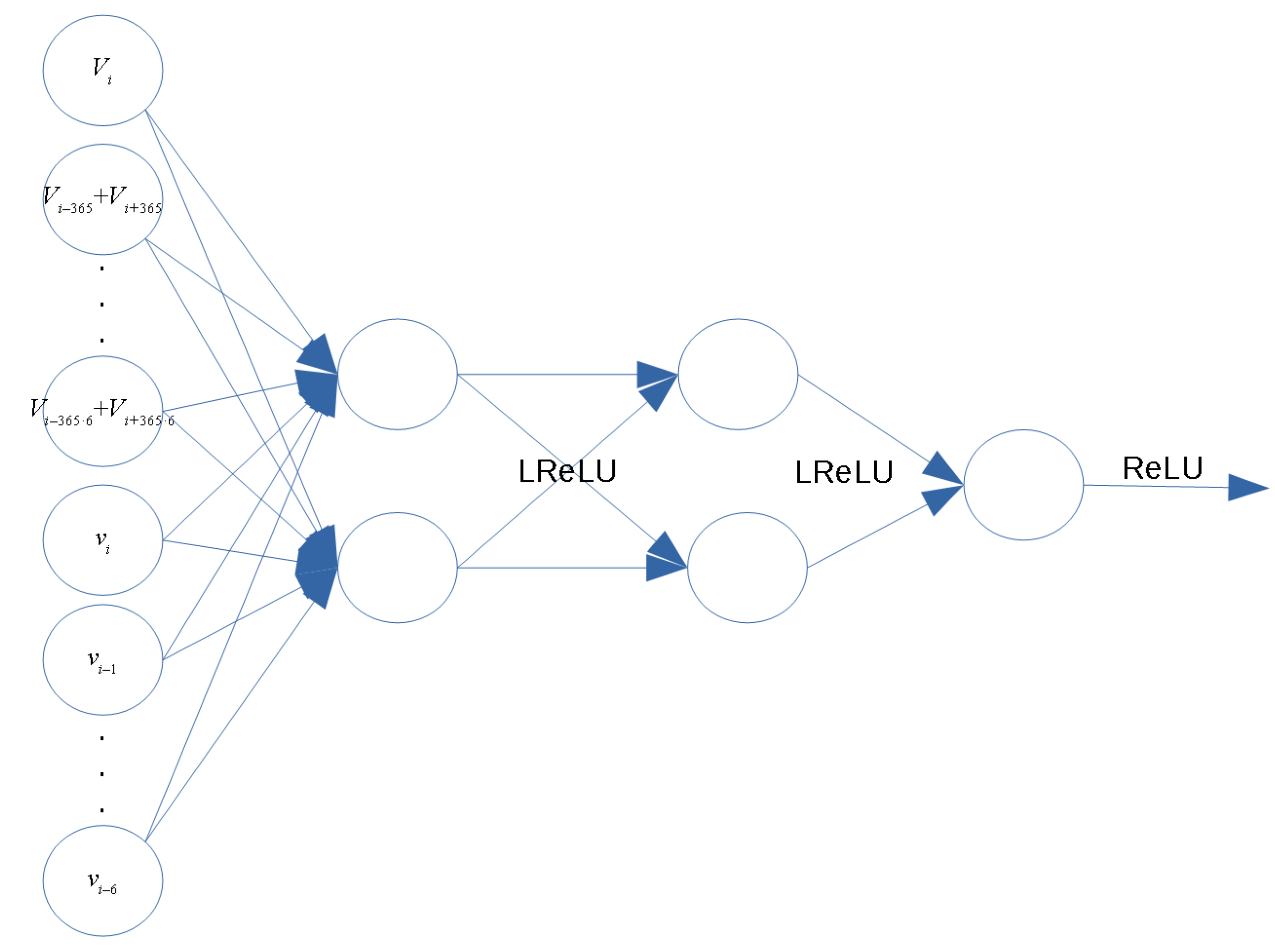
2.1.1. Input Features

The generation of features (i.e., the inputs to the network) is based on formulas (Equation (1) below, and a random number generator) with cyclostationary parameters (e.g., a different parameter value for each month of the year). Therefore, the dates of the synthetic time series should be defined before anything else. The MS Excel date format was used [22] to represent the dates (see Appendix A). For handling the dates, an appropriate function [23] was used to decode a serial number to the corresponding month (used for generating cyclostationary signals) and year (used for aggregating up to annual scale).
The input features were selected to mimic the practices of the previous relevant studies. For example, a symmetric moving average for the annual independent and identically distributed innovations (IIDIs) was used, following Koutsoyiannis’ study, [4], whereas, inspired by the Chen et al.’s study [24,25], a first-order Markov chain in the generation of daily IIDI was employed.
The daily IIDIs were generated employing a method similar to that used by Richardson and Wright [26]. Initially, a first-order two-state Markov chain was used to generate the occurrence of wet or dry days with the following equation:
s i = ( s i 1 1 P 11 m > θ i ) ( s i 1 0 P 01 m > θ i )
where s i is the state of the day i (1 for rainy, 0 for non-rainy); P 11 m (estimated from the historical daily time series) is the probability of the day i of month m of the year ( m = 1 , , 12 ) being wet if the day i 1 is wet; P 01 m is the probability of the day i of month m being wet if the day i 1 is dry; θ i is a random number following uniform distribution.
Then, random numbers v i following a two-parameter Gamma distribution were generated. Different Gamma parameter values were employed for each month of the year (cyclostationarity). To estimate the parameters of the Gamma distribution for the month m, a Nelder-Mead simplex algorithm [27] was employed to minimize the distance between the distributions F ^ m and Γ ( α m , β m ) , where F ^ m is the empirical distribution of the daily non-zero depths of all historical rainfall values of month m and Γ ( α m , β m ) is the Gamma distribution with the optimized parameters α m and β m .
Finally, the daily IIDIs were obtained with the z-score normalization [28]
v i = ( s i v i ) μ v σ v
where μ v and σ v are the mean and the standard deviation of the time series s i v i .
The annual IIDIs, V i , were generated employing also a two-parameter Gamma distribution. The two parameters (a single set, no cyclostationarity) were obtained, like previously, with a fitting procedure employing a Nelder–Mead simplex algorithm. These annual values were initially disaggregated to the daily scale (the time step of the stochastic model), keeping the same value for each day belonging to the same year; then, a moving average was applied with a window of 365 days to smooth out the time series. Note that this smoothing does not induce a central limit theorem effect, because at each summation of the moving average, the 365 values are repetitions of only 2 unique random values (corresponding to two consecutive years). After applying z-score normalization to the smoothed time series, the annual IIDIs were obtained.
After obtaining v i and V i , the features were assembled into a matrix of 14 columns, of which each row F i is given by the following equation.
F i = V i ( V i 365 · 1 + V i + 365 · 1 ) ( V i 365 · 6 + V i + 365 · 6 ) v i v i 1 v i 6

2.1.2. Topology

The optimum topology of the network was found to be 2-2-1 (i.e., two hidden layers). This topology, for 14 inputs, introduces 39 parameters, i.e., 34 weights and 5 biases. The activation function for the last layer was ReLU, whereas LReLU was used for the remaining layers [29]. ReLU is ideal for this application, because it not only facilitates the faster training of the network but also ensures the non-negative values for precipitation. LReLU was used for the other two layers to avoid the ’dying ReLU’ problem [29]. The topology of the network is displayed in Figure 1.

2.1.3. Cost Function

The performance of a network, i.e., the average difference between the actual y i and the simulated values y ^ i , is measured with the cost function [30]. The most typical cost function is the Mean Squared Error (MSE), which for the vector x , containing the weights and biases of the network is given by Equation (4).
C ( x ) = i = 1 n ( y i y ^ i ( x ) ) 2
Besides MSE, there are plenty of alternative cost functions (e.g., MAE, Entropy Loss, Divergence Loss, etc., [31]). All of these have one thing in common: they penalize the deviation of the simulated values from the target values (the historical values in our case). It becomes evident that such a kind of cost function is not suitable for MLPS because the objective is to preserve the statistical structure, not to fit the output to the historical values.
After many experiments, the objective function was fixed on Equation (5), in which 16 metrics (referred to as scalar function D ( , ) ) were combined to obtain a single value.
C ( x ) = W 1 W 16 · D ( [ n 1 S i n 1 S ] i = 1 k 1 , [ n 1 H i n 1 H ] i = 1 k 1 ) D ( n 1 S k 1 n 1 S , n 1 H k 1 n 1 H ) D ( [ n 2 S i n 2 S ] i = 1 k 2 , [ n 2 H i n 2 H ] i = 1 k 2 ) D ( n 2 S k 2 n 2 S , n 2 H k 2 n 2 H ) D ( [ n 3 S i n 3 S ] i = 1 k 3 , [ n 3 H i n 3 H ] i = 1 k 3 ) D ( [ n 4 S i n 4 S ] i = 1 k 4 , [ n 4 H i n 4 H ] i = 1 k 4 ) D ( n 4 S k 4 n 4 S , n 4 H k 4 n 4 H ) D ( [ ρ S l ] l = 1 l max , [ ρ H l ] l = 1 l max ) D ( σ 365 S , σ 365 H ) D ( [ σ 12 S i ] i = 1 12 , [ σ 12 H i ] i = 1 12 ) D ( [ μ 12 S i ] i = 1 12 , [ μ 12 H i ] i = 1 12 ) D ( r S , r H ) D ( μ ˜ 4 S , μ ˜ 4 H ) D ( μ ˜ 3 S , μ ˜ 3 H ) D ( σ S , σ H ) D ( μ S , μ H )
where x is the vector containing the weights and biases of the MLPS network; [ W 1 W 16 ] are the weights of the 16 metrics, which, after numerous trials, were fixed to the values [ 2 , 2 , 2 , 2 , 2 , 2 , 2 , 4 , 10 , 10 , 10 , 10 , 10 , 10 , 10 , 100 ] ; D ( , ) is given in Equation (6); n 1 S i is the number of the sample values lying within the i-th interval (i.e., the histogram; see [32], Equation (5.1)) of the event duration of the synthetic time series (subscript ’S’ is for synthetic) obtained by the MLPS network when run with the values of weights and biases of x ; n 1 S = i = 1 k 1 n 1 S i ; k 1 is the number of intervals into which the space of the event duration is discretized (the same discretization of space is used for both historical and synthetic time series); the following six metrics, with the indexes 2, 3, 4, refer to the dry spell duration, annual rainfall depth, and daily rainfall depth, respectively; ρ S l is the l-lag auto-correlation of the aggregated to annual scale synthetic time series; σ 365 S is the standard deviation of the annual values of the synthetic time series; σ 12 S i is the standard deviation of the synthetic time series values of the ith month of the year; μ 12 S i is the mean value of the synthetic time series values of the ith month of year; r S is the lag-1 auto-correlation of the daily synthetic time series; μ ˜ 4 S is the kurtosis of the daily synthetic time series; μ ˜ 3 S is the skewness of the daily synthetic time series; σ S and μ S are the standard deviation and the mean value of the daily synthetic time series, respectively. Please note that for the typesetting, the IAHS guidelines [33] are followed to improve the clarity of the employed symbols. That is, textual subscripts are in upright (Roman) font. For example, the textual subscripts S and H correspond to synthetic and historical time series, respectively. Therefore, the definitions of the corresponding variables for historical (subscript ’H’) time series can be easily derived from the previous ones.
D ( a , b ) = mean ( [ d ( a i , b i ) ] i = 1 , n )
where a , b are vectors of size n and d ( a , b ) = | a b | / max ( min ( | b | , | a | ) , δ ) . The tolerance coefficient δ (a kind of measure of the significance of the decimal precision) is used to avoid awarding large penalty values to deviations of minor significance. For example, suppose the mean value of the wet month is 5 mm/day and the mean value of the dry is 0.05 mm/day; then, a 0.1 mm/day output from the stochastic model for the dry month is considered satisfactory. Adopting a δ value equal to 0.1 allows to give to this model output a penalty of only 0.5 instead of 1.0 without using δ . Equation (6) is actually the mean absolute error, which gives more weight to the agreement between the average rather than the peaks of the compared values [34].
The value of l m a x in Equation (5) is selected after a preliminary analysis of the historical time series to include all significant ρ H l values.
Note that, (i) in the metrics 1, 3, 5, and 6, the relative number of samples of the historical time series that are 0 are not taken into account in D ( , ) . These 0 values, appearing as gaps in the middle of the histogram of the historical values, are considered artifacts. (ii) The second, forth, and seventh metrics introduce an extra penalty to the failure of preserving the frequency of the most extreme value.

2.1.4. Training

The MLPS network training was accomplished with Genetic Algorithms (GA) [35] instead of the standard backpropagation approach [36]. GA is much slower than any optimization method based on backpropagation. However, the latter is based on the chain rule (e.g., see [30]), which cannot be applied, since there is no closed-form expression of the derivative of Equation (5) with respect to the MLPS network output.
The parameters of the GA were as follows: population size 200, maximum number of generations 800, crossover fraction 0.8, Scattered crossover faction, Gaussian mutation function, elite count 2, scale and shrink both equal to 1. At each generation, 200 ( 1 0.8 ) 2 individuals were mutated. The initial population followed a uniform distribution with values from −10 to 10 (note that GA is not that sensitive to the values of the initial population like gradient-based methods, which suffer from the problem of exploding/vanishing gradients [37]).
To ensure that the network generalizes well, the training was performed with synthetic time series of significant length. For example, this length (actually the maximum value of index i in Equation (3)) was 360,000 days in both case studies presented below.
During the training, bootstrapping was employed [38]. According to this technique, a different subset of the features was used at each cost function evaluation. This subset should be continuous corresponding to consecutive days. The size of the subset was 20% of the length of the features. This technique not only reduces the computational time (since the metrics of Equation (5) are applied on shorter time series) but also helps to improve the model generalization [39].
MLPS was implemented in MATLAB language. GNU Octave (MATLAB open source equivalent) was used in this study to run MLPS. A GA implementation that supports parallel computing [40] was used to accelerate the model training. MLPS was run on a virtual server with eight cores [41].

2.2. WeaGETS

WeaGETS [24] was used as a reference model to evaluate MLPS performance. WeaGETS is a single-site stochastic weather generator (Tmin, Tmax, and rainfall). At the daily time step, first-order Markov chain is employed to switch between dry and wet days. The rainfall depth of the days that are deemed wet is obtained with a random number generator (alternative distributions are available). Then, to account for the low-frequency variability, the daily rainfall depth is corrected using power spectra of the observed time series at monthly and yearly scales. A method similar to coupling of stochastic models suggested by Koutsoyiannis [5] was also employed. The parameters used in WeaGETS were the following:
0.1Daily precipitation threshold
700Number of years to generate
NoSmooth the parameters of precipitation occurrence and quantity
1Order of Markov Chain to generate precipitation occurrence
Skewed normalDistribution to generate wet day precipitation amount
UnconditionalScheme to generate maximum and minimum temperatures
NoCorrect the low-frequency variability of precipitation
It should be noted that MLPS is not compared against WeaGETS in terms of performance superiority. MLPS’s advantage is its conceptual simplicity and straightforward applicability and not any improvement in performance against established models. In fact, WeaGETS was intentionally handicapped by turning off the correction of the low-frequency variability of precipitation. The motive for this was to demonstrate the significance of the long-term persistence effect in time-series analysis.

3. Results

3.1. Application to Hohenpeissenberg

The historical rainfall time series measured at the Hohenpeissenberg Observatory was obtained from Deutscher Wetterdienst. The climate of this location is oceanic (Köppen: Cfb), affected by altitude and proximity to the Alps. The time series starts on the 1 January 1879 and ends on 31 October 2020.
The comparison of the overall statistics of the synthetic time series and historical time series obtained from the weather station of Hohenpeissenberg is given in Table 1. Both models preserved all statistical characteristics well, with the exception of the auto-correlation with 1-day lag of the time series of WeaGETS.
Figure 2 and Figure 3 display the monthly mean and standard deviation of the synthetic and historical values of the Hohenpeissenberg weather station. According to these figures, both models satisfactorily preserved the monthly mean value and the standard deviation.
Figure 4 displays the histogram of the daily time series of the synthetic and historical values. To properly interpret this plot, it should be kept in mind that the longer the bar above the horizontal axis, the higher the frequency, whereas the longer the bar below the horizontal axis, the lower the frequency. For example, the long bars at depths greater than 100 mm correspond to frequency values very close to 0 (no bar is plotted for the values that are equal to 0). According to this figure, both models performed very well.
Figure 5 displays the histogram of the annual (aggregated from daily time step with plain summation) synthetic and historical time series.
Figure 6 displays the histogram of the rainfall events’ duration. Both models performed relatively well. Figure 7 displays the histogram of the duration of dry spells. According to this figure, WeaGETS underestimates the frequency of the dry spells with long duration.
Figure 8 displays the climacogram [42] of the Hohenpeissenberg time series. MLPS fits very well to the marks of the historical time series.

3.2. Application to Gibraltar

The historical rainfall time series measured at the Gibraltar meteorologic station was obtained from freemteo.org. The climate of this location is Mediterranean (Köppen: Csa). The time series starts on the 1 January 1974 and ends on the 29 December 2015.
The comparison of the overall statistics of the synthetic time series and the historical time series obtained from the weather station of Gibraltar is given in Table 2. As in the previous application, WeaGETS underestimates the 1-day lag auto-correlation.
Figure 9 and Figure 10 display the monthly mean and standard deviation of the synthetic and historical values of the Gibraltar weather station. According to these figures, both models preserved satisfactorily the monthly mean value and the standard deviation.
Figure 11 displays the histogram of the daily time series of the synthetic and historical values. To properly interpret this plot, it should be kept in mind that the longer the bar above the horizontal axis, the higher the frequency, whereas the longer the bar below the horizontal axis, the lower the frequency. Both models performed relatively well. Figure 12 displays the histogram of the annual (aggregated from daily time step with plain summation) synthetic and historical time series.
Figure 13 displays the histogram of the rainfall events’ duration. According to this figure, both models performed relatively well. Figure 14 displays the histogram of the duration of the dry spells. According to this figure, WeaGETS performs very well for the low and medium values of duration. However, it underestimates the frequency of the higher duration values. MLPS appears to slightly overestimate the frequency of the higher duration values.
Figure 15 displays the climacogram of the Gibraltar time series. MLPS fits very well with the marks of the historical time series, except at greater scales.

4. Discussion

The results of the two case studies suggest that the MLPS performance regarding the statistical properties related to short-term memory was equivalent to the performance of an established stochastic model. WeaGETS did not correctly estimate the frequency of the more extreme events in Figure 5, Figure 7, Figure 12, and Figure 14. This is because of the configuration used in WeaGETS (see Section 2.2), which was selected intentionally to demonstrate the long-term persistence effect and its importance in time series analysis. This is also the reason for the underestimated annual standard deviation of WeaGETS time series (see first row of Table 1 and Table 2). According to climacograms [42] in Figure 8 and Figure 15, this underestimation is more profound at higher scales.
The climacograms in both Figure 8 and Figure 15 demonstrate a double-bend shape, whereas the marks of the historical values oscillate at the higher scales. The reason for the first of the two bends, at the scale of 365 days, is attributed to the annual seasonality [43]. The second bend is typically observed in time series related with atmospheric phenomena and is attributed to turbulence effects in the atmosphere [43]. Finally, the oscillations of the climacogram of the historical time series are because of the limited length of the time series at the higher scales of aggregation. According to Dimitriadis and Koutsoyiannis [43], these oscillations appear at the scale at which the length of the aggregated time series is 10% of the length of the observed time series.
It should be noted that a significant CPU time is required for the training of the MLP network. It took about half an hour for this procedure on an eight-core machine. However, once the weight and biases of the network are available, the time required to apply the network is negligible. Moreover, the implementation of the network is so straightforward (feed-forward network) that it can be accomplished even in a spreadsheet (an example can be found in [21]).
The dates of the synthetic time series of MLPS follow the Gregorian calendar, including leap years. This is important in stochastic forecast [3] applications, since in this case the dates of the forecast synthetic time series (which start after the end of the historical time series) increase following the calendar days. The MPLS scheme described previously does not support stochastic forecast. However, Koutsoyiannis [4] describes a generic methodology that can be employed with any stochastic model. Specifically, the steps are as follows: (i) generate the covariance matrix of the known past values employing the parametric formula of generalized autocovariance structure; (ii) generate the synthetic time series with MLPS and obtain, for the common period, the time series of difference between historical and synthetic; (iii) for each “future” value of the synthetic time series, generate the vector of the covariances between this “future” value and all past values (the number of historical values that should be used depends on the properties of the studied system [44]); (iv) apply a linear formula (Equation (40) in [4]) to properly recondition the MLPS outputs.
Though the MLPS configuration employed in this study is adequate for daily rainfall, the model could be applied with some adjustment to other type of applications. For example, for other types of hydrologic variables, like temperature, another approach to obtain features should be employed (e.g., random numbers following normal distribution, conditioned on wet or dry status [45]). For other timescales, e.g., hourly, both the features (e.g., a different type of random number generator) and the cost function (including statistical metrics for the fine timescale) should change. Finally, for multivariate problems, one would need to include additional appropriate metrics to Equation (5) (e.g., cross-correlation at daily scale, annual scale, etc.), some extra features (e.g., a different set of IIDI for each variable), and an additional output node for each additional hydrologic variable.
Machine learning approaches are often criticized because of the opacity of their inner workings and the lack of interpretability. Recently, some efforts have been made to blend existing scientific knowledge with learning algorithms. For example, various researchers have employed genetic programming [46,47] as an induction framework that finds optimum configurations of a model based on predefined building blocks. This approach, ideal in cases without sufficient insights regarding the system characteristics, provides some physical meaningfulness to the employed machine learning models. Other researchers have modified standard deep learning networks (for example, LSTM) to allow for a set of static system attributes to be used as inputs. Identification of attribute similarities by the model corresponds well to what would be expected from prior hydrological understanding [48]. In this study, we have tried a similar approach to incorporate scientific knowledge. More specifically, instead of directly statically using the system attributes as model inputs, we have carefully selected and prepared the model inputs according to these attributes/statistical properties (see Section 2.1.1). The employed custom cost function (see Section 2.1.3) also incorporates scientific knowledge specific to the stochastic synthesis problem by defining in an abstract manner the desired statistical properties of the model output.

5. Conclusions

In this study, a multilayer perceptron network, called MLPS, was employed for producing synthetic daily time series of rainfall. The objective was to develop a tool that
  • Preserves the stochastic properties in multiple scales (e.g., daily, annual);
  • Preserves the autocovariance structure including the long-term persistence in multiple lags;
  • Is straightforward to apply; and
  • Can handle a variety of stochastic problems despite being based on a simple concept.
This approach was applied to two locations with different climatic conditions and was tested against an established stochastic model. The main disadvantage of the proposed approach is the significant time required for the training of the model. However, the results of these applications suggest that the previous objectives were accomplished.
The use of the MLPS required an appropriate formulation of the input features and the cost function. In the two case studies, MLPS generated synthetic time series of rainfall at a single location. However, the MLPS configuration (the features and the cost function) could be easily modified to be applied to other types of hydrologic variables, or to support multivariate modeling. Similarly, after minor modifications, MLPS could be employed in a stochastic forecast.
The questions that time series analysis is called to answer differ among various applications. For example, in a dry region, the correct estimation of the frequency of dry spells is very important for a water management study. On the other hand, in a flood protection study, the frequency of the extreme values is of utmost importance. The main approach of the suggested model is based on the principle ’select what you want to preserve’ (via the metrics and weights of Equation (5)). This gives the flexibility of adjustment without requiring any fundamental modification of the mathematical framework. Thus, the suggested model can be easily tailored for each application to emphasize the most critical statistical property.
Finally, this study demonstrated that scientific knowledge can be infused into machine learning models by properly preprocessing and selecting the model inputs and by inducing technically in the cost function an elaborated and generic description of the desired structure and properties of the model output.

Author Contributions

Conceptualization, E.R.; methodology, E.R.; software, E.R.; validation, E.R. and P.D.; formal analysis, E.R.; investigation, E.R.; resources, K.M.; data curation, P.D. and K.M.; writing—original draft preparation, E.R. and P.D.; writing—review and editing, A.D.K.; visualization, E.R.; supervision, A.D.K.; project administration, K.M.; funding acquisition, K.M. All authors have read and agreed to the published version of the manuscript.

Funding

The authors acknowledge the funding from the Hellenic General Secretariat for Research and Technology, under the National Strategic Reference Framework (2014-2020), for the project HYDRO-NET: Hydro-Telemetric Networks of Surface Waters: Gauging instruments, smart technologies, installation and operation, as a part of the Hellenic Integrated Marine and Inland Water Observing, Forecasting and Offshore Technology System, HIMIOFoTS (MIS5002739).

Institutional Review Board Statement

Not applicable.

Informed Consent Statement

Not applicable.

Data Availability Statement

Not applicable.

Conflicts of Interest

The authors declare no conflict of interest.

Abbreviations

The following abbreviations are used in this manuscript:
MLPmultilayer perceptron
MLPSmultilayer perceptron stochastic model
ARauto regressive
MAmoving average
ARMAauto regressive moving average
IIDIindependent and identically distributed innovations
LSTMlong short-term memory
MSEmean squared error
MAEmean absolute error
IAHSInternational Association of Hydrological Sciences
GAgenetic algorithms

Appendix A. The MS Excel Date Format

According to the MS Excel format, the date 1 January 1900 gets, by definition, the serial number 1. Negative values are used for serial numbers corresponding to dates before the 1 January 1900, and positive values for dates after this date. For example, 1 January 2008 gets the serial number 39,448 because it is 39,447 days after the 1 January 1900. The use of numerical values for representing dates facilitates the generation of dates for synthetic time series (e.g., for successive dates of daily time series, increase by 1 the serial number).

References

  1. Barnes, F. Storage required for a city water supply. J. Inst. Eng. Aust. 1954, 26, 198–203. [Google Scholar]
  2. Thomas, H.A.; Fiering, M. Mathematical synthesis of streamflow sequences for the analysis of river basins by simulation. In Design of Water-Resource Systems; Maass, A., Dorfman, R., Fair, G.M., Hufschmidt, M.M., Marglin, S.A., Thomas, T.A., Jr., Eds.; Harvard University Press: Cambridge, MA, USA, 1962; Chapter 12. [Google Scholar]
  3. Box, G.; Jenkins, G. Time Series Analysis: Forecasting and Control; Holden-Day: San Francisco, CA, USA, 1970. [Google Scholar]
  4. Koutsoyiannis, D. A generalized mathematical framework for stochastic simulation and forecast of hydrologic time series. Water Resour. Res. 2000, 36, 1519–1533. [Google Scholar] [CrossRef] [Green Version]
  5. Koutsoyiannis, D. Coupling stochastic models of different timescales. Water Resour. Res. 2001, 37, 379–391. [Google Scholar] [CrossRef] [Green Version]
  6. Hurst, H.E. The Problem of Long-Term Storage in Reservoirs. Int. Assoc. Sci. Hydrol. Bull. 1956, 1, 13–27. [Google Scholar] [CrossRef] [Green Version]
  7. Koutsoyiannis, D. Hydrologic persistence and the Hurst phenomenon. In Water Encyclopedia, Vol. 4, Surface and Agricultural Water; Lehr, J.H., Keeley, J.W., Lehr, J.K., Kingery, T.B., Eds.; John Wiley & Sons: Hoboken, NJ, USA, 2005; Chapter 1. [Google Scholar]
  8. Castalia. A Computer System for Stochastic Simulation and Forecasting of Hydrologic Processes. 2021. Available online: http://www.itia.ntua.gr/en/softinfo/2 (accessed on 2 February 2021).
  9. Pan, F.; Nagaoka, L.; Wolverton, S.; Atkinson, S.F.; Kohler, T.A.; O’Neill, M. A Constrained Stochastic Weather Generator for Daily Mean Air Temperature and Precipitation. Atmosphere 2021, 12, 135. [Google Scholar] [CrossRef]
  10. Peleg, N.; Fatichi, S.; Paschalis, A.; Molnar, P.; Burlando, P. An advanced stochastic weather generator for simulating 2-D high-resolution climate variables. J. Adv. Model. Earth Syst. 2017, 9, 1595–1627. [Google Scholar] [CrossRef]
  11. Fatichi, S.; Ivanov, V.Y.; Caporali, E. Simulation of future climate scenarios with a weather generator. Adv. Water Resour. 2011, 34, 448–467. [Google Scholar] [CrossRef]
  12. Li, X.; Babovic, V. Multi-site multivariate downscaling of global climate model outputs: An integrated framework combining quantile mapping, stochastic weather generator and Empirical Copula approaches. Clim. Dyn. 2019, 52, 5775–5799. [Google Scholar] [CrossRef]
  13. Nearing, G.; Kratzert, F.; Sampson, A.; Pelissier, C.; Klotz, D.; Frame, J.; Prieto, C.; Gupta, H. What Role Does Hydrological Science Play in the Age of Machine Learning? Water Resour. Res. 2020. [Google Scholar] [CrossRef]
  14. Shuang, Q.; Zhao, R.T. Water Demand Prediction Using Machine Learning Methods: A Case Study of the Beijing–Tianjin–Hebei Region in China. Water 2021, 13, 310. [Google Scholar] [CrossRef]
  15. Rozos, E. Machine Learning, Urban Water Resources Management and Operating Policy. Resources 2019, 8, 173. [Google Scholar] [CrossRef] [Green Version]
  16. Shin, M.J.; Moon, S.H.; Kang, K.G.; Moon, D.C.; Koh, H.J. Analysis of Groundwater Level Variations Caused by the Changes in Groundwater Withdrawals Using Long Short-Term Memory Network. Hydrology 2020, 7, 64. [Google Scholar] [CrossRef]
  17. Rashid Niaghi, A.; Hassanijalilian, O.; Shiri, J. Estimation of Reference Evapotranspiration Using Spatial and Temporal Machine Learning Approaches. Hydrology 2021, 8, 25. [Google Scholar] [CrossRef]
  18. Minns, A.W.; Hall, M.J. Artificial neural networks as rainfall-runoff models. Hydrol. Sci. J. 1996, 41, 399–417. [Google Scholar] [CrossRef]
  19. Campos, L.; Vellasco, M.; Lazo, J. A Stochastic Model based on Neural Networks. In Proceedings of the IEEE International Joint Conference on Neural Networks, Maxwell/Lambda-Dee, San Jose, CA, USA, 31 July–5 August 2011; Chapter 1. pp. 1–7. [Google Scholar]
  20. Minsky, M.; Papert, S. Perceptrons: An Introduction to Computational Geometry; MIT Press: Cambridge, MA, USA, 1969. [Google Scholar]
  21. Rozos, E. Hydrology/Hydrodynamics Team of NOA—Software. 2021. Available online: https://sites.google.com/view/hydronoa/home/software (accessed on 2 February 2021).
  22. DATEVALUE Function. 2021. Available online: https://support.microsoft.com/en-us/office/datevalue-function-df8b07d4-7761-4a93-bc33-b7471bbff252 (accessed on 2 February 2021).
  23. Vogelpoel, V. Excel Serial Date to Day, Month, Year and Vice Versa. 2021. Available online: https://www.codeproject.com/Articles/2750/Excel-Serial-Date-to-Day-Month-Year-and-Vice-Versa (accessed on 2 February 2021).
  24. Chen, J.; Brissette, F.P.; Leconte, R. A daily stochastic weather generator for preserving low-frequency of climate variability. J. Hydrol. 2010, 388, 480–490. [Google Scholar] [CrossRef]
  25. Chen, J.; Brissette, F.P. Comparison of five stochastic weather generators in simulating daily precipitation and temperature for the Loess Plateau of China. Int. J. Climatol. 2014, 34, 3089–3105. [Google Scholar] [CrossRef]
  26. Richardson, C.W.; Wright, D.A. WGEN: A Model for Generating Daily Weather Variables; U.S. Department of Agriculture, Agricultural Research Service: Washington, DC, USA, 1984; 83p.
  27. Nelder, J.A.; Mead, R. A Simplex Method for Function Minimization. Comput. J. 1965, 7, 308–313. [Google Scholar] [CrossRef]
  28. Jordan, J. Normalizing Your Data (Specifically, Input and Batch Normalization). 2021. Available online: https://www.jeremyjordan.me/batch-normalization/ (accessed on 2 February 2021).
  29. Szandała, T. Bio-inspired Neurocomputing. Stud. Comput. Intell. 2021. [Google Scholar] [CrossRef]
  30. Dasaradh, S. A Gentle Introduction to Math Behind Neural Networks. 2021. Available online: https://towardsdatascience.com/introduction-to-math-behind-neural-networks-e8b60dbbdeba (accessed on 2 February 2021).
  31. Yellapragada, S. Common Loss Functions That You Should Know. 2021. Available online: https://medium.com/ml-cheat-sheet/winning-at-loss-functions-common-loss-functions-that-you-should-know-a72c1802ecb4 (accessed on 2 February 2021).
  32. Koutsoyiannis, D. Probability and Statistics for Geophysical Processes, 1st ed.; National Technical University of Athens: Athens, Greece, 2008; Available online: https://doi.org/10.13140/RG.2.1.2300.1849/1 (accessed on 2 February 2021).
  33. Guidelines for the Use of Units, Symbols and Equations in Hydrology. 2021. Available online: https://iahs.info/Publications-News/Other-publications/Guidelines-for-the-use-of-units-symbols-and-equations-in-hydrology.do (accessed on 2 February 2021).
  34. Chadalawada, J.; Babovic, V. Review and comparison of performance indices for automatic model induction. J. Hydroinform. 2017, 21, 13–31. [Google Scholar] [CrossRef] [Green Version]
  35. Goldberg, D.E. Genetic Algorithms in Search, Optimization, and Machine Learning; Addison-Wesley: Boston, MA, USA, 2012. [Google Scholar]
  36. Hagan, M.T.; Demuth, H.B.; Beale, M.H.; De Jesus, O. Neural Network Design; Martin Hagan: Stillwater, OK, USA, 2016. [Google Scholar]
  37. Guo, J. AI Notes: Initializing Neural Networks—Deeplearning.ai. 2021. Available online: https://www.deeplearning.ai/ai-notes/initialization/ (accessed on 2 February 2021).
  38. Efron, B.; Tibshirani, R. An Introduction to the Bootstrap; Chapman & Hall/CRC: New York, NY, USA, 1998. [Google Scholar]
  39. Fitzgerald, J.; Azad, R.M.A.; Ryan, C. A Bootstrapping Approach to Reduce Over-Fitting in Genetic Programming. In Proceedings of the 15th Annual Conference Companion on Genetic and Evolutionary Computation, Amsterdam, The Netherlands, 15–19 July 2013; Association for Computing Machinery: New York, NY, USA, 2013. GECCO ’13 Companion. pp. 1113–1120. [Google Scholar] [CrossRef]
  40. Watterson, S. An Expansion of the Genetic Algorithm Package for GNU Octave That Supports Parallelisation and Bounds. 2021. Available online: https://github.com/stevenwatterson/GA (accessed on 2 February 2021).
  41. Dedicated Root Server, VPS & Hosting—Hetzner Online GmbH. 2021. Available online: https://www.hetzner.com/ (accessed on 2 February 2021).
  42. Koutsoyiannis, D. HESS Opinions “A random walk on water”. Hydrol. Earth Syst. Sci. 2010, 14, 585–601. [Google Scholar] [CrossRef] [Green Version]
  43. Dimitriadis, P.; Koutsoyiannis, D. Stochastic synthesis approximating any process dependence and distribution. Stoch. Environ. Res. Risk Assess. 2018, 32, 1493–1515. [Google Scholar] [CrossRef]
  44. Dimitriadis, P.; Koutsoyiannis, D.; Tzouka, K. Predictability in dice motion: How does it differ from hydro-meteorological processes? Hydrol. Sci. J. 2016, 61, 1611–1622. [Google Scholar] [CrossRef] [Green Version]
  45. Richardson, C.W. Stochastic simulation of daily precipitation, temperature, and solar radiation. Water Resour. Res. 1981, 17, 182–190. [Google Scholar] [CrossRef]
  46. Chadalawada, J.; Herath, H.M.V.V.; Babovic, V. Hydrologically Informed Machine Learning for Rainfall-Runoff Modeling: A Genetic Programming-Based Toolkit for Automatic Model Induction. Water Resour. Res. 2020, 56, e2019WR026933. [Google Scholar] [CrossRef]
  47. Herath, H.M.V.V.; Chadalawada, J.; Babovic, V. Hydrologically Informed Machine Learning for Rainfall-Runoff Modelling: Towards Distributed Modelling. Hydrol. Earth Syst. Sci. Discuss. 2020, 2020, 1–42. [Google Scholar] [CrossRef]
  48. Kratzert, F.; Klotz, D.; Shalev, G.; Klambauer, G.; Hochreiter, S.; Nearing, G. Towards learning universal, regional, and local hydrological behaviors via machine learning applied to large-sample datasets. Hydrol. Earth Syst. Sci. 2019, 23, 5089–5110. [Google Scholar] [CrossRef] [Green Version]
Figure 1. The topology of the MLPS network.
Hydrology 08 00067 g001
Figure 2. Monthly mean of the synthetic (WeaGETS and MLPS) and historical time series of the Hohenpeissenberg weather station.
Hydrology 08 00067 g002
Figure 3. Monthly standard deviation of the synthetic time series (WeaGETS and MLPS) and historical values of the Hohenpeissenberg weather station.
Hydrology 08 00067 g003
Figure 4. Histogram of the daily synthetic time series (WeaGETS and MLPS) and historical values of the Hohenpeissenberg weather station.
Hydrology 08 00067 g004
Figure 5. Histogram of the annual synthetic time series (WeaGETS and MLPS) and historical values of the Hohenpeissenberg weather station.
Hydrology 08 00067 g005
Figure 6. Histogram of the event duration of daily synthetic time series (WeaGETS and MLPS) and historical values of the Hohenpeissenberg weather station.
Hydrology 08 00067 g006
Figure 7. Histogram of the duration of dry spells of daily synthetic time series (WeaGETS and MLPS) and historical values of the Hohenpeissenberg weather station.
Hydrology 08 00067 g007
Figure 8. Climacogram of the Hohenpeissenberg time series.
Hydrology 08 00067 g008
Figure 9. Monthly mean of the synthetic (WeaGETS and MLPS) and historical time series of the Gibraltar weather station.
Hydrology 08 00067 g009
Figure 10. Monthly standard deviation of the synthetic (WeaGETS and MLPS) and historical time series of the Gibraltar weather station.
Hydrology 08 00067 g010
Figure 11. Histogram of the daily synthetic time series (WeaGETS and MLPS) and historical values of the Gibraltar weather station.
Hydrology 08 00067 g011
Figure 12. Histogram of the annual synthetic time series (WeaGETS and MLPS) and historical values of the Gibraltar weather station.
Hydrology 08 00067 g012
Figure 13. Histogram of the event duration of daily synthetic time series (WeaGETS and MLPS) and historical values of the Gibraltar weather station.
Hydrology 08 00067 g013
Figure 14. Histogram of the duration of dry spells of daily synthetic time series (WeaGETS and MLPS) and historical values of the Gibraltar weather station.
Hydrology 08 00067 g014
Figure 15. Climacogram of the Gibraltar time series.
Hydrology 08 00067 g015
Table 1. Statistics of the synthetic time series of WeaGETS and MLPS and of the historical time series of rainfall on Hohenpeissenberg.
Hist.WeaGETSMLPS
Standard deviation—year170137179
Mean—day3.093.083.08
Standard deviation—day6.576.507.07
Skewness—day4.284.414.08
Kurtosis—day33.435.227.8
Auto correlation—day0.230.120.23
Table 2. Statistics of the synthetic time series of WeaGETS and MLPS, and of the historical time series of rainfall on Gibraltar.
Hist.WeaGETSMLPS
Standard deviation—year320201306
Mean—day2.072.082.08
Standard deviation—day9.449.149.46
Skewness—day11.959.7812.43
Kurtosis—day242.9188.4286.4
Auto correlation—day0.240.110.23
Publisher’s Note: MDPI stays neutral with regard to jurisdictional claims in published maps and institutional affiliations.

